Jun 22, 2010 - CalCS: SMT Solving for Non-linear Convex. Constraints. Pierluigi Nuzzo. Alberto Alessandro Angelo Puggelli. Sanjit A. Seshia. Alberto L.
CalCS: SMT Solving for Non-linear Convex Constraints
Pierluigi Nuzzo Alberto Alessandro Angelo Puggelli Sanjit A. Seshia Alberto L. Sangiovanni-Vincentelli
Electrical Engineering and Computer Sciences University of California at Berkeley Technical Report No. UCB/EECS-2010-100 http://www.eecs.berkeley.edu/Pubs/TechRpts/2010/EECS-2010-100.html
June 22, 2010
Copyright © 2010, by the author(s). All rights reserved. Permission to make digital or hard copies of all or part of this work for personal or classroom use is granted without fee provided that copies are not made or distributed for profit or commercial advantage and that copies bear this notice and the full citation on the first page. To copy otherwise, to republish, to post on servers or to redistribute to lists, requires prior specific permission.
Acknowledgement The authors acknowledge the support of the Gigascale Systems Research Center and the Multiscale Systems Center, two of five research centers funded under the Focus Center Research Program, a Semiconductor Research Corporation program. The third author is also supported in part by the NSF grant CNS-0644436, and by an Alfred P. Sloan Research Fellowship.
CalCS: SMT Solving for Non-linear Convex Constraints Pierluigi Nuzzo, Alberto Puggelli,
Sanjit A. Seshia
and Alberto Sangiovanni-Vincentelli
Department of Electrical Engineering and Computer Sciences, University of California, Berkeley Berkeley, California 94720 Email: {nuzzo, puggelli, sseshia, alberto}@eecs.berkeley.edu
Abstract—Formal verification of hybrid systems can require reasoning about Boolean combinations of nonlinear arithmetic constraints over the real numbers. In this paper, we present a new technique for satisfiability solving of Boolean combinations of nonlinear constraints that are convex. Our approach applies fundamental results from the theory of convex programming to realize a satisfiability modulo theory (SMT) solver. Our solver, CalCS, uses a lazy combination of SAT and a theory solver. A key step in our algorithm is the use of complementary slackness and duality theory to generate succinct infeasibility proofs that support conflict-driven learning. Moreover, whenever non-convex constraints are produced from Boolean reasoning, we provide a procedure that generates conservative approximations of the original set of constraints by using geometric properties of convex sets and supporting hyperplanes. We validate CalCS on several benchmarks including examples of bounded model checking for hybrid automata.
I. I NTRODUCTION The design and verification of certain classes of hybrid systems requires reasoning about nonlinear equalities and inequalities, both algebraic and differential. Examples range from mixed-signal integrated circuits (e.g., [1]) that should operate correctly over process-voltage-temperature variations, to control design for biological or avionics systems, for which safety must be enforced (e.g., [2]). In order to extend the reach of formal verification methods such as bounded model checking [3], [4] (BMC), it is necessary to develop efficient satisfiability modulo theories (SMT) solvers [5] for Boolean combinations of non-linear arithmetic constraints. However, SMT solving for non-linear arithmetic is undecidable, in general [6]. There is therefore a need to develop efficient solvers for useful fragments of the theory of non-linear arithmetic over the reals. In this paper, we address the satisfiability problem for Boolean combinations of convex non-linear constraints. We follow the lazy SMT solving paradigm [7], where a classic David-Putnam-Logemann-Loveland (DPLL)-style SAT solving algorithm interacts with a theory solver exploiting fundamental results from convex programming. The theory solver needs only to check the feasibility of conjunctions of theory predicates passed onto it from the SAT solver. However, when all constraints are convex, a satisfying valuation can be found using interior point methods [8], running in polynomial time. A central problem in a lazy SMT approach is for the theory solver to generate a compact explanation when the conjunction of theory predicates is unsatisfiable. We demonstrate how this
can be achieved for convex constraints using duality theory for convex programming. Specifically, we formulate the convex programming problem in a manner that allows us to easily obtain the subset of constraints responsible for unsatisfiability. Additionally, even when constraints are restricted to be convex, it is possible that, during Boolean reasoning, some of these constraints become negated, and thus the theory solver must handle some non-convex constraints. We show how to handle such constraints by set-theoretic reasoning and approximation with affine constraints. The main novel contributions of our work can be summarized as follows: •
•
•
•
We present the first SMT solver for a Boolean combination of convex non-linear constraints. Our solver exploits information from the primal and dual optimal values to establish satisfiability of conjunctions of convex constraints; We give a novel formulation that allows us to generate certificates of unsatisfiability in case the conjunction of theory predicates is infeasible, thus enabling the SMT solver to perform conflict-directed learning; Whenever non-convex constraints originate from convex constraints due to Boolean negation, we provide a procedure that can still use geometric properties of convex sets and supporting hyperplanes to generate approximations of the original set of constraints; We present a proof-of-concept implementation, CalCS, that can deal with a much broader category than linear arithmetic constraints, also including conic constraints, such as quadratic and semidefinite problems, or any convex relaxations of other non-linear constraints [8]. We validate our approach on several benchmarks including examples of BMC for hybrid systems, showing that our approach can be more accurate than current leading nonlinear SMT solvers such as iSAT [9].
The rest of the paper is organized as follows. In Section II, we briefly review some related work in both areas on which this work is based, i.e. SMT solving for non-linear arithmetic constraints and convex optimization. In Section III, we describe background material including the syntax and semantics of the SMT problems our algorithm addresses. Section IV introduces to the convex optimization concepts that our development builds on and provides a detailed explanation of our new
algorithm. In Section V we report implementation details on integrating convex and SAT solving. After presenting some benchmark results in Section VI, we conclude with a summary of our work and its planned extensions. II. R ELATED W ORK An SMT instance is a formula in first-order logic, where some function and predicate symbols have additional interpretations related to specific theories, and SMT is the problem of determining whether such a formula is satisfiable. Modern SAT and SMT solvers can efficiently find satisfying valuations of very large propositional formulae, including combinations of atoms from various decidable theories, such as integers, lists, arrays, bit vectors [5]. However, extensions of the SMT problem to the theory of non-linear arithmetic constraints over the reals have only recently started to appear. Since our work combines both SAT/SMT solving techniques with convex programming, we briefly survey related works in both of these areas. A. SMT solving for non-linear arithmetic constraints Current SMT solvers for non-linear arithmetic adopt the lazy combination of a SAT solver with a theory solver for non-linear arithmetic. The ABsolver tool [10] adopts this approach to solve Boolean combinations of polynomial non-linear arithmetic constraints. The current implementation uses the numerical optimization tool IPOPT [11] for solving the nonlinear constraints. However, without any other additional property for the constraints, such as convexity, the numerical optimization tool will necessarily produce incomplete results, and possibly incorrect, due to the local nature of the solver (all variables need upper and lower bounds). Moreover, in case of infeasibility, no rigorous procedure is specified to produce infeasibility proofs. A completely different approach is adopted by the iSAT algorithm that builds on a unification of DPLL SAT-solving and interval constraint propagation [9] to solve arithmetic constraints. iSAT directly controls arithmetic constraint propagation from the SAT solver rather than delegating arithmetic decisions to a subordinate solver, and has shown superior efficiency. Moreover, it can address a larger class of formulae than polynomial constraints, admitting arbitrary smooth, possibly transcendental, functions. However, since interval consistency is a necessary, but not sufficient condition for real-valued satisfiability, spurious solutions can still be generated. To reason about round-off errors in floating point arithmetic an efficient decision procedure (CORD) based on precise arithmetic and CORDIC algorithms has been recently proposed by Ganai and Ivancic [12]. In their approach, the non-linear part of the decision problem needs first to be translated into a linear arithmetic (LA) formula, and then an off-the-shelf SMTLA solver and DPLL-style interval search are used to solve the linearized formula. For a given precision requirement, the approximation of the original problem is guaranteed to account for all inaccuracies.
B. Convex Programming An SMT solver for the non-linear convex sub-theory is motivated by both theoretical and practical reasons. On the one hand, convex problems can be solved very efficiently today, and rely on a fairly complete and mature theory. On the other hand, convex problems arise in a broad variety of applications, ranging from automatic control systems, to communications, electronic circuit design, data analysis and modeling [8]. The solution methods have proved to be reliable enough to be embedded in computer-aided design or analysis tool, or even in real-time reactive or automatic control systems. Moreover, whenever the original problem is not convex, convex problems can still provide the starting point for other local optimization methods, or a cheaply computable lower bounds via constraint or Lagrangian relaxations. A thorough reference on convex programming and its applications can be found in [8]. As an example, convex optimization has been used in electronic circuit design to solve the sizing problem [13]– [15]. Robust design approaches based on posynomial (hence convex) models of mixed-signal integrated circuits have also been presented in [16]–[18]. While, in these cases, there was no Boolean structure, Boolean combinations of convex constraints arise when the circuit topology is not fixed, or for cyber-physical systems where continuous time dynamics need to be co-designed with discrete switching behaviors between modes. It is therefore necessary to have solvers that can reason about both Boolean and convex constraints. In the context of optimal control design for hybrid systems, the work in [19], [20] proposes a combined approach of mixed-integer-programming (MIP) and constraint satisfaction problems (CSP), and specifically, convex programming and SAT solvers, as in our work. The approach in [19], [20] is, in some respects, complementary to ours. A SAT problem is first used to perform an initial logic inference and branching step on the Boolean constraints. Convex relaxations of the original MIP (including Boolean variables) are then solved by the optimization routine, which iteratively calls the SAT solver to ensure that the integer solution obtained for the relaxed problem is feasible and infer an assignment for the logic variables that were assigned to fractional values from the MIP. However, the emphasis in [19], [20] is more on speeding up the optimization over a set of mixed convex and integer constraints, rather than elaborating a decision procedure to verify feasibility of Boolean combinations of convex constraints, or generate infeasibility proofs. Additionally, unlike [19], [20], by leveraging conservative approximations, our work can also handle disjunctions of convex constraints. III. BACKGROUND
AND
T ERMINOLOGY
We cover here some background material on convexity and define the syntax of the class of SMT formulae of our interest. Convex Functions. A function f : Rn → R is termed convex if its domain domf is a convex set and if for all x, y ∈ domf , and θ with 0 ≤ θ ≤ 1, we have f (θx + (1 − θ)y) ≤ θf (x) + (1 − θ)f (y).
(1)
Geometrically, this inequality means that the chord from x to y lies above the graph of f . As a special case, when (1) always holds as an equality, then f is affine. All linear functions are also affine, hence convex. It is possible to recognize whether a function is convex based on certain properties. For instance, if f is differentiable, then f is convex if and only if domf is convex and f (y) ≥ f (x) + ∇f (x)T (y − x) holds for all x, y ∈ domf , and ∇f (x) is the gradient of f . The above inequality states that if f is convex, its firstorder Taylor approximation is always a global underestimator. The converse result can be also shown to be true. If f is twice differentiable, then f is convex if and only if domf is convex and its Hessian ∇2 f (x) is positive semidefinite matrix for all x ∈ domf . In addition to linear, affine, and positive semidefinite quadratic forms, examples of convex functions may include exponentials (e.g. eax ), powers (e.g. xa when a ≥ 1), logarithms (e.g. − log(x)), the max function, and all norms. Convex Constraint. A convex constraint is of the form f (x) {, ≥} 0 or h(x) = 0, where f (x) and h(x) are convex and affine (linear) functions, respectively, of their real variables x ∈ D ⊆ Rn , with D being a convex set. In the following, we also denote a constraint in the form f (x) ≤ 0 (f (x) < 0) as a convex (strictly convex) constraint (CC), where f (x) is a convex function on its convex domain. A convex constraint is associated with a set C = {x ∈ Rn : f (x) ≤ 0}, i.e. the set of points in the space that satisfy the constraint. Since C is the 0-sublevel set of the convex function f (x), C is also convex. We further denote the negation of a (strictly) convex constraint, expressed in the form f (x) > 0 (f (x) ≥ 0), as reversed convex (reversed strictly convex) constraint (RCC). An RCC is, in general, non-convex as well as its satisfying set N = {x ∈ Rn : f (x) > 0}. The complement N¯ of N is, however, convex. Syntax of Convex SMT Formulae. We represent SMT formulae over convex constraints to be quantifier-free formulae in conjunctive normal form, with atomic propositions ranging over propositional variables and arithmetic constraints. The formula syntax is therefore as follows: f ormula clause literal atom conv constraint equation inequality relation
::= ::= ::= ::= ::= ::= ::= ::=
{clause∧}∗clause ({literal∨}∗literal) atom| ¬atom conv constraint | bool var equation | inequality aff ine f unction = 0 convex f unction relation 0 < | ≤
In the grammar above, bool var denotes a Boolean variable, and affine functions and convex function denote affine and convex functions respectively. The terms atom and literal are used as is standard in the SMT literature. Note that the only theory atoms are convex or affine constraints. Even though we allow negations on convex constraints (hence allowing nonconvex constraints), we will term the resulting SMT formula as a convex SMT formula. Our constraint formulae are interpreted over valuations
µ ∈ (BV → B) × (RV → R), where BV is the set of Boolean and RV the set of real-valued variables. The definition of satisfaction is also standard: a formula φ is satisfied by a valuation µ (µ |= φ) iff all its clauses are satisfied, that is, iff at least one atom is satisfied in any clause. A literal l is satisfied if µB (l) =true. Satisfaction of real constraints is with respect to the standard interpretation of the arithmetic operators and the ordering relations over the reals. Based on the above definitions, here is an example of a convex SMT formula: (x + y − 3 = 0 ∨ a ∨ − log(ex + ey ) + 10 ≥ 0) ∧ (¬b ∨ ||(x − 2, z − 3)||2 ≤ y − 5) ∧ (x2 + y 2 − 4x ≤ 0) � ∧ ¬a ∨ y < 4.5 ∨ max{2x + z, 3x2 + 4y 4 − 4.8} < 0 , (2) where a, b ∈ BV , x, y, z ∈ RV , and || · ||2 is the Euclidean norm on R2 . If the SMT formula does not contain any negated convex constraint, the formula is termed a monotone convex SMT formula. IV. T HEORY S OLVER FOR C ONVEX C ONSTRAINTS In optimization theory, the problem of determining whether a set (conjunction) of constraints are consistent, and if so, finding a point that satisfies them, is a feasibility problem. The feasibility problem for convex constraints can be expressed in the form find subject to
x fi (x) ≤ 0, hj (x) = 0,
i = 1, . . . , m j = 1, . . . , p
(3)
where the single (vector) variable x ∈ Rn represents the ntuple of all the real variables (x1 , . . . , xn )T , the fi functions are convex, and the hj functions are affine. As in any optimization problem, if x is a feasible point and fi (x) = 0, we say that the i-th inequality constraint fi (x) ≤ 0 is active at x. If fi (x) < 0, we say the constraint fi (x) ≤ 0 is inactive. The equality constraints are active at all feasible points. For succinctness of presentation, we make the assumption that inequalities are non-strict (as listed in (3)), but our approach extends to systems with strict inequalities as well. In this section, we describe how we construct a theory solver for a convex SMT formula that generates explanations when a system of constraints is infeasible. In general, the system of constraints can have both convex constraints and negated convex constraints (which are non-convex). We will first consider the simpler case where all constraints in the system are convex, and show how explanations for infeasibility can be constructed by a suitable formulation that leverages duality theory (Section IV-A). We later give an alternative formulation (Section IV-B) and describe how to deal with the presence of negated convex constraints (Section IV-C). Although it is possible to directly solve feasibility problems by turning them into optimization problems in which the objective function is identically zero [8], no information about the reasons for inconsistency would be propagated with this
formulation, in case of infeasibility. Therefore, we cast the feasibility problem (3) as a combination of optimization problems with the addition of slack variables. Each of these newly generated problems is an equivalent formulation of the original problem (and it is therefore in itself a feasibility problem), while at the same time being richer in informative content. In particular, given a conjunction of convex constraints, our framework builds upon the following equivalent formulations of (3), namely the sum-of-slacks feasibility problem (SSF), and the single-slack feasibility (SF) problem, both detailed below. A. Sum-of-Slacks Feasibility Problem In the SSF problem, a slack variable si is introduced for every single constraint, so that (3) turns into the following minimize
m+2p X
sk
k=1
subject to f˜k (x) − sk ≤ 0,
(4) k = 1, . . . , m + 2p
sk ≥ 0 where f˜k (x) = fk (x) for k = 1, . . . , m, f˜m+j (x) = hj (x), and f˜m+p+j (x) = −hj (x) for j = 1, . . . , p. In other words, every equality constraint hj (x) = 0 is turned into a conjunction of two inequalities, hj (x) ≤ 0 and −hj (x) ≤ 0 before applying the reduction in (4). The SSF problem can be interpreted as trying to minimize the infeasibilities of the constraints, by pushing each slack variable to be as much as possible close to zero. The optimum is zero and is achieved if and only if the original set of constraints (3) is feasible. At optimum, the following result holds: Proposition IV.1. Let (x∗ , s∗ ) ∈ Rn+m+2p be a primal optimal and z ∗ ∈ Rm+2p be a dual optimal point for (4). Then: (i) if (3) is feasible, x∗ provides a satisfying assignment; (ii) moreover, we obtain: zk∗ (f˜k (x∗ ) − s∗k ) = 0
k = 1, . . . , m + 2p.
(5)
The first statement trivially follows from the solution of problem (4). Since x∗ is the optimal point, it also satisfies all the constraints in (4) with sk = s∗k = 0, therefore it is a satisfying assignment for (3). The second statement follows from complementary slackness. In fact, under the assumptions in Section III, (4) is a convex optimization problem. Moreover, it is always possible to find a feasible point which strictly satisfies all the nonlinear inequalities since, for a any given x, the slack variables sk can be freely chosen, hence Slater’s conditions hold. As a result, strong duality holds as well, i.e. both the primal and dual optimal values are attained and equal, which implies complementary slackness, as in (5). We use complementary slackness to generate infeasibility certificates for (3). In fact, if a constraint k is strictly satisfied (i.e. s∗k = 0 and f˜k (x∗ ) < 0) then the relative dual variable is zero, meaning that the constraint f˜k (x∗ ) ≤ 0 is actually non-active. Conversely, a non-zero dual variable will necessary correspond to either an unfeasible constraint (s∗k > 0) or to a constraint that is non strictly satisfied (s∗k = 0). In both cases,
the constraint f˜k (x∗ ) ≤ sk is active at optimum and it is one of the reasons for the conflict. We can therefore conclude that the subset of constraints related to positive dual variables represents a succinct reason of infeasibility or certificate. In practice, the optimization Pm+2p algorithm will terminate with the conclusion that | k=1 sk | ≤ ǫt , thus producing an ǫt suboptimal point for arbitrary small, positive ǫt . Accordingly, to enforce strict inequalities such as f˜k (x) < 0, we modify the original expression with an additional user-defined positive slack constant ǫs as f˜k (x) + ǫs ≤ 0, thus requiring that the constraint be satisfied with a desired margin ǫs . All the above conclusions valid for (3) can then be smoothly extended to the modified problem. B. Single-Slack Feasibility Problem While the SSF problem is the workhorse of our decision procedure, we also present an alternative formulation of the feasibility problem, which will be useful in the approximation of RCCs. The SF problem minimizes the maximum infeasibility s of a set of convex constraints as follows minimize subject to
s f˜k (x) − s ≤ 0,
k = 1, . . . , m + 2p
(6)
where inequalities are pre-processed as in Section IV-A. The goal is clearly to drive the maximum infeasibility below zero. At optimum the sign of the optimal value s∗ provides feasibility information. If s∗ < 0, (6) has a strictly feasible solution; if s∗ > 0 then (6) is infeasible; finally, if s∗ = 0 (in practice |s∗ | ≤ ǫt for some small ǫt > 0) and the minimum is attained, then the set of inequalities is feasible, but not strictly feasible. As in (4), complementary slackness will hold at optimum, i.e. zk∗ (f˜k (x∗ ) − s∗ ) = 0 k = 1, . . . , m + 2p. Therefore, even when the problem is feasible, whenever a constraint k is not active, then (f˜k (x∗ ) − s∗ ) 6= 0 will be strictly satisfied, and imply zk = 0. Conversely, if zk 6= 0, then the constraint (f˜k (x∗ ) − s∗ ) is certainly active and f˜k (x) contributes to determine the maximum infeasibility for the given problem, in the sense that if s∗ was further pushed to be more negative, f˜k (x) would be no longer satisfied. C. Non-convex Constraint Approximation A negated (reversed) convex constraint (an RCC) is nonconvex and defines a non-convex set N . Any conjunction of this non-convex constraints with other convex constraints results in general in a non-convex set. To deal with such non-convex sets, we propose heuristics to compute convex over- and under-approximations, which can then be solved efficiently. This section describes these techniques. Our approximation schemes are based on noting that the ¯ is convex. Therefore geometric propcomplementary set N erties of convex sets, such as strict or weak separation [8], can still be used to approximate or bound N via a supporting hyperplane. Once a non-convex constraint is replaced with a
bounding hyperplane, the resulting approximate problem (AP) will again be convex, and all the results in Section IV-A will be valid for this approximate problem. For simplicity, we assume in this section that we have exactly one non-convex constraint (RCC), and the rest of the constraints are convex. We will describe the general case in Sec. IV-D. Be g(x) the convex function associated with the RCC. Our approach proceeds as follows: 1) Solve the sum-of-slacks (SSF) problem for just the convex constraints. Denote the resulting convex region by B. If the resulting problem is UNSAT, report this answer along with the certificate computed as described in Sec. IV-A. Otherwise, if the answer returned is SAT, denote the optimal point as x∗b (satisfying assignment) and proceed to the next step. 2) Add the negation of the RCC (a convex constraint) and solve the SSF problem again, which we now denote as reversed problem (RP). There are two cases: ¯ (a) If the answer is UNSAT, then the RCC region N does not intersect the convex region B. This implies that B ⊂ N , and hence the RCC is a redundant constraint. This situation is illustrated in Fig. 1(a). Thus, the solver can simply return SAT (as returned in the previous step). (b) On the other hand, if the answer is SAT, we denote as x∗c the optimal point of the RP and check whether the negated RCC is now redundant, based on the shift induced in the optimal point x∗b . In particular, ¯ , we solve two singleif both x∗c and x∗b are inside N slack feasibility (SF) problems, and we denote as x ˜∗b and x ˜∗c the two optimal points, for the problem having just the convex constraints and for the the RP, respectively. Similarly, we denote the two optimal values as s˜∗b and s˜∗c . As also observed in Section IV-B, for a set of satisfiable constraints, x ˜∗b , x ˜∗c , s˜∗b and s˜∗c may contain more information than the optimal points x∗b and x∗c (and their slack variables) for the SSF problem. In fact, since s˜∗b and s˜∗c are also allowed to assume negative (hence different) values at optimum, they can provide useful indications on how the RCC has changed the geometry of the feasible set, and which constraints are actually part of its boundary, thus better driving our approximation scheme. In particular, if we verify that s˜∗b = s˜∗c , x˜∗b = x ˜∗c , and the slack constraint related to the RCC is not active ¯ ⇒ B ∩ N = ∅. at optimum, then we imply B ⊂ N Hence, the solver can return UNSAT. This case is illustrated in Fig. 1(b) for the following conjunction of constraints: (x21 + x22 − 1 ≤ 0) ∧ (x21 + x22 − 4 > 0) where (x21 +x22 −4 > 0) is the non-convex constraint defining region N .
Fig. 1. Two special cases for handling non-convex constraints: (a) by adding a negated RCC a new set is generated that is strictly separated from the previous convex set; (b) the negated RCC generates a set that totally includes the previous convex set.
If none of the above cases hold, we proceed to the next step. For example, this is the case whenever x∗b is outside ¯ , or on its boundary (i.e. g(x∗ ) ≥ 0). This implies that N b the negated RCC is not redundant, and we can move to the next step without solving the two SF problems. 3) In this step, we generate a convex under-approximation of the original formula including the convex constraints and the single non-convex RCC. If the resulting problem is found satisfiable, the procedure returns SAT. Otherwise, it returns UNKNOWN. We now detail the under-approximation procedure using a 2dimensional region, defined by the following SMT formula: (x21 +x22 −1 ≤ 0)∧(x21 +x22 −4x1 ≤ 0)∧(x21 +x22 −2x2 > 0). (7) As apparent from the geometrical representation of the sets in Fig. 2 a), the problem is clearly satisfiable and a satisfying valuation could be any point in the grey region A. First, we note for this example the results obtained before the under-approximation is performed. We solve the SSF problem for the convex set B = {(x1 , x2 ) ∈ R2 : (x21 + x22 − 1 ≤ 0) ∧ (x21 + x22 − 4x1 ≤ 0)}, obtained from A after dropping the RCC. The problem is feasible, as shown in Fig. 2 (b), and the optimal point x∗b = (0.537, 0) is returned. Next, the RCC is negated to become convex and the SSF problem is now solved on the newly generated formula (x21 + x22 − 1 ≤ 0) ∧ (x21 + x22 − 4x1 ≤ 0) ∧ (x21 + x22 − 2x2 ≤ 0) which represents the reversed problem (RP). The RP will provide useful information for the approximation, thus acting as a “geometric probe” for the optimization and search space. Since the RCC is reversed, the RP is convex and generates the set C, shown in Fig. 2 (c). Let us assume, at this point, that the RP is feasible, as in this example. Then C 6= ∅, and an optimal point x∗c = (0.403, 0.429) ∈ C is provided. Moreover, A can be expressed ¯ generated as B \ C, and x∗b is clearly outside the convex set N by N , meaning that we can go to the under-approximation step without solving the SF problems since the negated RCC is certainly non-redundant. The key idea for under-approximation is to compute a hyperplane that we can use to separate the RCC region
Fig. 2. Geometrical representation of the sets used in Section IV-C to illustrate the approximation scheme in CalCS: (a) A is the search space (in grey) for the original non-convex problem including one RCC constraint; (b) B is search space when the RCC is dropped (over-approximation of A); (c) C is the search space for the reversed problem, i.e. the problem obtained from the original one in (a) when the RCC is negated; the RP is therefore convex; (d) D is the under-approximation of D in (a) using a supporting hyperplane.
N from the remaining convex region. This “cut” in the feasible region is performed by exploiting the perturbation of the optimal point from x∗b to x∗c induced by the RCC N : (x21 + x22 − 2x2 ) ≤ 0. At this point, we examine a few possible cases: Case (i): Suppose that x∗b 6= x∗c , and x∗b is outside N¯ (as in our example). In this case, we find the orthogonal projection p = P(x∗b ) onto N¯ , which can be performed by solving a convex, L2 -norm minimization problem [8]. Intuitively, this corresponds to projecting x∗b onto a point p on the boundary of the region N¯ . Finally, we compute the supporting hyperplane ¯ in p. The half-space defined by this hyperplane that to N ¯ provides our convex (affine) approximation N ˜ excludes N for N . ¯ = {x ∈ Rn : x21 + x22 − 2x2 ≤ 0}. For our example, N The affine constraint resulting from the above procedure is ˜ : −0.06x1 + 0.12x2 + 0.016 < 0. On replacing the RCC N N ˜ , we obtain a new set D, as shown Fig. 2(d), which is with N now our approximation for A. An SSF problem can now be formulated for D thus providing the satisfying assignment x∗d = (0.6, −0.33). The approximation procedure will stop here and return SAT. ¯ , a similar Notice that, whenever x∗b is on the boundary of N approximation as described above can be performed. In this case, x∗b is the point through which the supporting hyperplane needs to be computed, and no orthogonal projection is necessary. The normal direction to the plane needs, however, to be numerically computed by approximating the gradient of g(x) in x∗b . Case (ii): A second case occurs when x∗b 6= x∗c , but both x∗b and x∗c are inside N¯ . In this case, starting from x∗c we search the closest boundary point along the (x∗b − x∗c ) direction, and then compute the supporting hyperplane through this point as in the previous case. In fact, to find an underapproximation for the feasible region A, we are looking for an over-approximation of the set N¯ in the form of a tangent hyperplane. Since the optimal point x∗b moves to x∗c after the ¯ is more likely to be “centered” around addition of the RCC, N x∗c than around x∗b . Therefore, a reasonable heuristic could be to pick the direction starting from x∗c and looking outwards, namely (x∗b − x∗c ).
Case (iii): Assume now that x∗b = x∗c (with both x∗b and x∗c inside N¯ ), but we have x ˜∗b 6= x˜∗c , where x ˜∗b and x ˜∗c are the two optimal points, respectively, for the SF problem having just the convex constraints and for the the RP in the SF form, as computed in Step 2 (b) above. In this case, to operate the “cut”, we cannot use the perturbation on x∗b and x∗c , as in Case (ii), but we can still exploit the information contained in the SF problems. This time, starting from x˜∗c , we search the closest boundary point along the (˜ x∗b − x ˜∗c ) direction, and then compute the supporting hyperplane through this boundary point. ˜∗b = x˜∗c can also Case (iv): Finally, both x∗b = x∗c and x occur, as for the following formula: (x21 + x22 − 1 ≥ 0) ∧ (x21 + x22 − 4 ≤ 0), for which A would coincide with the white ring region in Fig. 1 b) (including the dashed boundary). In this case, no useful information can be extracted from perturbations in the optimal points. The feasible set appears “isotropic” to both x∗b and x ˜∗b , meaning that any direction could potentially be chosen for the approximations. In our example, we infer from the SF problems that the inner circle is the active constraint and we need to replace the non-convex constraint corresponding to its exterior with a supporting hyperplane, e.g. −x1 + 1 ≤ 0, by simply picking it to be orthogonal to one of the symmetry axes of the feasible set. The resulting under-approximation is found SAT and we obtain a satisfying assignment consistent with this approximation. We note that we still have the possibility for the solver to return UNKNOWN. Depending on the target application, the user can interpret this as SAT (possibly leading to spurious counterexamples in BMC) or UNSAT (possibly missing counterexamples). For higher accuracies, the approximation scheme can also be iterated over a set of boundary points of the original constraint f (x), to build a finer polytope bounding the non-convex set. D. Overall Algorithm Our theory solver is summarized in Fig. 3. This procedure generalizes that described in the preceding section by handling multiple non-convex constraints (RCCs). In essence, if the
function [status, out] = Decision Manager(CC, RCC) % receive a set of convex (CC) and non-convex constraints (RCC) % return SAT/UNSAT and MODEL/CERTIFICATE % % solve sum-of-slacks feasibility problems with CCs [status, out] = SoS solve(CC); % OUT contains CERTIFICATE if (status == UNSAT) return; end AC = CC;% AC stores all constraints for (k = 1, k a + b) ∧ (a = 1) ∧ (b = 0.1), (9) 9 9 −8 (x ≤ 10 ) ∧ (x + p > 10 ) ∧ (p = 10 ). (10) While for small problem instances (Bool1-2-3, Conj1) both the C and N C schemes show similar performances, the advantages of providing succinct certificates becomes evident for larger instances (Bool4-5-6-7, Conj2), where we rapidly reached a time-over (TO) limit (set to 200 queries to the theory solver) without certificates.
TABLE I C AL CS: E XPERIMENTS File
Res.
(8) (9) Conj3 (10) Bool1 Bool2 Bool3 Conj1 Bool4 Conj2 Bool5 Bool6 Bool7
UN UN UN SAT SAT SAT SAT UN SAT UN UN UN SAT
CalCS C/N C [s] 0.5 (U) 0.2 (U) 22/23 (U) 0.2 (S) 3.5 (S) 16 (S) 27/23 (S) 8.7/9.5 (U) 17.9/17.7 (S) 17/23.3 (U) 23.5/321.7 (U) 29.8/T O (U) 257.7/T O (S)
Approx. C/N C 0 0 5 0 1 3 5/4 3 3 4/5 4/36 5/− 24/−
TABLE II TCAS BMC C ASE S TUDY Queries C/N C 1 1 3 1 1 1 2 2 1 4/7 5/94 6/− 6/−
iSAT [s] 0.05 (S) 0 (S) 0.05 (S) 0 (U) 8 (S) 0.91 (S) 0.76 (S) 0.3 (U) 0.75 (S) 0.4 (U) 0.02 (U) 0.4 (U) 1.31 (S)
We have also tested CalCS on BMC problems, consisting in proving a property of a hybrid discrete-continuous dynamic system for a fixed unwinding depth k. We generated a set of hybrid automata (HA) including convex constraints in both their guards and invariants. For the simple HA in Fig. 5 we also report a pictorial view of the safety region for the x variable, and the error traces produced by CalCS (solid line) and iSAT (dashed line). The circle in Fig. 5 represents the HA invariant set, while the portion of the parabola underlying the x axis determines the set of points x satisfying the property we want to verify, i.e. {x ∈ R : x2 − 16 ≤ 0}. Our safety region is therefore the closed interval [−4, 4]. The dynamics of the HA are represented by the solid and dash lines. As far as the invariant is satisfied, the continuous dynamics hold and the HA moves along the arrows on the (x, y) plane, starting from the point (2, 3). When the trajectories intersect the circle’s boundary, a jump occurs (e.g. from (3, 4) to (3, 2) and from (4, 3) to (4, 1)) and the system is reset. Initially, both the solid and dashed trajectories are overlapped (they are drawn slightly apart for clarity). However, more accurately, we return unsafe after 3 BMC steps (k = 3), while iSAT stops at the second step producing an error trace that is still in the safety region, albeit on the edge. As a final case study, we considered aircraft conflict resolution [26] based on the Air Traffic Alert and Collision Avoidance System (TCAS) specifications (Tab. II). The hybrid automata in Fig. 6 models a standardized maneuver that two airplanes need to follow when they come close to each other during their flight. When the airplanes are closer than a distance dnear , they both turn left by ∆φ degrees and fly for a distance d along the new direction. Then they turn right and fly until their distance exceeds a threshold df ar . At this point, the conflict is solved and the two airplanes can return on their original route. We verified that the two airplanes stay always apart, even without coordinating their maneuver with the help of a central unit. VII. C ONCLUSIONS In this paper, we have proposed a procedure for satisfiability solving of a Boolean combination of nonlinear constraints that are convex. We have prototyped CalCS, an SMT solver that
Maneuver type UNSAFE UNSAFE UNSAFE SAFE
x2r
Guard
t≤0
CRUISE Invariant + yr2 ≥ dnear Dynamics t˙ = 0
Crash state CRUISE LEFT STRAIGHT NONE
#queries 2 4 6 10
Guard x2r + yr2 ≤ dnear
Reset ′ xr xr = R(−∆φ) yr yr
Common Dynamics Reset ′ x˙ r = −v1 + v2cos(φ) xr xr = R(−∆φ) y˙ r = v2sin(φ) yr yr RIGHT Invariant t≥0 Dynamics t˙ = −1
Fig. 6.
Guard x2r + yr2 ≥ df ar
Reset ′ xr xr = R(∆φ) yr yr
run time [s] 10.9 28 50 110
LEFT Invariant � d d , v2 sin(∆φ) t ≤ max v1 sin(∆φ) �
Dynamics t˙ = 1
� Guard d , x t ≥ max v1 sin(∆φ)
d v2 sin(∆φ)
�
r
yr
′
Reset
= R(∆φ)
xr yr
STRAIGHT Invariant + yr2 ≤ df ar
x2r
Dynamics t˙ = 0
Air Traffic Alert and Collision Avoidance System
combines fundamental results from the theory of convex programming with the efficiency of SAT solving. By restricting our domain of reasoning to a subset of non-linear constraints, we can solve for conjunctions of non-linear constraints globally and accurately, by formulating a combination of convex optimization problems and exploiting information from their primal and dual optimal values. In case the conjunction of theory predicates is infeasible, we have provided a formulation that allows us to generate certificates of unsatisfiability, thus enabling the SMT solver to perform conflict-directed learning. Finally, whenever non-convex constraints originate from convex constraints due to Boolean negation, we have described a procedure that uses geometric properties of convex sets and supporting hyperplanes to generate conservative approximations of the original set of constraints. We have validated our approach on several benchmarks including examples of BMC for hybrid systems, showing that we can be more accurate than current leading non-linear SMT solvers. In the future, we would like to extend the set of constraints under examination to include posynomial or signomial functions, thus leveraging geometric programming as an extension to convex programming. Further improvements could also include devising more sophisticated learning and approximation schemes. R EFERENCES [1] D. Walter, S. Little, and C. Myers, “Bounded model checking of analog and mixed-signal circuits using an SMT solver,” in Automated Technology for Verification and Analysis, 2007, pp. 66–81. [2] C. Tomlin, I. Mitchell, and R. Ghosh, “Safety verification of conflict resolution maneuvers,” IEEE Trans. Intell. Transp. Syst., vol. 2, no. 2, pp. 110–120, Jun. 2001. [3] A. Biere, A. Cimatti, and Y. Zhu, “Symbolic model checking without BDDs,” in TACAS’99. Lecture notes in computer sciences, vol. 1579, 1999. [4] M. Franzle and C. Herde, “HySAT: An efficient proof engine for bounded model checking of hybrid systems,” Method Syst. Des., pp. 179–198, 2007.
[5] C. Barrett, R. Sebastiani, S. A. Seshia, and C. Tinelli, Satisfiability Modulo Theories, Chapter in Handbook of Satisfiability. IOS Press, 2009. [6] S. Ratschan, “Efficient solving of quantified inequality constraints over the real numbers,” ACM Trans. Comput. Logic, vol. 7, no. 4, pp. 723– 748, 2006. [7] R. Nieuwenhuis, A. Oliveras, and C. Tinelli, “Solving SAT and SAT Modulo Theories: From an abstract Davis-Putnam-Logemann-Loveland procedure to DPLL(T),” Journal of the ACM, vol. 53, no. 6, pp. 937– 977, 2006. [8] S. Boyd and L. Vandenberghe, Convex Optimization. Cambridge Univesity Press, 2004. [9] M. Franzle, C. Herde, T. Ratschan, S.and Schubert, and T. Teige, “Efficient solving of large non-linear arithmetic constraint systems with complex boolean structure,” in JSAT Special Issue on SAT/CP Integration, 2007, pp. 209–236. [10] A. Bauer, M. Pister, and M. Tautschnig, “Tool-support for the analysis of hybrid systems and models,” in Proc. of DATE, 2007. [11] “IPOPT,” https://projects.coin-or.org/Ipopt. [12] M. Ganai and F. Ivancic, “Efficient decision procedure for non-linear arithmetic constraints using CORDIC,” in Formal Methods in ComputerAided Design, 2009. FMCAD 2009, 15-18 2009, pp. 61–68. [13] J. P. Fishburn and A. E. Dunlop, “TILOS: A posynomial programming approach to transistor sizing,” in IEEE International Conference on Computer- Aided Design: ICCAD-85, 15-18 1985, pp. 326–328. [14] S. S. Sapatnekar, V. B. Rao, P. M. Vaidya, and S.-M. Kang, “An exact solution to the transistor sizing problem for CMOS circuits using convex optimization,” IEEE Transactions on Computer-Aided Design of Integrated Circuits and Systems, vol. 12, no. 11, pp. 1621–1634, 1993.
[15] M. del Mar Hershenson, S. P. Boyd, and T. H. Lee, “Optimal design of a CMOS op-amp via geometric programming,” IEEE Transactions on Computer-Aided Design of Integrated Circuits and Systems, vol. 20, no. 1, pp. 1–21, 2001. [16] X. Li, P. Gopalakrishnan, Y. Xu, and L. Pileggi, “Robust Analog/RF Design with Projection-Based Posynomial Modeling,” in Proc. IEEE/ACM International Conference on CAD, 2004, pp. 855–862. [17] Y. Xu, K. Hsiung, X. Li, I. Nuasieda, S. Boyd, and L. Pileggi, “OPERA: OPtimization with Ellispoidal uncertainty for Robust Analog IC design,” 2005, pp. 632–637. [18] X. Li, J. Wang, L. Pileggi, T. Chen, and W. Chiang, “PerformanceCentering optimization for System-Level Analog Design Exploration,” in Proc. IEEE/ACM International Conference on CAD, 2005, pp. 421– 428. [19] A. Bemporad and N. Giorgetti, “A SAT-based hybrid solver for optimal control of hybrid systems,” in Hybrid Systems: Computation and Control, 2004. [20] ——, “Logic-based solution methods for optimal control of hybrid systems,” IEEE Transactions on Automatic Control, vol. 51, no. 6, pp. 963–976, Jun. 2006. [21] “miniSAT,” http://minisat.se. [22] M. Grant and S. Boyd, “CVX: Matlab software for disciplined convex programming, version 1.21,” http://cvxr.com/cvx, May 2010. [23] “CVXMOD – Convex optimization software in Python,” http://cvxmod. net/index.html. [24] “CalCS,” http://www.eecs.berkeley.edu/∼ nuzzo. [25] “3-sat,” http://people.cs.ubc.ca/∼ hoos/SATLIB/benchm.html. [26] C. Tomlin, G. Pappas, and S. Sastry, “Conflict resolution for air traffic management: A study in multi-agent hybrid systems,” IEEE Transactions on Automatic Control, vol. 43, no. 4, pp. 110–120, Apr. 1998.