Calculating the Confidence Intervals Using Bootstrap - Semantic Scholar

Calculating the Confidence Intervals Using Bootstrap a Longhai Li Department of Statistics University of Toronto October 28 2004

a Revised

on Nov 12 2004

1

Looking at the Data

8e+04 4e+04 0e+00

Frequency

Histogram of the Monte Carlo Data

0e+00

2e−04

4e−04

6e−04

8e−04

1e−03

d

50000 20000 0

Frequency

Histogram of the Monte Carlo Data truncated by 1.0e−6

0e+00

2e−07

4e−07

6e−07 d[d < 1e−06]

2

8e−07

1e−06

Estimation of the Values Interested • Mean=1.557816e-07 • 95% Percentile: 4.510736e-07 • 99% Percentile: 1.663400e-06 • Probability that the rate exceeds 1.4e-05: 0.0007828664 • Probability that the rate exceeds 3.0e-4: 9.319838e-06

3

Confidence Intervals • To construct the confidence interval of a value interested using statistic T we need the sampling distributions of T . • Under most circumstances normal distributions are used to approximate the sampling distributions, as justified by CLT. • For our problems, normal distributions may not good enough since they are distributed asymmetric and may have two modes(referring to the plots given later). • Bootstrap is another class of general methods for constructing Confidence Intervals.

4

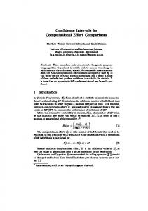
Introduction to Bootstrap Bootstrap draws samples from the Empirical Distribution of data {x1 , x2 , · · · , xn } to replicate statistic T to obtain its sampling distribution. The Empirical Distribution is just a Uniform distribution over {x1 , x2 , · · · , xn }. Therefore Bootstrap is just drawing i.i.d samples from {x1 , x2 , · · · , xn }. The procedure is illustrated by the following graph.

5

Graphical Illustration of Bootstrap Original data

Resampling t

x1(3)

x2(3) x3(3)

x(2) n

T2

x(3) n

T3

x1(B) x2(B) x3(B)

x(B) n

6

.....

x2(2) x3(2)

.....

.....

x1(2)

T1

.....

n

x(1) n

.....

x

. . .n

ing

w Dra

ts poin

x1(1) x2(1) x3(1)

.....

x1 x2 x3

with

.....

men

ace repl

Bootstrap Statistic

TB

Bootstrap Confidence Intervals • Simple Method To obtain the 95% Confidence Interval, the simple method is by taking 2.5% and 97.5% quantiles of the B replication T1 , T1 , · · · , TB as the lower and upper bound respectively. • More Sophisticated Method When the distributions are skewed we need do some adjustment. One method which is proved to be reliable is BCa method( BCa stands for Bias-corrected and accelerated). For the details please refer to DiCiccio, T.J. and Efron B. (1996) [2]

7

Bootstrap Confidence Intervals Given by BCa When the distribution of T is skewed, we instead use the q.low and q.up percentiles of the bootstrap replicates of T to calculate the lower bound and upper bound of the confidence intervals. Formally, for confidence level 95%, z0 + z 0.025 ) q.low = Φ(z0 + 1 − a(z0 + az 0.025 )

(1)

z0 + z 0.975 ) q.up = Φ(z0 + 1 − a(z0 + az 0.975 )

(2)

where z α is the α quantile of standard normal distribution, z0 and a ,namely bias-correction and alleleration, are two parameters to be estimated, by (2.8) and (6.6) in DiCiccio and Efron[2].

8

Confidence Interval of the Average The plot of 10,000 replicates of the sample average:

1000 0

500

Frequency

1500

2000

Histogram of mboot

1.4 e−07

1.6 e−07

1.8 e−07

2.0 e−07

mboot

The 95% confidence interval of the Average calculated by BCa is: 3.196408%

99.32855%

1.399666e − 07 1.871455e − 07 where 3.196408% and 99.32855% is the q.low and q.up given by (1) and (2), similarly for other C.I.s given henceforth. 9

Confidence Interval of 95% Percentile The plot of 10,000 bootstrap replicates of the 95% sample quantile: 800 1000 1200 600 0

200

400

Frequency

Histogram of qboot95

4.4 e−07

4.5 e−07

4.6 e−07

4.7 e−07

qboot95

95% Confidence Interval: 2.381881%

97.41008%

4.400038e − 07 4.626755e − 07

10

Confidence Interval of 99% Percentile The plot of 10,000 bootstrap replicates of the 99% sample quantile:

1000 0

500

Frequency

1500

2000

Histogram of qboot99

1.55e−06

1.60e−06

1.65e−06

1.70e−06

1.75e−06

qboot99

95% Confidence Interval: 2.514489%

97.59096%

1.589317e − 06 1.751419e − 06 11

1.80e−06

Confidence Interval of the probability that the rate exceeds 1.4E-5 The plot:

Frequency

0

500

1000

1500

2000

Histogram of alfa1boot

0.0005

0.0006

0.0007

0.0008

0.0009

0.0010

alfa1boot

95% Confidence Interval: 1.99185%

97.19283%

0.0006151093

0.0009506235 12

0.0011

Confidence Interval of the probability that the rate exceeds 3E-4 The plot:

2000 0

1000

Frequency

3000

Histogram of alfa2boot

0e+00

1e−05

2e−05

3e−05

4e−05

5e−05

6e−05

alfa2boot

95% Confidence Interval: 0.3888835%

93.23166%

0.000000e + 00 2.795951e − 05 13

7e−05

Summary of Results Par.

Estimation

95% Confidence Interval

Average

1.557816e-07

(1.399666e-07,1.871455e-07)

95% Perc.

4.510736e-07

(4.400038e-07,4.626755e-07)

99% Perc.

1.663400e-06

(1.589317e-06,1.751419e-06)

p1

0.0007828664

(0.000615109,0.000950623)

9.319838e-06 (0.00000e+00,2.79595e-05) p2 p1 —Probability that the rate exceeds 1.4e-05 p2 —Probability that the rate exceeds 3.0e-4

14

Reference [1] Davison, A.C. and Hinkley, D.V. (1997) Bootstrap Methods and Their Application, Chapter 5. Cambridge University Press. [2] DiCiccio, T.J. and Efron B. (1996) Bootstrap confidence intervals (with Discussion). Statistical Science, 11, 189-228. [3] Efron, B. (1987) Better bootstrap confidence intervals (with Discussion). Journal of the American Statistical Association, 82, 171-200.

15