Calculation and optimisation model for costs and effects of availability relevant service elements Jürgen Fleischer, Udo Weismann, Stephan Niggeschmidt Institute of Production Science, Universität Karlsruhe, Research University, Germany Abstract The competitiveness of manufacturing companies depends on the availability of their production facilities. The equipment of highly integrated production facilities with robust components and surveillance functionality combined with the right service elements contributes significantly towards securing this availability. In this context there exists an urgent need for research to develop methods allowing the determination of an optimal combination of machine equipment and service elements ensuring defined availability levels. The article describes the development of an integrated approach to determine the complex interdependencies between machine equipment and service levels. Furthermore, the achieved availabilities as well as the resulting costs are displayed. Based on these results, the choice of a machine’s equipment and of service levels shall be harmonised. The main focus of this article is the development of a suitable reliability model combined with the identification of relevant model parameters. Keywords Lifecycle, maintenance, availability
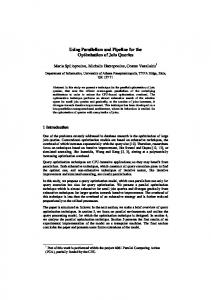
1 INTRODUCTION Operators of production facilities demand information and guarantees regarding Life-Cycle-Cost elements and performance measures as maintenance costs and availability [1]. For the manufacturer this means economic risks but simultaneously bears chances. Particular risks considered in this article are the contractually guaranteed availability levels of machines. On the one hand it is easy to discover these risks. On the other hand it is difficult to calculate them. The worst-case scenario poses the threat of payment obligations throughout the whole contract duration. Selling machines at higher initial costs which are more cost-effective than cheaper alternatives considering their total life-time is a chance of special interest for European manufacturers. Another chance of such contracts consists in collecting experience and operational data during the contract period. First of all this data can be used for machine improvement. Furthermore, a manufacturer can also offer individual services that are specially aligned to the operating behaviour of the machine. In cooperation with the operator these services can lead to the economic optimum. The key figure regarding availability guarantees is the operational availability. Availability is identified as the period of time in which the machine can actually be used for production purposes. Operational availability in that sense takes into account times of technical, administrative, organisational and logistical disruptions of production (Figure 1). In consequence, operational availability is, in essence, determined by the three factors reliability, maintainability of the machine and maintenance readiness of the service organisation [2, 3]. These three aspects in turn have their own influence factors like environment, age or load. For this reason, operational availability relates to all relevant periods that can be directly influenced by the maintenance department (see Figure 1). Since most services have an impact on those time proportions, the service benefit can be expressed by the improvement of the operational availability. Aspects of key figures and dimensions of operational availability regarding reliability [4, 5], maintainability [6, 7] and maintenance readiness [8, 9] are discussed in current literature.
Total Time
Scheduled Busy Time TB Production Time TP
Inherent Availability:
Technical Downtime TF
A( i ) =
Technical Availability:
Unscheduled Busy Time & Interval Time
Downtime for Organisational Maintenance & Downtime Inspection TM TO
MTBF MTBF + MTTR
A(t ) =
Operational Availability: MTBF: Mean Time Between Failure MTTR: Mean Time To Repair
MTBF MTBF + MTTR+ MRDP
A(o) =
MTBF MTBF + MTTR+ MRDP+ MRDA
MRDP: Mean Related Downtime for Preventive Maintenance MRDA: Mean Related Downtime for Administration
Figure 1: Influencing variables regarding operational availability 2 OVERVIEW This article presents first results of a research project funded by the German Research Foundation (DFG). The project aims at the optimisation of the combination of availability-relevant service elements and equipment options that can be offered by a manufacturer. Section 3 outlines the approach and the individual work packages. Section 4 focuses in detail on the data model. The data model establishes the basis for further reliability and availability calculations as well as for later optimization. 3 APPROACH Initially the influence of a machine’s technical equipment, the influence of service elements and the operational environment (maintenance readiness) on operational availability and costs is to be modelled (Figure 2). The attribution of operational data sources to model parameters enables the prognosis of operational availability and maintenance costs of new machine configurations.
675
Afterwards the effect of each service element on operational availability can be evaluated. The first step is the decomposition of malfunction periods (Mean Time To Repair – MTTR) in administrative, logistical, repair-related and technical elements. After that, the effect of individual service elements and equipment attributes on the time elements are analysed (see example in Figure 3). The underlying model identifies specific service elements and provides generic process models. This way, the maintenance processes can be configured for individual organisations and different cooperations for the user. The respective sub-processes are described by:
Figure 2: Critical relation between operational availability and cost according to [10] The underlying approach towards the development of the calculation and optimisation model for costs and effects of availability relevant service elements is divided into five steps: •
Determination of model parameters
•
Identification of interdependencies between equipment attributes and service levels
•
Performance Measurement System for Service Readiness
•
Conception of the calculation tool
•
Validation with real operational data and implementation into tender preparation of machine tool manufacturers
3.1 Determination of model parameters The identification of parameters suitable for setting up the technical reliability model is crucial in this work package. This addresses the issue of sufficient data sources for modelling and later application in prognosis. Additional parameters have to be identified describing the influence of service elements on operational availability. For those parameters in turn data sources have to be found which can later be used for prognosis purposes. The procedure for the calculation of operational availability shall be developed for different types of machine facilities, operational modes and maintenance organisations. Different accuracy requirements and data availabilities of the users have to be taken into account. The defined model parameters should be suitable to represent all possible applications in production technology. The remarks in section 4 focus especially on the development of a reliability and data model for production facilities. 3.2 Identification of interdependencies The next step is the identification of the contribution towards availability of equipment attributes and service elements. At the same time the resource demand has to be detected. First of all the availability contributions of individual service elements as well as their cost structures have to be determined. Later those will be used in the calculation tool to be developed. Furthermore, the impact of alternative and optional machine configurations on availability has to be assessed. The cost structures of machine equipment are usually available and therefore can be used easily. The challenge in this approach is the disentanglement of interdependencies between individual service elements.
676
•
Performance input and output
•
Resource usage
•
Cost factors
•
Procedure times, and
• Quality criteria In the next step potential interdependencies between service and maintenance elements have to be considered. For that purpose, these elements are compared and rated as independent, strengthening or alleviative. For example figure 3 displays independent attributes: The equipment attribute Teleservice (equipment package B) does not influence the effectiveness of the 24h availability of the service. MTBF/MTTF Operation
Downtime
Operation
Downtime
Operation
Net repair time
Setting and warm up
MTTR
Time till Time for technician on site diagnostics
Logistic downtime e.g. for spare part
MTTR with : Tele Service MTTR with Service package II: 24h Service Availability MTTR with equipment package B and Service package II
Figure 3: Influences on MTTR Now the accruement costs of each individual service and equipment element have to be identified. The determined interdependencies and effects of service and equipment elements on availability and costs enable the structuring of those into distinct packages a manufacturer can offer. If these are arranged as in figure 4 for example, it is possible to select them according to resulting costs and availability during tender preparation. Two equipment packages (A, B) are combined with three service packages (I, II, III) resulting in the offers 1 through 6. Offer 5 for example includes the reliability-raising equipment package B in combination with a service package II. This way, the resulting operational availability in percent and the Life-Cycle-Costs can be identified in the portfolio for each possible combination. In this case the Life-CycleCosts are the costs without interest charged to the operator, excluding costs for disruption of production. With the knowledge of his individual costs for disruption of production, the operator can now choose the optimal combination. Since the development of the Life-CycleCosts is known as well, a capital interest rate specified by the operator can easily be calculated and taken into account.
P ROCEEDINGS OF LCE2006
Figure 4: Availability and Life-Cycle-Costs of different equipment and service package configurations 3.3 Performance Measurement System for Service Readiness The model in section 4 describes the reliability and maintainability based influence factors of production facilities. However, to develop an integrated concept for the prognosis of operational availability, it is necessary to determine the influence factors regarding the elimination of production disruptions (Figure 5). The determinants of maintenance readiness are not associated with a single functional unit, but with the production facility or organisation in all. Maintenance readiness itself can be increased by availability-relevant equipment elements like integrated diagnosis functionality, Security-PLC etc. (technical maintenance readiness). Furthermore, this is possible through service organisation (organisational maintenance readiness). Especially the organisational maintenance readiness is composed of manifold factors that can be influenced directly through operational measures. As a consequence the identification of logistical, administrative and organizational parameters influencing significantly maintenance readiness as well as their information sources have to be identified.
Figure 5: Influences on time-related key figures of availability As soon as those determinants are established, the activity times of the maintenance process analysed in section 4 can be aggregated to appropriate time-related key figures (Figure 5). The resulting key figures, like the mean logistic downtime of customer service, go directly into the calculation methodology for reachable operational availability. 3.4 Conception of the calculation tool The application of the approach requires an IT-supported implementation. This is unavoidable due to the large
amount of data needed for statistical validation. Tasks of the scientific implementation are initially the conception of an appropriate calculation tool for tender preparation and the integration of a suitable information basis. The fundamental requirements stem from the use of this tool during the process of tender preparation for complex production systems. In this phase it has to be possible to consider all available information regarding reliability, availability and Life-Cycle-Cost in a fast and easy way. The fundamental data model for the calculation of offers will be described in further detail in section 4. Furthermore, the tool needs to provide interfaces with common software and should be user friendly. To achieve these requirements, which are especially important regarding broad acceptance, the graphical user interface and the software architecture is developed in close collaboration with project managers, IT and sales engineers of several machine manufacturers. Finally, the software is supplemented with suitable methods for the generation of service element and equipment element packages as well as for methods for tender preparation. 3.5 Validation of the approach For verification of practical applicability in the industry, the concept stipulates a validation with example data. Using system data from the industry, the calculation method is tested exemplary for a flexible production system made up of standard machining centers. Thereby, the time and effort needed for the application of the methods will be determined. From the experiences gained in the validation a concept for implementation is to be derived, focussing on the adaptation of the methodology to specific operational conditions. Especially regarding the specification of adequate system boundaries and levels of detail a decision guidance has to be developed taking into account the individual use cases. 4 DATA MODELL AND SOURCES FOR RELIABILITY ANALYSIS AND PROGNOSIS As indicated before, the model considers both the technical reliability of a machine tool as well as the influences on the availability by conducted services. These two input factors are supplemented with their respective demand for resources to enable a modelling of the costs. Structures of the technical specification provide the initial point for a reliability-technological modelling of the examined system. The developed reliability model displays the interdependencies regarding reliability between subcomponents of different aggregation levels in a tree-structure (Figure 6).
Figure 6: Diagram of a system structure model with variants [11] The reliability model of the production systems determines to a large degree the precision for the calculation of the total availability of a system. First of all, the required
13th CIRP I NTERNATIONAL C ONFERENCE ON L IFE C YCLE E NGINEERING
677
accuracy-levels for the description of the examined units and their reliability figures were defined. Finally specific structuring rules were derived. The model is applicable both for single machines and interlinked production systems and ranges to the level of functional units. If desired the user is able to reduce the reliability model to specified subsystems that show critical failure behaviour and need special attention. In this model technical units show constructive and predictable behaviour (reliability and maintenance). Yet they are subject to further influences. Coping with different boundary conditions through various production programs and operational modes of the system, suitable load factors are established (e.g. operating hours, peak forces, maintenance intensity). Depending on these load factors, reliability-related information can be associated with individual functional units of the system. This category consists of different determinants, including for example the Mean Time Between Failure and the fundamental distinction of cases regarding failure modes and effects. Reliability of a machine is characterised respectively by its failure frequency and failure behaviour. This can be described by the MTTF (Mean Time To Failure) value or, if it is a maintainable unit, by its MTBF (Mean Time Between Failure) value [12]. However, this distinction is not applied universally in literature. Usually the term MTBF is used instead of MTTF for both maintainable and non-maintainable machines. Since a distinction does not bring additional benefit to the given approach, only the term MTBF will be used in the following. This term regards the total runtime of a machine in relation to its failure frequency. However a MTBF value on machine level is not enough to estimate accurately the extent of maintenance. This is due to the fact that maintenance efforts (MTTR, spare part costs, personnel qualification etc.) differ between individual failures. In consequence, the calculation of the MTBF value at assembly group and component level is carried out. To calculate the operational availability, losses of time due to maintenance during planned machine busy time have to be recorded. These losses of time are caused by machine failures. Their duration depends on maintainability, reaction time and service performance of the maintenance department (Figure 7).
Disaggregating the MTTR (downtime interval) leads to the individual time units (Ξ1,… Ξn). Each characteristic time unit correspond to individual phases during the maintenance process. Basically these phases do not have a particular order. Thus, the diagnosis of the problem for example can take place prior to the error message by the customer, just after the error message by means of teleservice or local customer service. Crucial to the disaggregation is that each activity and idle time can be distinctly associated with a single phase and that either the manufacturer’s service or the customer is responsible. If required, the main phases should be partitioned into subordinate activities [13]. The six exemplary time units in figure 7 include: •
Administrative stand by time (Ξ1 to Ξ3) defined as latency caused by communication and assignment processes in addition to non-reachability issues. Since failure diagnosis is a cooperative process between a customer and a manufacturer it is part of this category.
•
Logistical stand by time (Ξ4a to Ξ4d) for the preparation and provision of all necessary resources for repair. They do not occur in every service case.
Component-dependent downtimes (Ξ5 and Ξ6) due to technological reasons. The maintenance process is not completed with the return to operation. In addition to the specific downtime units time and effort of the customer’s service for documentation, travelling etc. accrues. Even though these factors are not relevant for the calculation of availability, they should be considered at this stage as essential for the determination of resource demand later on. Generally speaking, incoming information for reliability and availability calculations is afflicted with uncertainties. Due to the fact that units from different production technologies and operational conditions are aggregated, some failure causes and their interdependencies remain unconsidered and control samples are coincidental. Thus an essential success factor for availability analysis is the consistent gathering and use of information about the machine’s operational behaviour [14, 15]. Hence all available data sources both on the operator’s and on the manufacturer’s side should be reviewed in regard to the appropriation for the reliability analysis [16]. The following sources exist on the operator’s side: •
•
•
Figure 7: Characteristic downtime units for mathematic modelling
678
Operational data: Field data of existing machine populations gathered under real operating conditions is fundamental for any reliability analysis and prognosis. Oftentimes this data is recorded under uncontrolled conditions or else the data is not representative (for example datasets provided by the operator to strengthen a warranty claim). This is why the selection of objects is of great importance [17]. Through constructive improvements within a type series, the examined units as a whole can become inhomogeneous. Examining at a component level can exclude those effects. Maintenance data: if planned machine busy times are known, records and statistics of the operator’s maintenance services theoretically enable the calculation of MTBF and MTTR values. In practical experience, however, the quality of data is mostly not ideal. Failures for example are not associated with the respective component, but rather with the machine or even the production system. This prohibits the reliability analysis on component level at a later point in time.
P ROCEEDINGS OF LCE2006
On the manufacturer’s side the following data sources are of interest: •
•
•
•
•
•
Customer service data: The customer service documents the reliability-relevant failures commissioned by a customer for repair or warranty claims. In common business models this is primarily the case during the warranty period, wherefore later records are limited. Spare part demand and sales: This data source is of special interest if only little maintenance and service data is available. Failures within component level, oftentimes even related to individual machines, can be concluded from the booking of spare part sales. For internal analysis at the operator, booking records of internal spare part storages can be used to improve the quality of maintenance data. Using the material numbers of spare parts wrong allocations can be corrected. However, this data source is usually incomplete as well. Spare parts that are bought for storage purposes interfere with the calculation of failure frequencies on assembly group level just like spare parts that were bought directly from the component supplier instead of the machine manufacturer. Test and simulation data: Test and simulation data often exists on the manufacturer’s side, especially on component level, since this data is needed for the development process. The advantage of tests is their carefully controlled experimental conditions that allow, particularly concerning loads, the examination and determination of the influence of individual factors. Reliability specifications by component suppliers and general information on common components, like [18, 19] are also classified as test data. Dimensioning calculations: The classical approach towards reliability prognosis is component dimensioning following norms and component supplier specifications. Particularly standard components allow the calculation of their lifetime and standard deviation with high statistical confidence. For this, however, precise knowledge of loads and operating conditions is required. Yet, concerning machines made to specifications like special machines or universal machine tools this knowledge does not exist. Expert estimation, FMEA, FTA: Expert estimation is used as substitute or to enrich existing data. Expert estimation can also be used to judge the quality of real data. The degree of subjectiveness has to be taken into account regarding the choice of an estimation method. The essential methods of determining reliability-relevant data by expert estimation are the FMEA (Failure Mode and Effect Analysis) and the FTA (Fault Tree Analysis). They identify all possible failure causes and provide an estimation of the probability of their occurrence. Within the scope of this approach a FMEA is carried out focussing on errors occurring during operation. The causes are then linked with the probabilities by boundary conditions. For example causes related to wear are associated with higher probability with increasing runtime of the machine. In doing so, the probability of failure is quantified and expressed in MTBF values [20]. Value analysis: Functional structure and costs from value analysis can be used to structure and complete the data model in the introduced approach. The determination of functional costs and value as a result of this analysis has to be executed with respect
to the lifecycle. Therefore costs considerations on a functional level have to be supplemented by costs for servicing and maintenance. The following figure 8 summarizes all relevant available data sources for reliability and availability calculations:
Figure 8: Data sources As mentioned above problems arise during the collection of operational and customer service data that limit the analytic possibilities. Predominantly the small number of recorded failures easily leads to inaccuracies and incorrect interpretation [21]. If data collection simply focuses on failures per time unit, implicit assumptions are made that can possibly cause biased prognoses. These assumptions include constant failure rates, even though in most cases serial correlations and trends are encountered [22]. Furthermore, independent failures, homogeneous production systems and operating conditions are often presumed. Considering these deficits data collection bears the following requirements in this approach: •
Careful identification of the examination object and its regular operating conditions • Precise chronological recording of failure and repair times • Recording of actual runtimes and loads as well as preventive maintenance measures and repair qualities As collection of data enabling reliability analysis has a significant effort, its benefits have to be evaluated for the individual case. The goal has to be the extensive utilization of existing informational systems as well as the continuous collection of data throughout the whole lifecycle of the examination objects. Methods of resolution for this purpose are presented in [23]. Furthermore, it has to be noted that datasets coincile in certain points. These intersections contain information that exists both on the operator’s and on the manufacturer’s side. This is the case if, for example, an operator uses a spare part supplied by a manufacturer. In the context of an analysis, the challenge is to identify those intersections to avoid a double consideration, which would bias the results. Finally, the generation of high quality data can only be achieved by means of close cooperation of all parties. 5 SUMMARY The introduced approach was developed in a research project funded by the German Research Foundation (DFG). It visualises the influence of additional services provided by a machine manufacturer through the construct of availability contributions. These availability contributions of service elements and equipment attributes cause the shortening of certain time units in the
13th CIRP I NTERNATIONAL C ONFERENCE ON L IFE C YCLE E NGINEERING
679
repair process. A method determining these contributions was introduced. The focus of this publication is on the underlying reliability and data model as a first result of the research project. The method calculates the expected availability level, the costs for securing the availability and the costs of nonavailability for each combination of equipment and service elements and operating conditions. For this purpose it extends the common structure models of production systems by the representation of component dependent availability attributes, which are described probabilistically. For the determination of the maintenance timings, all associated processes are classified so that both the number of participants and influence factors for each subprocess are manageable. A fundamental prognosis step is then to identify the effects of service elements on the subprocesses. This step uses a procedure to reduce complexity in terms of acceptable combinations of service elements that can be adapted to the individual use case. That way the expected marginal utility of a more accurate prognosis can be weighted against the additional analytical effort. A software prototype will carry out the necessary calculation steps and makes the method usable in practical application. REFERENCES [1] Stauch, V., 2004, Total Cost of Ownership (TCO) bei Daimler Chrysler – ein Beitrag zur wirtschaftlichen Produktionseinrichtung, Proceedings of the 2004 wbk Autumnal Conference Life-Cycle-Performance, ISSN 1618-1484, Vol. 11, Institute of Production Science, Karlsruhe. [2] Kumar, U.D., Knezevic, J., 1998, Supportability – critical factor on system’s operational availability, International Journal of Quality & Reliability Management. [3] Verein Deutscher Ingenieure, 1986, VDI-Richtlinie 4004, Blatt 4, Zuverlässigkeitskenngrößen – Verfügbarkeitskenngrößen, Beuth, Berlin. [4] Birolini, A., 2004, Reliability Engineering – Theory and Practice, 4th ed., Berlin, Springer. [5] Blischke, W.R., Murthy, D.N.P., 2000, Reliability – Modeling, Prediction, and Optimization, Wiley, New York. [6] Blanchard, B.S., Verma, D., Peterson, E.L., 1995, Maintainability, Wiley, New York. [7] Wani, M.F., Gandhi, O.P., 1999, Development of maintainability index for mechanical systems, Reliability Engineering and System Safety, 65:259270. [8] Goffin, K., 2000, Design for Supportability: Essential Component of New Product Development, Research-Technology Management, 43/2:40-47. [9] Markeset, T., Kumar, U., 2003, Design and development of product support and maintenance concepts for industrial systems, Journal of Quality in Maintenance Engineering, 9/4:376-392. [10] Fleischer, J., Nesges, D., 2005, Lifecycle CostModelling for Machinery with Specified Availability Levels, CIRP Reconfigurable Manufacturing Systems, Ann Arbor.
680
[11] Fleischer, J., Nesges, D., 2005, Identifying Availability Contribution of Lifecycle-adapted Services, CIRP Life Cycle Engineering, Grenoble. [12] DIN EN 61703, 2002, Mathematical expressions for reliability, availability, maintainability and maintenance support terms; German version, Beuth, Berlin. [13] Seufzer, A., 2000, Durchgängige Unterstützung von Instandhaltungsprozessen, Fortschr.-Ber. VDI-Reihe 2, Nr. 539, VDI-Verlag, Düsseldorf. [14] Köhrmann, C.; Wiendahl, H.-P., 1998, International Strategies Used for Availability Optimisation of Assembly Systems, International Journal of Advanced Manufacturing Technology. [15] Deutsche Gesellschaft für Qualität e.V., 2002, Zuverlässigkeitsmanagement – Einführung in das Management von Zuverlässigkeitsprogrammen, Beuth, Berlin. [16] DIN EN 60300-3-2, 2005, Dependability management – Application guide – Collection of dependability data from field; German version, Beuth, Berlin. [17] Loss, H.-J., 1996, Optimierung von Instandhaltungsstrategien durch rechnerunterstützte Betriebsdatenanalyse und -verarbeitung, Fortschrittsberichte VDI, VDI Verlag, Düsseldorf. [18] Department of Defense, 1995: MIL-HDBK 217 F, Reliability Prediction of Electronic Equipment, Washington D.C.. [19] Naval Surface Warfare Center (Hrsg.): NSWC98/LE1, Handbook of Reliability Prediction Procedures for Mechanical Equipment, Naval Surface Warfare Center, Carderock Division, West Bethesda 1998. [20] DIN 25448, 1990, Ausfalleffektanalyse (FehlerMöglichkeits- und Einfluß-Analyse), Beuth, Berlin. [21] Márquez, A. C.; Herguedas, A. S., 2004, Learning about failure root causes through maintenance records analysis, Journal of Quality in Maintenance Engineering 10. [22] Walls, L. A.; Bendell, A., 1986, The Structure and Exploration of Reliability Field Data: What to Look For and How to Analyse It, Reliability Engineering 15. [23] Niestadtkötter, J., 2000, Methodik zur ganzheitlichen Dokumentenund Datenstrukturierung im Lebenslauf komplexer Werkzeugmaschinen, JostJetter-Verlag, Heimsheim.
CONTACT Jürgen Fleischer Institute of Production Science, Universität Karlsruhe, Kaiserstr. 12, 76128 Karlsruhe, Germany,
[email protected]
P ROCEEDINGS OF LCE2006