Unified approach for optimisation of single-user and multi ... - CiteSeerX

Unified approach for optimisation of single-user and multi-user multiple-input multiple-output wireless systems

von Diplom-Ingenieur Eduard Axel Jorswieck aus Berlin

von der Fakult¨at IV - Elektrotechnik und Informatik der Technischen Universit¨at Berlin zur Erlangung des akademischen Grades

Doktor der Ingenieurwissenschaften - Dr.-Ing. -

genehmigte Dissertation

Promotionsausschuss Vorsitzender: Prof. Dr. Gerhard M¨onich Berichter: Prof. Dr. Dr. Holger Boche Berichter: Prof. Dr. Bj¨orn Ottersten (KTH Stockholm) Tag der wissenschaftlichen Aussprache: 13. September 2004

Berlin 2004 D 83

Zusammenfassung Mehrantennensysteme werden in zuk¨ unftigen Mobilfunksystemen der dritten und vierten Generation eingesetzt werden, um die spektrale Effizienz, die Zuverl¨ assigkeit ¨ und die Qualit¨at der drahtlosen Ubertragung zu verbessern. In der Theorie wurde bewiesen, dass die Kanalkapazit¨ at dieser Mehrantennensysteme linear steigt mit der Anzahl der verwendeten Sende- und Empfangsantennen. Eine andere wichtige Kenngr¨ oße neben der Kanalkapazit¨at ist der mittlere quadratische Fehler, wenn der optimale lineare Empf¨ anger eingesetzt wird. Beide Kenngr¨ oßen variieren mit den Eigenschaften des Mehrantennen-Kanals und des betrachteten Systems, z.Bsp. mit der Art der Kanalinformation am Sender und Empf¨ anger. Sogar partielle Kanalinformation am Sender erh¨ oht die Leistungsf¨ ahigkeit des Mehrantennensystems betr¨ achtlich. In dieser Arbeit werden die Eigenschaften von Mehrantennensystemen mit einem oder mit mehreren Benutzern in einem zellularen Kontext analysiert und neue optimale Sendestrategien entworfen, die die statistischen Eigenschaften des r¨ aumlichen Kanals und die Art der Kanalinformation am Sender ber¨ ucksichtigen. Im Szenario mit einem Teilnehmer wird die mittlere Leistungsf¨ ahigkeit des Mehrantennensystems unter dem Einfluss von einem r¨ aumlich korreliertem Schwundkanal und mit verschiedenen Arten von Kanalinformationen am Sender und mit perfekter Kanalkenntnis am Empf¨ anger analysiert. Zuerst wird ein mathematisches Maß f¨ ur die r¨ aumliche Korrelation basierend auf der Majorisierungstheorie definiert. Dadurch wird es m¨ oglich, die mittlere Performanz als Funktion der sende- und empfangsseitigen Korrelation im Kontext von Schur-konvexen und Schur-konkaven Funktionen zu beschreiben. Ausserdem stellt man fest, dass die Performanz-Maße zu einer allgemeinen Klasse von Funktionen geh¨ oren, die als Spur einer matrixmonotonen Funktion darstellbar sind. Wir verwenden L¨ owners Darstellung von operator-monotonen Funktionen, um auf einer abstrakten Ebene die optimalen Sendestrategien und den Einfluss der Korrelation auf die Performanz zu charakterisieren. Die optimale Sendestrategie ohne Kanalkenntnis am Sender ist eine Leistungsgleichverteilung in alle Richtungen. Dieses Ergebnis wird f¨ ur r¨ aumlich korrelierte Kan¨ ale bewiesen, indem die robusteste Sendestragie gegen die schlechteste Korrelation berechnet wird. Die mittlere Performanz ohne Kanalinformation am Sender ist eine Schur-konkave Funktione bez¨ uglich Korrelation am Sender oder Empf¨ anger. Desweiteren, wird die optimale Sendestrategie f¨ ur den Fall hergeleitet, in dem der Sender die Langzeitstatistik des Kanals kennt. Ein iterativer Algorithmus l¨ ost das Problem der optimalen Leistungsverteilung. Die sogenannte Beamforming-Region ist der SNR Bereich, in dem ein einziger r¨ aumlicher Datenstrom die maximale mittlere Leistung erreicht. Dieser SNR Bereich ist relevant, da hier eine sehr einfache Emf¨ angerstruktur und eine gut verstandene Kanalkodierung eingesetzt werden k¨ onnen. Schließlich leiten wir die generalisierte Waterfilling L¨ osung als optimale Sendestratgie f¨ ur perfekte Kanalkenntnis am Sender und Empf¨ anger her und charakterisiern die Eigenschaften dieses Verfahrens. In einem zellularen Mobilfunksystem greifen mehrere Teilnehmer zur gleichen Zeit auf derselben Frequenz auf eine gemeinsame Basisstation zu oder eine Basisstation sendet gleichzeitig Daten f¨ ur mehrere Teilnehmer. Die Interzell- und Intrazellinterferenz in einem solchen System erzeugt r¨ aumlich gef¨ arbtes Rauschen auf einer einzelnen Mobilfunkstrecke. Daher kann als erster Ansatz ein Mehrantennensys-

I

tem mit einem Teilnehmer und gef¨ arbtem Rauschen betrachtet werden. Wir leiten die Performanz unter dem schlechtesten m¨ oglichen Rauschen und unter verschiedenen Annahmen bez¨ uglich des Rauschens her, um Einsichten in die erreichbare Performanz des Mehrantennensystems im zellularen Kontext mit Inter- und Intrazellinterferenz zu erhalten. Durch bestimmte Rauschf¨ arbung kann sowohl die Kanalkenntnis als auch die Kooperationsf¨ ahigkeit an den Sendeantennen verloren gehen. Der n¨ achste Schritt besteht darin, die Sendestrategien aller Teilnehmer einer Zelle zu ber¨ ucksichtigen. Im letzten Abschnitt der Arbeit wird die augenblickliche Summen-Performanz des Mehrantennen Mehrfachzugriffskanals und des Mehrantennen Broadcast-Kanals unter individuellen oder Summenleistungsbeschr¨ankungen maximiert. Als Summen-Performanz wird entweder die Summenkapazit¨at mit sukzessiver Interferenz-ausl¨ oschung im Uplink oder mit Costa-Vorkodierung im Downlink, sowie der normierte mittelere quadratische Summenfehler eingesetzt, falls ein Mehrbenutzer-MMSE Empf¨ anger verwendet wird. Die gemeinsame Kovarianzmatrixoptimierung kann unter Verwendung der Karush-Kuhn-Tucker Optimalit¨ atsbedingungen in eine abwechselnde Leistungsoptimierung und normierte Kovarianzmatrixoptimierung zerlegt werden. Letztere wiederum zerf¨ allt in eine Art modifizierte Einbenutzer Kovarianzmatrixoptimierung mit gef¨ arbtem Rauschen. Die konkrete Struktur dieser Einbenutzer Optimierung h¨ angt von der konkreten PerformanzMetrik ab. Der vorschlagene iterative Algorithmus l¨ ost das Summen-Performanz Optimierungsproblem auf effiziente Weise.

II

Abstract Multiple-input multiple-output (MIMO) systems will be applied in wireless communications in order to increase the performance, spectral efficiency, and reliability. Theoretically, the channel capacity of those systems grows linearly with the number of transmit and receive antennas. An important performance metric beneath capacity is the normalised mean square error (MSE) under the assumption of optimal linear reception. Clearly, both performance measures depend on the properties of the MIMO channel as well as on the considered system approach, e.g. on the type of channel state information which is available at the transmitter. It has been shown that even partial CSI at the transmitter can increase the performance. In this thesis, we analyse the performance and design optimal transmit strategies of single- and multiuser MIMO systems with respect to the statistical properties of the fading channel and under different types of CSI at the transmit side. In the single-user scenario, we study the average performance of the system under spatial correlated fading and with different types of CSI at the transmitter and with perfect CSI at the receiver. First, we introduce a measure of correlation which is based on Majorization. As a result, the average performance is analysed as a function of correlation in the context of Schur-convexity and Schur-concavity. Furthermore, we observe that the performance metrics belong to a general class of functions which are the trace of a matrix-monotone function. We use L¨ owner’s representation of operator monotone functions in order to derive the optimum transmission strategies and to characterise the impact of correlation on the average performance. The optimal transmit strategy without CSI at transmitter is equal power allocation. We prove this result for spatial correlated channels by analysing the most robust transmit strategy under worst case correlation. The average performance without CSI is a Schur-concave function with respect to transmit and receive correlation. In addition to this, we derive the optimal transmission strategy with long-term statistics knowledge at the transmitter and propose an iterative algorithm. The beamforming-range is the SNR range in which only one data stream spatially multiplexed achieves the maximum average performance. This range is important, because of its simple receiver structure and well known channel coding. Finally, we derive the generalised water-filling transmit strategy for perfect CSI and characterise its properties. If the single-user MIMO link is placed into a cellular system in which multiple users at the same time on the same frequency access one common base station or in which one base station transmits to multiple users, the interference colours the noise. This means, we can continue to study a single-user link now with coloured noise as a first approach. In order to gain insights into the performance under interference conditions, we derive the worst case noise performance for three different noise scenarios. We show that the cooperation and the CSI at the transmitter get lost if some type of worst case noise is applied. If all transmit strategies of all participating users are incooperated into the analysis, we arrive at the multi-user MIMO system. Finally, we maximise the instantaneous sum performance of MIMO multiple access channels (MAC) or broadcast channels (BC) under individual or sum power constraints. The sum performance is either the sum capacity if SIC is applied in the uplink or if Costa Precoding is applied in the downlink, or the normalised sum MSE if a

III

multiuser MMSE receiver is applied at the base. Using the Karush-Kuhn-Tucker optimality conditions, we show that the mutual covariance matrix optimisation can be decomposed into power allocation and covariance matrix optimisation under individual power constraints, which can be decomposed into a kind of modified single-user covariance matrix optimisation treating the other users as noise. The concrete structure of the single-user program depends on the performance metric. The proposed algorithms efficiently solve the multi-user MIMO sum performance optimisation problem.

IV

Acknowledgements During my PhD studies, I had the opportunity to meet many interesting and extraordinary individuals. First of all, I thank my advisor Professor Holger Boche for taking his time to guide and support me throughout the three years. He always made it possible to share and discuss ideas and problems. I am very fortunate to have learned information theory and related mathematics from such a great teacher. His enthusiasm, knowledge, energy, and visions have motivated me to a great extent and will have a lasting effect. I thank Professor Bj¨ orn Ottersten for serving as second referee and reader of this dissertation. I want to thank Aydin Sezgin for sharing ideas and room with me during our PhD studies. The comments of Oliver Henkel improved the representation of this thesis. Many thanks go to my project leader Clemens von Helmolt as well as to Volker Jungnickel who have proposed many interesting problems which concerned implementation and realization aspects of multiple-antenna systems. My gratitude extends to Thomas Haustein, Martin Schubert, Gerhard Wunder, Slawomir Sta´ nczak, Tobias Oechtering, Marcin Wiczanowski, Volker Pohl, and Peter Jung for collaborating and co-authoring papers with me. I would like to thank all colleagues at the Heinrich-Hertz-Institut and the Technical University of Berlin for stimulating discussions and additional support.

V

VI

Contents

1 Introduction 1.1 Motivation . . . . . . . . . . . . . . . . . . . . . . . . . . . . . . . . 1.2 Notation . . . . . . . . . . . . . . . . . . . . . . . . . . . . . . . . . . 1.3 Performance metrics and preliminaries . . . . . . . . . . . . . . . . . 1.3.1 Single-user systems: Mutual information and related average performance metrics . . . . . . . . . . . . . . . . . . . . . . . 1.3.2 Multiuser systems: Sum performance metrics . . . . . . . . . 1.4 Outline of the thesis . . . . . . . . . . . . . . . . . . . . . . . . . . .

1 1 2 2

2 Single-user multiple-antenna optimisation 2.1 Related work . . . . . . . . . . . . . . . . . . . . . . . . . . . . . . . 2.2 Channel model and basic definitions . . . . . . . . . . . . . . . . . . 2.2.1 Channel model . . . . . . . . . . . . . . . . . . . . . . . . . . 2.2.2 A mathematical measure of correlation . . . . . . . . . . . . . 2.3 Average performance metrics . . . . . . . . . . . . . . . . . . . . . . 2.3.1 Properties of the inner matrix-valued performance function: Matrix-concavity . . . . . . . . . . . . . . . . . . . . . . . . . 2.3.2 Optimum transmission strategies . . . . . . . . . . . . . . . . 2.3.3 Impact of correlation on the average performance in MIMO channels . . . . . . . . . . . . . . . . . . . . . . . . . . . . . . 2.3.4 Impact of correlation on the average performance in MISO systems . . . . . . . . . . . . . . . . . . . . . . . . . . . . . . 2.3.5 Comparison of average performance results between MIMO and MISO systems . . . . . . . . . . . . . . . . . . . . . . . . 2.3.6 Numerical results and discussion . . . . . . . . . . . . . . . . 2.4 Proofs . . . . . . . . . . . . . . . . . . . . . . . . . . . . . . . . . . .

13 13 15 15 17 20

3 Multi-user multiple-antenna optimisation 3.1 Introduction . . . . . . . . . . . . . . . . . . . . . . . . . . . . . . . . 3.2 Worst Case Noise Analysis in Multiuser MIMO Systems . . . . . . . 3.2.1 Motivation and related results . . . . . . . . . . . . . . . . . 3.2.2 Noise scenarios . . . . . . . . . . . . . . . . . . . . . . . . . . 3.2.3 Applications . . . . . . . . . . . . . . . . . . . . . . . . . . . 3.2.4 Preliminaries . . . . . . . . . . . . . . . . . . . . . . . . . . . 3.2.5 Worst case noise with trace constraint . . . . . . . . . . . . . 3.2.6 Worst case noise directions . . . . . . . . . . . . . . . . . . . 3.2.7 Worst case coloured noise . . . . . . . . . . . . . . . . . . . . 3.2.8 Interpretation and discussion of worst case noise analysis . . 3.2.9 Comparison of worst case noise capacities . . . . . . . . . . . 3.3 Sum Performance Analysis of Multiuser MIMO Systems . . . . . . . 3.3.1 Signal model and sum performance measures . . . . . . . . . 3.3.2 Problem statements: Sum performance optimisation under different power constraints . . . . . . . . . . . . . . . . . . . . 3.3.3 Optimisation of sum performance . . . . . . . . . . . . . . . . 3.3.4 Properties of optimal transmit strategy . . . . . . . . . . . . 3.3.5 Discussion of sum performance optimisation algorithm . . . .

65 65 67 67 68 69 72 74 75 76 79 79 80 80

2 5 8

23 25 34 40 44 46 51

84 85 91 92

VII

Contents 3.4

Proofs . . . . . . . . . . . . . . . . . . . . . . . . . . . . . . . . . . .

4 Conclusions and future research 4.1 Conclusions . . . . . . . . . . . . . . . . . . . . . . . . . . . . . 4.2 Future research . . . . . . . . . . . . . . . . . . . . . . . . . . . 4.2.1 Outage capacity and delay limited capacity . . . . . . . 4.2.2 Individual QoS requirements and network optimisation . 4.2.3 Extension to multi-carrier communications . . . . . . .

. . . . .

. . . . .

. . . . .

92 103 103 104 104 104 105

Publication List

106

References

110

VIII

List of Figures 1.1

Block flat-fading MIMO system. . . . . . . . . . . . . . . . . . . . .

3

2.1 2.2 2.3

Signal processing structure for the MIMO system. . . . . . . . . . . Example correlation matrix eigenvalue distribution. . . . . . . . . . . Capacity as a function of correlation for MISO 2 × 1 system with different levels of CSI . . . . . . . . . . . . . . . . . . . . . . . . . . . SNR range of beamforming over correlation λT1 . . . . . . . . . . . . . Open-loop average mutual information, closed-loop and covariance feedback ergodic MIMO channel capacity over transmit correlation with uncorrelated receive antennas. . . . . . . . . . . . . . . . . . . . Open-loop average mutual information, closed-loop and covariance feedback ergodic MIMO channel capacities over receive correlation with correlated transmit antennas λT = [0.6; 0.4]. . . . . . . . . . . .

15 20

2.4 2.5

2.6

3.1 3.2 3.3

3.4 3.5 3.6 3.7 3.8

Cellular MIMO multiuser uplink. . . . . . . . . . . . . . . . . . . . . Cellular MIMO multiuser downlink . . . . . . . . . . . . . . . . . . . Worst Case Noise with Trace Constraint: Vector MIMO channel ΦI with perfect CSI and worst case noise and corresponding vector MIMO channel without CSI and white noise (Theorem 8). . . . . . . Worst Case Noise Directions: Vector MIMO channel ΦII and corresponding diagonalised orthogonal channels ΦD II . . . . . . . . . . . . Worst Case Coloured Noise: Vector MIMO channel ΦIII and corresponding SIMO MAC ΦD III . . . . . . . . . . . . . . . . . . . . . . . . MIMO MAC system. . . . . . . . . . . . . . . . . . . . . . . . . . . . MIMO BC system. . . . . . . . . . . . . . . . . . . . . . . . . . . . . Sum Performance Optimisation Algorithm . . . . . . . . . . . . . . .

43 47

48

50 70 71

74 76 77 81 83 93

IX

List of Figures

X

List of Tables 2.1

2.2

2.3

2.4

Optimal transmission schemes in MIMO and MISO systems with respect to the average performance with different types of CSI at the transmitter and perfect CSI at the receiver. . . . . . . . . . . . . . . Impact of transmit correlation in MISO systems on the average performance with different types of CSI at the transmitter and perfect CSI at the receiver. . . . . . . . . . . . . . . . . . . . . . . . . . . . . Impact of transmit correlation in MIMO systems on the average mutual information and on the ergodic capacity with different types of CSI at the transmitter and perfect CSI at the receiver. . . . . . . . . Impact of receive correlation in MIMO systems on the average performance with different types of CSI at the transmitter and perfect CSI at the receiver. . . . . . . . . . . . . . . . . . . . . . . . . . . . .

45

46

46

46

XI

Abbreviations and nomenclature

αk (p) Optimality condition coefficients, see equation (2.41), page 33 R∞ Ei(a, b) Exponential integral Ei(a, b) = 1 exp(−κb)κ−a dκ, page 32 ˆk w

Column of white random matrix W with transmit correlation, see equation (2.24), page 26

CN(m, c) Complex normal distribution with mean m and covariance c, page 5 I

Set of active directions or users, page 111

L

Lagrangian function, page 105

λ(X) Eigenvalues of arbitrary Hermitian matrix X, page 84 λR λ

T

ΛZ

Vector of eigenvalues of receive correlation matrix, page 19 Vector of eigenvalues of transmit correlation matrix, page 19 Diagonal matrix with eigenvalues of noise covariance matrix, page 84

λTcc , λR cc Vector of eigenvalues of fully correlated transmit and receive correlation matrix, page 40 λTnc , λR nc Vector of eigenvalues of completely uncorrelated receive and transmit correlation matrix, page 40 H

Flat-fading MIMO channel matrix, page 3

Hk

Channel matrix of user k, page 104

hij

Entry in the i-th column and j-th row of the channel matrix H, page 19

n

Noise vector, page 4

Q

Transmit covariance matrix, page 5

Qk

Transmit covariance matrix of user k, page 104

RR

Receive correlation matrix, page 18

RT

Transmit correlation matrix, page 18

W

Random matrix with ’white’ iid zero-mean complex Gaussian entries, page 18

x

Transmitted signal vector, page 4

y

Received signal vector, page 4

Z

Noise covariance matrix, page 84

Φ

(Average) performance metric, page 24

φ

Inner matrix-monotone performance function, page 24

ρ

SNR: ratio of transmit power to noise power at receiver, page 5

2 σN

Noise power, page 84

˜k w

Column of white random matrix W with receive correlation, see equation (2.22), page 26

C

Average channel capacity, page 6

c F

Instantaneous channel capacity, page 6 [1]

(x) First derivative of matrix-monotone function F , first divided difference at x , see equation (2.31), page 28

h(x)

Entropy of random variable x, page 3

I(a; b) Mutual information between a and b, page 4 K

Number of mobile users, page 7

M SE Average normalized MSE, page 6 mse

Instantaneous normalized MSE, page 6

M SEk Achievable normalised MSE of user k, page 8 nR

Number of receive antennas, page 3

nT

Number of transmit antennas, page 3

P

Transmit power constraint, page 5

pk

Individual power constraint of user k or direction k, page 18

Rk

Achievable transmission rate of user k, page 8

ARQ

Automatic Repeat reQuest, page 1

BC

Broadcast Channel, page 2

CSI

Channel State Information, page 2

DSL

Digital Subscriber Line, page 125

DSM

Dynamic Spectrum Management, page 125

iid

Identically Independent Distributed, page 13

LOS

Line Of Sight, page 13

MAC Multiple Access Channell, page 2 MAP Maximum A-Posteriori, page 6 MIMO Multiple Input Multiple Output, page 1 MISO Multiple Input Single Output, page 1 ML

Maximum Likelihood, page 6

MMSE Minimum Mean Square Error, page 6 OFDM Orthogonal Frequency Division Multiplexing, page 128 pdf

Probability Density Function, page 13

QoS

Quality of Service, page 13

SIC

Successive Interference Cancellation, page 2

SIMO Single Input Multiple Output, page 1 SNR

Signal to Noise Ratio, page 1

TDMA Time Division Multiple Access, page 2 WLAN Wireless Local Area Network, page 1

1 Introduction 1.1 Motivation In mobile communication networks, the properties of the underlying physical channel have great impact on the performance and reliability of the system. The fading channel varies in time, frequency, and space. From a traditional point of view, these fluctuations are the limiting factor of wireless communication. From an information theoretic point of view, these fluctuations can be exploited. They provide the possibility to communicate even more reliable and secure. Recently, the spatial dimension was found to increase the performance and spectral efficiency of a wireless system by simply adding more transmit and receive antennas [FG98, Tel99] under idealistic assumptions. Since those papers were published, multiple antenna techniques have developed to the most active area in research in wireless communications. As a result, the industry and standardisation bodies considered multiple-input multiple-output (MIMO) systems as a promising approach in order to obtain reliable high transmission rates which are required to satisfy the users needs. It is certain that the technology needs to deliver higher data rates to the consumer at a lower cost per data bit. One technology that has been proposed is the use of multiple antennas at both the cellular side and handsets. Other important considered techniques beneath MIMO are adaptive modulation and coding, hybrid ARQ, and fast cell selection [3gp01, 3gp02]. Dual-antenna diversity is already used on WLAN PC cards, access points, and personal digital cellular handsets in Japan. However, the antenna diversity is used only by antenna selection. Most major antenna infrastructure manufacturers offer smart antenna systems. Theoretically, multiple antennas have been shown to enable major increase in the data capacity, peak data rate, performance, and reliability. However, the actual achievable performance depends on the properties of the radio signal propagation environment. Furthermore, the performance of MIMO systems depend on the type and amount of channel state information (CSI) at the receiver and transmitter side. In contrast to the spectral dimension which comes without the cost of interference between orthogonal subcarriers, the signals in space are multiplexed and interfere with each other. By using sophisticated transmit strategies with perfect or partial CSI at the transmitter, it is possible to fully exploit the spatial dimension. Interestingly, depending on the type of CSI, the properties of the channel have different impact on the optimal transmit algorithms and on the achievable performance. Because of the wide range of possible MIMO techniques, it is important to better understand the theoretical limits of MIMO channels and the right techniques which are able to achieve these limits. One important property of MIMO channels is the correlation at the transmit and receive antenna array [GBGP02, CTK02]. This thesis provides an analysis of the maximal achievable reliable transmission rate of single-user and multi-user MIMO systems. The first half is devoted to single-user MIMO systems and their average performance under different types of CSI and under transmit and receive correlation. The second half analyses multi-user MIMO systems in terms of worst case noise analysis and sum performance optimisation under individual and sum power constraints.

1

1 Introduction

1.2 Notation Vectors are denoted in bold letters x. Matrices are written in bold capital letters H. Transpose is [·]T , the conjugate transpose is [·]H . The matrix (pseudo) Pninverse is denoted by [·]−1 . tr(A) denotes the trace of the matrix A, i.e. tr(A) = k=1 Ak,k . λi (A) is the ith eigenvalue of the matrix A. λmax (A) is the largest eigenvalue of n the matrix A. R(x) denotes the real part of the complex variable x. C + denotes the P n set of positive semidefinite matrices. ||a|| is the l1 -norm, i.e. ||a|| = i=1 |ai |. The partial order for vectors is denoted by a ≻ b and means vector a majorizes vector b. The order for matrices is denoted by A ≻ B and means that the difference A − B is positive definite. The expectation operator is EX and means expectation with respect to the random variable X. diag(A) is the vector with diagonal entries of A and Diag(a) is a matrix with entries of the vector a on the diagonal.

1.3 Performance metrics and preliminaries In this section, we give an informal overview over the performance metrics for singleand multiuser wireless transmission systems which are analysed in the following chapters of this thesis. The complete signal model follows in chapter 2 and chapter 3. All results in this thesis regard the performance metrics introduced in this section.

1.3.1 Single-user systems: Mutual information and related average performance metrics The first part of this thesis deals with single-user MIMO systems. In order to characterise the general capacity and performance gain of multiple antenna systems the information theoretic channel capacity and related metrics are of great interest. They provide upper bounds on the transmission rate for which information can be transmitted over the fading channel with arbitrary small probability of error [CT91]. These useful metrics are the average mutual information, the ergodic channel capacity, and the average normalised mean-square error. We will introduce these metrics on an informal basis and point out the connections and differences between those quantities. In his seminal work [Sha48], Shannon introduced the notion of mutual information, which measures the amount of information which is contained in some observed variable y about the random variable x. The Mutual information for the two random variables x and y is defined as I(x; y) = h(y) − h(y|x) = h(x) − h(x|y)

(1.1)

with the differential entropy h(y) and the conditional differential entropy h(y|x). The differential entropy of a continuous random variable, e.g. of the random vector y is given by [CT91, Chapter 9] Z h(y) = −E log fy = − fy (y) log fy (y)dy y∈Sy

with the probability density function fy (y). Sy is the support of fy (y). In this thesis, all logarithms log(x) are binary logarithms. The conditional differential entropy of

2

1.3 Performance metrics and preliminaries a random variable y under x is given by Z h(y|x) = − f (x, y) log f (x|y)dxdy x∈Sx y∈Sy

with joint density function f (x, y) and f (x|y) = f (x, y).

f (x,y) f (y)

and support Sx × Sy of

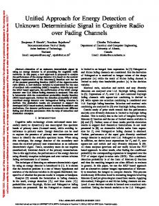
The block-flat fading single-user MIMO system is characterised by a flat-fading channel matrix H of size nR ×nT , which changes independently from block to block and the additive noise vector n at the receiver. Figure (1.1) shows the corresponding block diagram.

Figure 1.1: Block flat-fading MIMO system. In figure (1.1), the transmitted vector x is multiplied by the flat-fading channel matrix H and then the noise vector is added. The received signal is given by1 y = Hx + n.

(1.2)

In this model, the channel matrix H as well as the noise n is a random entity. The input dimension of the MIMO system equals the number of transmit antennas and is given by nT . The number of output dimensions of the MIMO systems equals the number of receive antennas and is given by nR 2 . The model depends on the propagation scenario, i.e. on the distribution of H. Well established models are the Rayleigh channel, i.e. the multipath environment without a line of sight (LOS) component in which H is modelled as zero-mean independent identically distributed (iid) complex Gaussian, i.e. H ∼ CN(0, I) or the Rice channel with a LOS component H ∼ CN(K, I) with constant LOS matrix K. The mutual coupling between the transmit and receive antennas can be modeled by correlation matrices [GBGP02, Mol04]. Possible singularities within the channel, are described as ’key-holes’ [CFGV02]. All quantities in (1.2) the transmit vector x, the received vector y, the noise vector n, and the channel matrix H are random variables with proper probability density functions (pdf). The mutual information between y and x under the assumption that the receiver side knows the channel realization H is given by I(y; x|H) = h(y|H) − h(y|H, x) = h(y|H) − h(n).

(1.3)

Throughout the whole thesis, the receiver is assumed to know the channel state H perfectly. CSI at the receiver is achieved either by channel estimation using pilot signals or by blind channel estimation. The differential entropy of the noise vector n in (1.3) depends on the pdf of the random variable n. Thermal receiver 1 In

order to keep notation simple, we omit the block index. signal model for flat-fading MIMO channels in (1.2) can be easily extended to frequencyselective channels by increasing the input and output dimensions of the MIMO system.

2 The

3

1 Introduction noise is modelled as a zero-mean complex Gaussian variable, i.e. n ∼ CN(0, σn2 I). Therefore, the entropy of the random noise vector is given by [CT91, Theorem 9.6.5]3

(1.4) h(n) = log (2πe)nR det σn2 I .

The entropy of the received vector y in (1.3) depends on the pdf of the input vector x. The transmitter chooses the pdf of x in order to maximise the mutual information. The largest entropy is achieved for zero-mean complex Gaussian distributed random variables. Therefore, the transmitter chooses x ∼ CN(0, Q) with transmit covariance matrix Q. Note that the random variables x and n are independent. As a result, the received vector for fixed channel realization H is zero-mean complex Gaussian distributed with receive covariance matrix W = σn2 I + HQH H . This follows from the fact that a linear combination of Gaussian random variables stays Gaussian and that the sum of independent zero-mean Gaussian variables is Gaussian distributed with zero-mean and covariance matrix which is the sum of the individual covariance matrices. Therefore, the conditional entropy of the received vector y is given by log ((2πe)nR detW )    = log (2πe)nR det σn2 I + HQH H .

h(y|H) =

(1.5)

Finally, from the entropy in (1.4) and the conditional entropy in (1.5) follows the instantaneous mutual information of the MIMO system in (1.2) with ρ = σ12 n





f (Q, H, ρ) = I(y; x|H) = log det I + ρHQH H .

(1.6)

The instantaneous mutual information is a function of the transmit covariance matrix Q, the channel realization H, and the inverse noise variance ρ. Often, we will normalise the transmit power to one, i.e. tr Q = P = 1. Then, ρ corresponds directly to the signal-to-noise-ratio (SNR). The mutual information in (1.6) depends on the channel realization H and is therefore a random entity. The instantaneous mutual information has been derived and analysed in the seminal work of Telatar [Tel99] and Foschini and Gans [FG98]. The equation (1.6) corresponds exactly to the result of the alternative derivation in [Tel99, Section 3.2] and to the derivation in the appendix of [FG98]. Finally, the expression in (1.6) can be maximised with respect to Q under a sum power constraint in order to get the instantaneous channel capacity of the MIMO system, i.e. c(ρ, H) =

max

Q: tr Q≤P

f (Q, H, ρ).

(1.7)

The channel capacity gives the upper bound of information which can be transmitted over the MIMO channel with arbitrary small probability of error if the channel is in state H. The instantaneous mutual information in (1.6) as well as the instantaneous channel capacity in (1.7) are random variables because they depend directly on the channel realization H. In order to get an average expression about the mutual information and the channel capacity which can be achieved, the expectation 3 Note,

that the factor 1/2 in front of the differential entropy in [CT91] vanishes if complex random variables are considered.

4

1.3 Performance metrics and preliminaries with respect to H is computed in order to obtain the average mutual information   (1.8) F (Q, ρ) = EH log det I + ρHQH H and to obtain the average channel capacity C(ρ) = EH

max

Q: tr Q≤P

f (Q, H, ρ).

(1.9)

If the random fading process H fulfils the ergodic property, the quantity C(ρ) in (1.9) is the ergodic channel capacity of the MIMO system. Interestingly, another performance metric is closely related to the average mutual information and to the channel capacity of the MIMO system: the mean square error (MSE). For computing these upper bounds on the achievable transmission rate with arbitrary small probability of error, the receiver applies the optimum detector and decoder. The optimum receiver algorithm is either the maximum likelihood (ML) or maximum a-posteriori (MAP) algorithm. However, capacity also can be achieved by decision feedback minimum mean square error (MMSE) detection [VG97]. The linear MMSE receiver reduces the computational complexity at the receiver side. If we apply the linear MMSE receiver, the performance metric changes from the average mutual information to the normalised MSE [VAT99]. The linear MMSE receiver weights the received signal vector y by the Wiener filter h i−1 ˆ = ρH H I + ρHQH H x y.

The covariance matrix of the estimation error K ǫ is given by i h H x − x) (ˆ x − x) K ǫ = EH (ˆ

(1.10)

(1.11)

The normalised MSE is defined as the trace of the normalised covariance matrix of the estimation error in (1.11) [HB03, JB03d]   mse(σn2 , Q, H) = tr Q−1/2 K ǫ Q−1/2  h i−1  H H = nT − tr ρHQH I + ρHQH (1.12) and its average over channel realizations is called normalised average MSE. It is given by  i−1  h (1.13) M SE(σn2 , Q) = nT − EH tr HQH H σn2 I + HQH H

1.3.2 Multiuser systems: Sum performance metrics The instantaneous performance metrics from the single-user analysis can be directly transfered to the multiuser case. However, in multiuser systems, the transmission from one user is disturbed by interference from the other users. In general, there are two possible multiuser scenarios: In the uplink, multiple users want to transmit their data to one common base station. The uplink is called the multiple access channel (MAC). In the downlink, the base transmits data to multiple users. This is called the broadcast channel (BC). The communication channel between each user

5

1 Introduction and the base is assumed to be block-flat fading.

Multiple access channel In the MAC, K users transmit their data simultaneously to the base station. All mobiles have nT transmit antennas4 . The received vector is given by y=

K X

H k xk + n.

k=1

The mutual information for user k according to the definition in section 1.3.1 under the assumption that the receiver knows the channel realization H k is given by ! K X H l Ql H H I(y; xk |H k ) = log det I + ρ l l=1



− log det I + ρ

K X

l=1,l6=k



 H l Ql H H l

(1.14)

with SNR ρ and transmit covariance matrices Qk . The transmit signals of the users are assumed to be zero-mean independent complex Gaussian distributed with covariance matrix Qk . This pdf maximises the individual mutual information of each user. Obviously, the individual mutual information of user k depends on the multiuser interference and noise, i.e. it is a function of all transmission channels H k between the users and the base, the SNR ρ and the transmit strategies Qk of all users ! PK I + ρ l=1 H l Ql H H l (1.15) Rk (Q, H, ρ) = log det PK I + ρ l=1,l6=k H l Ql H H l

with the set of covariance matrices Q and the set of channel realisations H Q = {Q1 , Q2 , ..., QK } and H = {H 1 , H 2 , ..., H K }.

The achievable rate of user k is denoted by Rk . It is possible, that the receiver first detects the signals of a set of users and subtracts them from the received signal before detecting user k. As long as the users transmit at a rate smaller than or equal to their mutual information, their signals are detected with arbitrary small probability of error and therefore correctly subtracted. Let us assume that the signals of users 1 to k − 1 are correctly subtracted, then the individual mutual information of user k is given by ! PK H I + ρ H Q H l l l l=1 RkSIC (Q, H, ρ) = log det . (1.16) PK I + ρ l=k+1 H l Ql H H l

The receiver starts with user one, detects his data, and subtracts it from the received signal. The received signal for user one is interfered by all other users. Then the second user is detected and subtracted. The second user gets interference from all but the first user. This procedure continues until the last user is detected without any interference. This approach is called successive interference cancellation (SIC). 4 It

is easy to generalize the results to the general case in which each mobile has a different number of transmit antennas.

6

1.3 Performance metrics and preliminaries Usually, one assumes that the data of all users is detected without errors because the users transmit with rate below their capacity. If we assume that the receiver detects the user signals in a linear fashion, the optimal choice is the linear multiuser MMSE receiver. The corresponding performance metric is the individual normalised MSE of user k which is given by  !−1  K X . (1.17) H l Ql H H M SEk = nT − tr ρH k Qk H H ρ k l +I l=1

In contrast to the capacity, it is not possible to perform SIC without error propagation, because the argument with the error free reception is missing. Therefore, each user k experiences interference from all other users. The achievable MSE region is given by all MSE tuples (m1 , ..., mK ) for which (m1 ≥ M SE1 , ..., mK ≥ M SEK ) applies.

Using the individual rate or the individual MSE, each user can require its qualityof-service (QoS) by giving a minimum rate rk or a maximum MSE mk which has to be achieved. The problem of the fulfilment of service requirements consists of computing a transmit strategy which ensures for all 1 ≤ k ≤ K that Rk ≥ rk or PKM SEk ≤ mk by minimising the individual pk ≤ Pk or sum transmit power k=1 pk ≤ P . Another performance metric is the sum of the individual performance metrics. The sum capacity is simply defined as the sum of the individual capacities K X

RkSIC (Q, H, ρ) ,

k=1

i.e. with SIC, we obtain C(Q, H, ρ) = log det I + ρ

K X

H k Qk H H k

k=1

!

.

The normalised sum MSE is defined in the same manner, i.e. M SE =

(1.18) K P

M SEk

k=1

and it is given by " #−1  nT X . H k Qk H H M SE(Q, H, ρ) = KnT − nR + tr  ρ k +I

(1.19)

k=1

The sum capacity and the sum MSE describe the performance of the complete MAC. The system throughput can be measured by the sum capacity in (1.18) or by the sum MSE (1.19). Broadcast channel In the MIMO BC scenario, we study the downlink transmission from the base station to the mobiles. The transmission channels between the base and the mobiles are reused from the MAC and by reciprocity5 we obtain the received vector at mobile 5 The

author in [Tel99] calls reciprocity the fact that the capacity is unchanged if the role of transmitter and receiver is interchanges in a MIMO point-to-point link. In our context, we assume that the uplink and downlink channels are reciprocal because the same frequency is

7

1 Introduction terminal k as yk =

K X

HH k xl + nk .

(1.20)

l=1

The achievable rate for user k under the assumption that the transmit signals intended for all users are zero-mean complex Gaussian distributed with covariance matrix Qk is given by ! PK I + ρ l=1 H k Ql H H k . (1.21) Sk (Q, H, ρ) = log det PK I + ρ l=1,l6=k H k Ql H H k

The counterpart to SIC at the base station in the MAC, is Costa-Precoding [Cos83]. It is possible, to subtract the already coded data for users 1 to k − 1 before encoding the data intended for user k without power increase. Therefore, user k receives only interference from users k + 1 to K. The achievable rate with Costa-Precoding for user k is given by ! PK I + ρ l=1 H k Ql H H k CST . (1.22) Sk (Q, H, ρ) = log det PK I + ρ l=k+1 H k Ql H H k

Achieving rate SkCST means that the base station performs Costa-Precoding, the transmit signals are all independent zero-mean complex Gaussian distributed, and the mobile performs optimal detection and decoding. The achievable sum rate of the MIMO BC with Costa-Precoding equals the sum capacity of the MIMO MAC. Furthermore, it can be shown by Sato’s bound [Sat78], that the achievable sum rate of the MIMO BC is the sum capacity itself. Therefore, the sum capacity of the MIMO BC with Costa-Precoding can be achieved by solving the MIMO MAC sum capacity problem and then transforming the transmit covariance matrices as described in [VJG02b]. This simplifies the analysis of the sum performance in terms of the sum capacity, because up- and downlink can be treated together. The same transformation of transmit covariance matrices from MAC to the BC can be applied for sum MSE minimisation. Therefore, by solving the sum MSE minimisation problem for the uplink, the corresponding downlink problem is solved, too. This concludes the informal introduction of the performance metrics for the singleuser and multi-user MIMO system. In the next section, the contribution of this thesis is summarised and the structure is presented.

1.4 Outline of the thesis The contributions of this thesis are summarised in the following: The contribution of 2nd chapter consists of the following points: First, we present related work and classify our work. In section 2.2.1 we introduce our channel model. Another ingredient is a rigorous mathematical measure of correlation which is defined in section 2.2.2. We observe that the average performance of the single-user MIMO system can be written as the average trace of an arbitrary matrix-monotone function [Bha97]. used, e.g. in TDD modus.

8

1.4 Outline of the thesis This observation allows us to analyse different performance metrics as representatives of a much larger class of performance functions. The complete analysis is performed on this meta layer. All results of the average mutual information and the average MSE follow as corollaries. This observation is presented in section 2.3.1. Then, the following results are proven: • Optimum transmission strategies: In section 2.3.2, we justify the intuitive belief that equal power allocation is optimal without CSI at the transmitter even if the transmit antennas and receive antennas are correlated. This is done by considering the worst case transmit and receive correlation and showing that equal power allocation is most robust against that. For the case when the transmitter knows the transmit and receive correlation matrix6 , we show that the average performance is optimised by transmitting along the eigenvectors of the transmit correlation matrix. In addition to this, we characterise the optimum power allocation for the covariance feedback case and develop an iterative algorithm which solves the power allocation optimisation problem. At low SNR values only one eigenvalue is supported, i.e. the transmitter performs beamforming. The SNR range in which beamforming is optimal is characterised for arbitrary transmit and receive correlation and arbitrary average performance function. With perfect CSI at the transmitter, the transmit strategy is adapted to each channel realization. The MIMO channel is decomposed according to the singular value decomposition first, then optimal power across the parallel Gaussian channels is allocated. We derive the generalised water-filling solution. At low SNR, the beamforming range bases on a instantaneous channel realization is derived. • Impact of correlation on the ergodic capacity: In section 2.3.3, for an arbitrary number of transmit and receive antennas and for arbitrary SNR values we show that uncorrelated MIMO channels yield higher capacities than correlated channels with uninformed transmitter and a receiver which has perfect CSI. We show that the average performance of an open-loop MIMO system is a Schur-concave function with respect to transmit and receive correlation. In addition to this, the difference between the ergodic capacity of fully correlated and completely uncorrelated MIMO channels is studied and a tight lower bound is developed. For the case in which the transmitter knows the transmit correlation matrix, we show that the average performance can be either Schur-convex or Schurconcave or nothing with respect to transmit correlation depending on the SNR. For small SNR, beamforming is optimal. If beamforming is optimal, the average performance is Schur-convex with respect to transmit correlation. With respect to receive correlation, we show that the covariance feedback MIMO ergodic channel capacity is a Schur-concave function. The closed-loop MIMO average performance is shown to be Schur-convex with respect to transmit and receive correlation for small SNR values and Schurconcave at high SNR values. • Comparison to MISO results: In section 2.3.4, the differences between MIMO and MISO channels are analysed. The general structure of the optimum transmission strategies for the different types of CSI between MISO 6 This

case is called ’covariance feedback’, because the knowledge at the transmitter about the two covariance matrices can be achieved by channel estimation at the receiver and slow feedback to the transmitter.

9

1 Introduction and MIMO systems corresponds well. However, the impact of correlation on MISO and MIMO systems substantially differs. In MISO systems much stronger results can be proven. The average MISO covariance feedback performance is Schur-convex with respect to transmit correlation. The average closed-loop MISO performance is Schur-concave with respect to transmit correlation. As a result, the average performance for the complete set of types of CSI is analysed. In a clearly arranged table, we give a complete summary of all theoretical results. • Illustration and discussion of average performance results: In section 2.3.6, the theoretical results from the last sections, are summarised by illustrative numerical simulations. The properties of the different average performance metrics under correlation and under the different types of CSI can be read off. In chapter 3, multi-user multiple-antenna systems and their respective performance metrics are studied. We start with a point-to-point link which experiences noise, inter-cell interference and intra-cell interference. We incooperate these three fractions into the noise with specific noise covariance matrix. We compute the worst case noise performance of the MIMO link in three different noise scenarios. The contributions of the worst case noise analysis in section 3.2 are: • The performance of a MIMO closed-loop system, i.e. perfect CSI at the transmitter, with worst case noise under a trace constraint (or worst case interference) equals the performance of a MIMO open-loop system, i.e. no CSI at the transmitter with white noise, i.e. without interference. The structure of the equivalent system is a single-user MIMO system with uncorrelated noise and without CSI at the transmitter. We do a complete characterisation of the solution of the corresponding minimax expression. • The worst case noise directions correspond with the left eigenvectors of the channel matrix H. The optimal transmit directions correspond with the right eigenvectors of the channel matrix H. Both are independent of each other. Therefore, the minimax problem fulfils the saddle point property. The power allocation then is the well-known waterfilling solution. • The worst case coloured noise decomposes the closed-loop MIMO system into a SIMO MAC with amplified white noise. The transmitter cooperation goes loose and the noise is amplified by a factor equal to the number of receive antennas. Furthermore, in section 3.3, we explicitly incooperate all transmit strategies into the optimisation of the sum performance of the multiuser MIMO system. The sum performance can be the sum capacity of the MIMO MAC if SIC is applied or the sum capacity of the MIMO BC if Costa Precoding is applied or the sum MSE of the MAC. We assume perfect CSI at transmitter and mobiles and derive the optimal transmit strategies under individual and sum power constraints. The structure of this part of the thesis is summarised in the following: • At first, the signal model and the associated performance metrics are introduced in section 3.3.1. The problem statements are proposed in section 3.3.2. The sum performance is maximised under a sum power constraint. • We solve these problems in section 3.3.3 and derive an iterative algorithm which efficiently solves the sum performance optimisation problem of the multiuser MIMO system. We show that the original problem can be decomposed into two parts, namely power allocation and covariance matrix optimisation under individual power constraints. These two parts are alternately

10

1.4 Outline of the thesis performed and converge to the optimal solution. Furthermore, the covariance matrix optimisation step can be further decomposed into iterative single-user performance optimisation treating the other users as noise. • In order to get better understanding of the optimal transmit strategy which is in general very complex, we analyse the strategy at low SNR values in section 3.3.4. We completely characterise the SNR range, in which only one user is allowed to transmit at a time. • This chapter is concluded in section 3.3.5 by a short discussion of the construction of the iterative algorithm. In addition, we provide an illustrative example of average sum capacities for SISO, SIMO, and MIMO MACs with different numbers of users and SNR values. Finally, in chapter 4, we conclude the thesis and give directions for further research. The list of publications and the bibliography finalise this thesis.

11

1 Introduction

12

2 Optimal transmission strategies and impact of correlation in single-user multiple-antenna channels 2.1 Related work The increasing need for fast and reliable wireless communication links has opened the discussion about systems with multiple antennas both located at the transmitter and the receiver - so called multiple-input multiple-output (MIMO) systems [FG98]. Systems with multiple antennas at one side of the link are well known [Jak74] for increasing the capacity and performance. In recent years, it was discovered that MIMO systems have the ability to reach higher transmission rates than one-sided array links [WFGV98] [Tel99]. Many results regarding the capacity of MISO and MIMO systems under different levels of CSI and the corresponding transmission strategies were recently published. First, we review recent results for MISO systems. The MISO case has recently attracted much attention. In [Win98], the potential of multiple antenna systems was pointed out. The capacity of a MISO system with imperfect feedback was first analysed in [VM01] and [NLTW98, NTW99]. In [JG01b, JB02b] the optimum transmission strategy with covariance knowledge at the transmit array with respect to the ergodic capacity was analysed. In [RFLT98, SB01, BS01], the problem of downlink beamforming in MISO systems was solved. In [JG03], the ergodic capacity in the non-coherent transmission scenario with only covariance knowledge at the transmitter and the receiver, is studied. It has been shown that even partial CSI at the transmitter can increase the capacity of a MISO system. Recently, transmission schemes for optimising capacity in MISO mean-feedback and covariance-feedback systems were derived in [VM01, NLTW98]. The capacity can be achieved by Gaussian distributed transmit signals with a particular covariance matrix. In a block fading model, the general signal processing structure which achieves capacity independent of the type of CSI consists of a Gaussian codebook, a number of beamformers and a power allocation entity [VM01, BCT01]. Additionally, it has been proved that the optimal transmit covariance matrix in the covariance feedback case has the same eigenvectors as the known channel covariance matrix. The complete characterisation of the impact of correlation on the ergodic capacity in MISO systems can be found in [JB04c]. While studying MIMO systems, we can imagine several different scenarios in which the transmitter or the receiver have partial or perfect channel state information (CSI). The capacity of a single-user MIMO system with perfect CSI at the receiver and no CSI at the transmitter was studied in [Tel99]. Equal power allocation was shown to be optimal for uncorrelated Rayleigh fading MIMO channels without CSI at the transmitter. The optimum strategy in order to minimise the outage probability is analysed in [JB03a]. The capacity of a single-user MIMO system with perfect CSI at both the transmitter and the receiver can be derived from the ’water-filling’ approach [CT91, Tel99]. If the transmitter has only partial CSI in terms of the channel covariance matrix the optimal transmission strategy is shown in [JG01b] to transmit in the direction of the known channel eigenvectors. The power allocation problem is discussed in [JG01b], [JB02a], [SM02] and [JB02b].

13

2 Single-user multiple-antenna optimisation Practical power allocation and rate adaption algorithms are discussed in [MBO04, BMO04]. The case in which both the transmitter and the receiver do not have channel state information remains an open problem. Even for the single-input single-output Rayleigh fading case, the capacity achieving transmission strategy for no CSI has not been solved completely [AFTS01]. For MIMO case, the optimum transmission strategy without CSI at the transmitter and receiver was characterised in [MH99].

Most of the results regarding the ergodic and outage capacity of single user MISO and MIMO systems assume that the transmit and receive antennas are uncorrelated. In reality, there can occur correlation at the transmit antenna array due to the placement of the array and the geometry in the transmission scenario. Especially at the base station which is often un-obstructed, correlation between the antennas can occur.

In literature there are different models which measure the correlation of the transmit and receive antennas in MIMO systems. We use the well established model from [CTK02]. This model is well suited for Rayleigh and Ricean MIMO channels which naturally arise in a rich scattering environment. In [SFGK00] a model for correlation of the multi element antenna was developed and the ergodic and outage capacity was computed under correlation. In [CTK02] the impact of correlation was analysed by studying the asymptotic eigenvalue distribution of the channel matrix for a large number of transmit and receive antennas. The theory of majorization for discrete vectors was extended to continuous probability density functions and it was shown that correlation decreases the ergodic capacity. In [MO02], an approximative expression for the capacity of correlated MIMO channels has been presented. In [MSS01] analytical results for the moments of the mutual information under correlation were derived for large antenna arrays, too. Using the tight capacity bound which was developed in [ONBP02] for high SNR values, the impact of correlation can easily be analysed. All analytical results assume either a large number of antennas or high SNR values. Although the recent results indicate that correlation decreases the ergodic capacity without CSI at the transmitter, the general proof is still missing. For the MISO case, a proof was derived in [BJ04a]: The ergodic capacity of a MISO system with no CSI at the transmitter decreases if the transmit correlation increases. Furthermore, it was shown in [BJ04a], that the capacity loss due to correlation is bounded by some small constant.

The statistics in MIMO channels are entirely characterised by the transmit and receive correlation matrix if the channel between is a rich scattering channel which is assumed Rayleigh distributed. If the channel between the transmit and receive array has singularities or rank deficiencies, the channel statistics are more complex. A method for describing such phenomena was proposed in [Say02]. The analysis in [CFV00, CFGV02] is adapted to several special practical scenarios in which so called keyholes occur. For example, in indoor transmission scenarios in which we have long corridors the channel can be singular. This is not because of correlation at the transmitter or the receiver but because of a keyhole in between. We do not discuss effects like keyholes in this thesis, because we study the impact of correlation of the transmit antenna array separately. Therefore, we assume that the channel between transmitter and receiver does not have keyholes.

14

2.2 Channel model and basic definitions

2.2 Channel model and basic definitions 2.2.1 Channel model Consider the standard MIMO block flat-fading channel model y = Hx + n

(2.1)

with complex nT × 1 transmit vector x, channel matrix H with nR × nT entries, σ2 circularly symmetric complex Gaussian noise n with variance 2N I per dimension. 2 For convenience, we define the inverse noise variance as ρ = 1/σN . We assume that the receiver knows H perfectly. Let us first describe the signal processing at the transmit antenna array. The transmit covariance matrix is given by
Q = E xxH .

Using the eigenvalue decomposition of Q = U Q ΛQ U H Q , it becomes obvious how one can construct a particular transmit covariance matrix. The input data stream d(k) is split into m parallel data streams d1 (k) . . . dm (k). Each parallel data stream √ √ is multiplied by a factor p1 . . . pm and then weighted by a beamforming vector u1 . . . um . The number of parallel data streams is less than or equal to the number of transmit antennas (m ≤ nT ). The beamforming vectors ui have size nT × 1 with nT as the number of transmit antennas. The powers p1 , ..., pnT correspond to the eigenvalues in the diagonal matrix ΛQ . The nP T signals of each weighted data stream √ m xi (k) = di (k) · pi · ui are added up x(k) = i=1 xi (k) and sent. By omitting the time index k for convenience we obtain in front of the transmit antennas x=

m X l=1

dl ·

√

pl · ul .

(2.2)

The signal processing structure is shown in figure (2.1). The transmit signal in x has

d1(k) d(k)

1 u

x

1

λ1

S/P

+

y (k) 1

x (k) 1

nT MIMO Channel

y (k) 2

1

1:m d (k) m

x λm

u m

nT

+

x (k) nT

y (k) nR

Figure 2.1: Signal processing structure for the MIMO system. a covariance matrix Q with eigenvalues p1 , ..., pm , 0, ..., 0 and eigenvectors u1 , ..., um . In order to construct a transmit signal with a given covariance matrix, two signal processing steps are necessary: The first step is the power control p1 , ..., pm and the second step is multiplying the beamformers u1 , ..., um . The sum transmit power

15

2 Single-user multiple-antenna optimisation PnT

k=1

pk is constrained, i.e. nT X

pk = P.

k=1

Next, we study the stochastic properties of the channel. The correlation of the channel vectors arises in the common downlink transmission scenario in which the base station is un-obstructed [SFGK00]. We follow the model in [GP94] where the subspaces and directions of the paths between the transmit antennas and the receive cluster change more slowly than the actual attenuation of each path. The channel matrix H for the case in which we have correlated transmit and correlated receive antennas is modelled as 1

1

H = RR2 · W · RT2

(2.3)

with transmit correlation matrix RT = U T D T U H T and receive correlation matrix . U and U are the matrices with the eigenvectors of RT and RR = U R D R U H T R R RR respectively, and D T , D R are diagonal matrices with the eigenvalues of the matrix RT and RR , respectively. The random matrix W has zero-mean independent complex Gaussian identically distributed entries, i.e. W ∼ CN(0, I). The most general form of the correlation model consists of a very large correlation matrix of size (nT · nR × nT · nR ) which incooperates the transmit and receive correlation, i.e. it is the expectation of the outer product of the vectorised channel matrix   κ = E vec(H) · vec(H)H . (2.4) The correlation matrix κ in (2.4) expresses the correlation between each transmit or receive element to every other transmit or receive element. Often, the transmit and the receive antenna array are spatially divided. Then, the following simplification is allowed [CTK02]. In the case in which each receive antenna observes the same correlation between the transmit antennas, i.e. the transmit correlation is independent of the receive antenna and vice versa the receive correlation is independent of the transmit antenna, the correlation model in (2.4) simplifies in comparison to the model in (2.3).

We assume that the entries in the channel matrix are complex Gaussian distributed. Therefore, we can describe the impact of the correlation at the transmitter and the receiver by considering the second moment, i.e. the covariance matrix. The analysis in [CFV00, CFGV02] can not be applied to our scenario because the entries of the channel matrix in [CFV00, CFGV02] are products of complex Gaussian distributed entries. It does not suffice to consider only the second moment in order to analyse the impact of correlation or keyholes. However, the authors in [CFV00, CFGV02] argue that a MIMO system with ’many’ keyholes converges to the common MIMO model by application of the central limit theorem. The model of correlation which we introduced in (2.3) allows to analyse the different performance metrics from chapter 1 with respect to correlation at the transmit and the receive side. In order to provide a stable mathematical theory for studying correlation, we give a mathematical measure of correlation in the next section.

16

2.2 Channel model and basic definitions 2.2.2 A mathematical measure of correlation In order to provide a measure of correlation, we take two arbitrarily chosen transmit correlation matrices R1T and R2T with the constraint that trace(R1T ) = trace(R2T ) = nT which is equivalent to nT X

λT,1 = l

l=1

nT X

λT,2 l ,

(2.5)

l=1

with λlT,1 , 1 ≤ l ≤ nT , and λT,2 l , 1 ≤ l ≤ nT , are the eigenvalues of the covariance matrix R1T and R2T , respectively. This constraint regarding the trace of the correlation matrix RT is necessary because the comparison of two transmission scenarios is only valid if the average path loss is equal. Without receive correlation, the trace of the correlation matrix can be written as nT  h nT i X X   H trace(RT ) = E HH = E |hi |2 . ii

i=1

(2.6)

i=1

However, the RHS of (2.6) is the sum of the average path loss from the transmit antenna i = 1...nT . In order to study the impact of correlation on the achievable capacity separately, the average path loss is kept fixed by applying the trace constraint on the correlation matrices R1T and R2T . We will say that a correlation matrix R1T is more correlated than R2T with descendT,2 ing ordered eigenvalues λT,1 ≥ λT,1 ≥ ... ≥ λT,1 ≥ λT,2 ≥ ... ≥ λT,2 nT ≥ 0 and λ1 nT ≥ 1 2 2 0 if m X

k=1

λT,1 ≥ k

m X

k=1

λT,2 1 ≤ m ≤ nT − 1. k

(2.7)

The measure of correlation which we will introduce is defined in a natural way: the larger the first m eigenvalues of the correlation matrices are (with the trace constraint in (2.6)), the more correlated is the MIMO channel. As a result, the most uncorrelated MIMO channel has equal eigenvalues, whereas the most correlated MIMO channel has only one non-zero eigenvalue which is given by λ1 = nT . Before proceeding with our definition of ’more correlated’ in terms of the eigenvalue distribution of the channel covariance matrix, we give the necessary definitions we will need in the following. Definition 1: For two vectors x, y ∈ Rn with descending ordered components x1 ≥ x2 ≥ ... ≥ xn ≥ 0 and y1 ≥ y2 ≥ ... ≥ yn ≥ 0 one says that the vector x majorizes the vector y and writes x ≻ y if

m X

k=1

xk ≥

m X

k=1

yk , m = 1, ..., n − 1. and

n X

k=1

xk =

n X

yk .

k=1

The next definition describes a function Φ which is applied to the vectors x and y with x ≻ y: Definition 2: A real-valued function Φ defined on A ⊂ Rn is said to be Schur17

2 Single-user multiple-antenna optimisation convex on A if x ≻ y on A ⇒ Φ(x) ≥ Φ(y). Similarly, Φ is said to be Schur-concave on A if x ≻ y on A ⇒ Φ(x) ≤ Φ(y).

n Example: Suppose that x, y ∈ R+ are positive real numbers and the function Φ is defined as the sum of the squared components of the vectors, i.e. Φ2 (x) = Pn 2 n |x | . Then, it is easy to show that the function Φ2 is Schur-concave on R+ , k k=1 i.e. if x ≻ y ⇒ Φ2 (x) ≤ Φ2 (y).

We will need the following lemma (see [MO79, Theorem3.A.4]) which is sometimes called Schur’s condition. It provides an approach for testing whether some vector valued function is Schur-convex or not. Lemma 1: Let I ⊂ R be an open interval and let f : In → R be continuously differentiable. Necessary and sufficient conditions for f to be Schur-convex on In are f is symmetric on In

(2.8)

and (xi − xj )



∂f ∂f − ∂xi ∂xj



≥ 0 forall 1 ≤ i, j ≤ n.

(2.9)

Since f (x) is symmetric, Schur’s condition can be reduced as in [MO79, p. 57]   ∂f ∂f (x1 − x2 ) ≥ 0. (2.10) − ∂x1 ∂x2 From Lemma 1 follows that f (x) is a Schur-concave function on In if f (x) is symmetric and   ∂f ∂f (x1 − x2 ) − ≤ 0. (2.11) ∂x1 ∂x2 The definition of Schur-convexity and Schur-concavity can be extended if another function Ψ : R → R is applied to Φ(x). Assume that Φ is Schur-concave, if the function Ψ is monotonically increasing then the expression Ψ(Φ(x)) is Schurconcave, too. If we take for example the function Ψ(n) = log(n) for n ∈ R+ and the function Φp from the example above, we can state that the composition of the two n functions Ψ(Φp (x)) is Schur-concave on R+ . This result can be generalised for all possible compositions of monotonically increasing as well as decreasing functions, and Schur-convex as well as Schur-concave functions. For further information about majorization theory see [MO79]. The following definition provides a measure for comparison of two correlation matrices. Definition 3: The transmit correlation matrix R1T is more correlated than R2T if

18

2.2 Channel model and basic definitions and only if m X l=1

λT,1 l

≥

m X

λT,2 l

for m = 1...nT , and

l=1

nT X l=1

λT,1 1

=

nT X

λT,2 2 .

(2.12)

l=1

One says that the vector consisting of the ordered eigenvalues λT1 majorizes λT2 , and this relationship can be written as λT1 ≻ λT2 like in Definition 1. Remark I: It can be shown that vectors with more than two components cannot be totally ordered. So there are examples of correlation vectors that cannot compared using our Definition 3, e.g. η 1 = [0.6, 0.25, 0.15] and η 2 = [0.55, 0.4, 0.05]. This is a problem of all possible orders for comparing correlation vectors. Majorization induces only a partial order. Note that our definition of correlation in Definition 3 differs from the usual definition in statistics. In statistics a diagonal covariance matrix indicates that the random variables are uncorrelated. This is independent of the auto-covariances on the diagonal. In our definition, we say that the antennas are uncorrelated if in addition to statistical independence, the auto-covariances of all entries are equal. This difference to statistics occurs because the direction, i.e. the unitary matrices of the correlation have no impact on our measure of correlation. Imagine the scenario in which all transmit antennas are uncorrelated, but have different average transmit powers because of their amplifiers. In a statistical sense, one would say the antennas are uncorrelated. Our measure of correlation says that the antennas are correlated, because they have different transmit powers. The measure of correlation in Definition 3 is more suitable for the analysis of the performance of multiple antenna systems, because different transmit powers at the antennas obviously have a strong impact on the performance. In this thesis, these effects are considered. This measure of correlation allows us to analyse the impact of correlation on the various performance metrics introduced in chapter 1 in single-user MIMO systems under different types of CSI. In the following, the measure of correlation is applied to transmit correlation matrices RT and to receive correlation matrices RR as well. Remark II: As mentioned above, the case in which the transmit antennas are fully correlated corresponds to λT1 = nT , λT2 = ... = λTnT = 0. The case in which the transmit antennas are fully uncorrelated corresponds to λT1 = λT2 = ... = λTnT = 1. This illustrates that the expression in (2.12) can be used as a measure for correlation. Example: At this point, we give another example for the measure of correlation. Assume the situation in figure (2.2). We have two different correlation scenarios. B A B In scenario A and B the largest two eigenvalues (λA 1 = λ1 and λ2 = λ2 ) are equal. B B The smallest three eigenvalues in scenario B are equal (λ3 = λ4 = λB 5 ) but in A A scenario A the smallest three eigenvalues are unequal (λA > λ > λ ). In addition 3 4 5 to this, the sum of all eigenvalues in scenario A and B is equal. Applying the order which is introduced in Definition 3, eigenvalue vector A majorizes eigenvector B (λA ≻ λB ). Scenario B applies for all eigenvalue distributions λ with fixed λ1 and λ2 and equal trace the ’smallest’ eigenvalue distribution, i.e. λB ≺ λ for all λ with λ1 + λ2 +

nT X

λk = 1

k=3

19

2 Single-user multiple-antenna optimisation

Scenario A λ1

λ2

Scenario B λ3

λ4

λ5

λ1

λ2

λ3

EIGENVALUES

λ4

λ5

EIGENVALUES

Figure 2.2: Example correlation matrix eigenvalue distribution. and for λB with B 1 − λB 1 − λ2 B = λB 3 = ... = λnT . nT − 2

Entropy of Gaussian vector As another example of the measure of correlation, consider a random Gaussian distributed vector z of dimension n with z ∼ CN (0, R) and with covariance matrix R. Denote the eigenvalues of the covariance matrix R as r = [r1 , ..., rn ]. In the following, we show that the entropy hr (z) is a Schurconcave function with respect to the correlation eigenvalues r. The entropy of z is given by [CT91, Theorem 9.6.5] # " n Y n n (2.13) hr (z) = log [(2πe) det(R)] = log (2πe) ri . i=1

Further on, we have the following result by [MO79, Theorem 3.F.1.a] λ≻µ→

n Y

i=1

λi ≤

n Y

µi .

(2.14)

i=1

Therefore, from (2.13) and (2.14) follows λ ≻ µ → hλ (z) ≤ hµ (z). This can be shown alternatively, by # " n n X Y n n log ri . hr (z) = log (2πe) ri = log(2πe) +

(2.15)

i=1

i=1

According to [MO79, Proposition 3.C.1], λ≻µ→

n X i=1

log λi ≤

n X

log µi .

i=1

2.3 Average performance metrics We assume that the receiver has perfect CSI. The transmitter has either no CSI, perfect CSI, or knowledge of the transmit correlation matrix RT and receive correlation matrix RR . Let us study the optimisation problems regarding the average

20

2.3 Average performance metrics performance metrics average mutual information (1.8) and average normalised MSE (1.13) from chapter 1. All average performance metrics introduced in chapter 1 can be written in the following generalised form 1/2

1/2

1/2

1/2

Φ(ρ, Q, RT , RR ) = EW tr φ(ρRR W RT QRT W H RR )

(2.16)

with zero-mean complex Gaussian iid random matrix W and with the matrix-valued function φ defined on the set of positive semidefinite matrices. Using the following matrix-valued function φ1 (X) in the RHS of (2.16) φ1 (X) = log (I + X)

(2.17)

the generalised average performance function Φ in (2.16) corresponds in every detail to the average mutual information in (1.8). Using another matrix-valued function φ2 (X) in (2.16) φ2 (X) =

nT −1 I − X [I + X] nR

(2.18)

the function Φ in (2.16) directly corresponds to the average normalised MSE in (1.13). The average normalised MSE is to be minimised. The first term in the RHS of (2.18) does neither depend on the transmission strategy nor on the transmit or receive correlation. It depends only on the number of transmit and receive antennas. Therefore, the minimisation of the normalised average MSE can be expressed as a maximisation of the function −1 φ˜2 (X) = X [I + X]

(2.19)

In (2.16) it is assumed that the transmit signals are complex Gaussian distributed with transmit covariance matrix Q with power constraint tr (Q) = P . The transmit covariance matrix can be understood as an operator that maps from the set of all channel matrices H = {H} to the set of transmit covariance matrices under the trace constraint Q = {Q : Q  0, tr Q = P }. The maximum of (2.16) with respect to transmit strategy Q depends on the CSI at the transmitter. In general, the generalised performance function Φ in (2.16) is optimised with respect to transmit policy Q under the trace constraint. As a result, for fixed SNR ρ, transmit RT and receive correlation matrices RR , we obtain the following class of optimisation problems max or min Φ(Q, ρ, RT , RR ) s.t. Q  0 and tr Q = P .

(2.20)

If the transmitter has perfect CSI, the transmitter can adapt its transmit strategy Q to every channel matrix realization H. The transmit strategy changes with every channel realization. In case of average mutual information maximisation, the optimal transmission strategy is the well known ’water-filling’ [Tel99], [CT91]. Then, the maximum mutual information corresponds to the ergodic channel capacity of a closed-loop MIMO system. In case of average normalised MSE minimisation, the optimal transmission strategy is some kind of altered ’water-filling’ [HB03]. In section 2.3.2, we derive the general structure of the optimal transmit strategy Q for arbitrary inner performance function φ. If the transmitter has knowledge about the transmit and receive correlation, the transmit strategy does not depend on each instantaneous channel realization. The

21

2 Single-user multiple-antenna optimisation transmit covariance matrix is kept fixed for a pair of transmit and receive correlation matrices. In order to describe the optimisation problem which leads to the optimal transmission strategy with covariance feedback, we discuss the expression in (2.16). The main problem in computing the average generalised performance metric Φ in (2.16) is the expectation operator. We obtain for the expectation of the inner matrix-valued function 1/2

1/2

1/2

1/2

1/2

1/2

EW tr φ(ρRR W RT QRT W H RR ) 1/2

1/2

= EW tr φ(ρΛR W ΛT QΛT W H ΛR ) ! nT X H T ˜k . ˜ kw λ k pk w = Ew1,...,nT tr φ ρ

(2.21)

k=1

The first identity in (2.21) follows from the fact that the distribution of the random variable W and W U and U W for unitary U are equal. This fact has been extensively used in [MH99]. Furthermore, note that the trace of U W U H is equal to the trace of W for unitary U . The random vectors w ˜ k for 1 ≤ k ≤ nT are given by p   R pλ1 w1,k   λR 2 w2,k     . (2.22) w ˜k =  .   q . λR nR wnR ,k

with zero-mean complex Gaussian iid random variables wi,j with 1 ≤ i ≤ nR and 1 ≤ j ≤ nT . Note that the LHS in (2.21) can be further rewritten as ! nR X 1/2 1/2 1/2 H H 1/2 R ˆk ˆ kw tr φ(ρRR W RT QRT W RR ) = tr φ ρ λk w (2.23) k=1

ˆ k for 1 ≤ k ≤ nR as with w   p T pp1 λ1 wk,1  p2 λT2 wk,2    . .. w ˆk =    .  q pnT λTnT wk,nT

(2.24)

The equations (2.21) and (2.23) express the symmetry of the average performance metric with respect to the correlation properties at the transmitter and the receiver. For the equal power allocation transmit strategy, one can observe that the impact of correlation at the transmit antennas or at the receive antennas is equal. This intuitive explanation will be affirmed in Corollary 7 and Theorem 3. In the case in which the transmitter knows the transmit correlation matrix and receive correlation matrix, the optimum eigenvectors of the transmit covariance matrix Q correspond to the eigenvectors of the transmit correlation matrix. This will be proven in section 2.3.2. For the average mutual information, this was shown in [JVG01] for completely uncorrelated receive antennas and in [JB03b] for receive correlation. The optimal power allocation is given by !!# " nT X opt λTi pi w ˜iw ˜H (2.25) max E tr φ ρ ΛQ = argp i n

P

T k=1

22

pk =P

i=1

2.3 Average performance metrics with w ˜ i given in (2.22). Using the optimum transmit strategy characterised so far, the maximum of the average mutual information (for φ1 in (2.25)) corresponds to the ergodic channel capacity of a MIMO system with long-term knowledge about the transmit and receive correlation. If the transmitter has no CSI, it can neither adapt the transmit strategy to the instantaneous channel realization nor to the long-term channel information. The transmit strategy is fixed for all channel realizations. Furthermore, it is difficult to define a channel capacity, because the average mutual information itself is a variable which depends on the transmit and receive correlation. In addition to this, it is not obvious how to define the best transmit strategy. What correlation should be assumed? In the next subsection, we propose an approach in order to solve these problems. We show that the optimal transmit covariance matrix which solves (2.20) under the worst case channel correlation (see section 2.3.2) is given by Qopt =

P I. nT

(2.26)

In the next section, we prove that equal power allocation as assumed in (2.26) is most robust against worst case correlation without CSI at the transmitter. Additionally, the solution to the optimisation problem in (2.20) is characterised and the well-known waterfilling solution for perfect CSI at the transmitter is briefly reviewed in the next section.

2.3.1 Properties of the inner matrix-valued performance function: Matrix-concavity Before proceeding to the next section, it is important to know the properties of the function φ in the optimisation problem (2.20). The following definitions will prove useful. Matrices and functions are discussed in [Bha97, HJ91]. The function F : Cn+ → Cn+ is a matrix-valued function. The function F maps from the set of positive semidefinite matrices to the set of positive semidefinite matrices. We consider only matrix-valued functions which act by a scalar function F (x) on each eigenvalue of the matrix A motivated by the spectral theorem in linear algebra. Therefore, the function F affects only the eigenvalues of the matrix A = U ΛU H , i.e. F (A) = U F (Λ)U H and F (Λ) = diag (F (λ1 ), ..., F (λn )). We will assume that F is matrix-monotone, i.e. F (A)  F (B) holds if A − B  0 [Bha97, Section V]. In our case the function φ1 (A) for the mutual information and ˜ (A) for the normalised MSE are matrix-monotone. the function φ 2 A matrix-valued function is matrix-concave if F [(1 − λ)A + λB]  (1 − λ)F (A) + λF (B).

(2.27)

A function F is called matrix-convex if −F is matrix-convex. Both performance functions φ1 (X) and φ2 (X) are matrix-concave and matrix-convex, respectively. Therefore, we restrict our analysis to the cases in which the inner function φ in the optimisation problem (2.20) are matrix-concave or matrix-monotone functions1 . Next, we define according to L¨ owner’s Theorem [L¨o34] [Bha97, Section V.4] the 1 In

[HP82, Theorem 2.5] it is shown that all operator monotone functions on (0, ∞) are operator concave.

23

2 Single-user multiple-antenna optimisation following class of matrix valued functions Z ∞ −1 ˜ (A) = sA (sI + A) dµ(s) F

(2.28)

0

with a positive measure µ ∈ [0, ∞), i.e. µ is monotonically increasing, positive, and continuous from the left [KF70], with entries Z ∞ h i i h −1 ˜ s A (sI + A) F (A) = dµ(s). (2.29) kl

kl

0

Every matrix-monotone function F can be expressed by a unique positive measure ˜ in (2.28) and (2.29) plus a constant term and a µ defined on [0, ∞] as the function F linear term. In this thesis, we consider only the class of matrix-monotone functions which can be expressed with the representation in (2.28). As a result, the optimisation problem in (2.20) can be expressed using L¨ owner’s representation of matrix-convex functions as Z ∞   1/2 1/2 1/2 1/2 s ρRR W RT QRT W H RR (2.30) Φ(ρ, Q, RT , RR ) = E tr 0

i−1  1/2 1/2 1/2 1/2 · sI + ρRR W RT QRT W H RR dµ(s). h

Note that the measure dµ(s) in (2.30) depends on the inner performance function φ. Often, the representation in (2.30) is useful for solving the optimisation problem (2.20) in the forthcoming sections. Note that the term inside the integral equals the second summand of the matrix-valued function φ2 . The integral and the trace operator can be interchanged because the trace is a finite sum. Often, we will need the first derivative of the matrix valued function F at A d DF (A)(H) = F (A + tH). dt t=0

There is an interesting relationship between the derivative DF (A) and the matrix F [1] (A). According to the approach in this section, it is defined in the following way: F [1] (A) acts on the eigenvalues of A = U ΛA U H with F [1] (A) = U diag(f ′ (λ1 ), f ′ (λ2 ), ..., f ′ (λn ))U H

(2.31)

Since the matrix F [1] (A) can be conveniently expressed using the positive measure µ, we will often use this matrix in the following. Let us call the matrix F [1] (A) the ’outer derivative’ of F . Examples of performance metrics of the matrix-monotone class In communications systems analysis, the performance of the system is often measured by a function which belongs to the aforementioned class, i.e. it can be represented as the trace of a matrix-monotone function with channel H and transmit strategy Q as an argument E tr φ(ρHQH H ). The average mutual information can be expressed as this type of function as shown above φ(X) = log det (I + ρX). The distribution µ(s) in the L¨ owner representation u(s−1) is then given by µ(s) = s2 with the step function u(t) = 0 for t < 0 and u(t) = 1 for t ≥ 0. 24

2.3 Average performance metrics −1

For the normalized MSE, the function φ is φ(X) = X [I + X] . In this case, the distribution µ(s) is given by µ(s) = δ(s − 1) with the dirac impulse δ(0) = 1 and otherwise δ(t) = 0 for t 6= 0. The Chernoff bound of orthogonal space-time block codes can be represented [NBP02] by taking the natural logarithm and φ(X) = log(nα )(−αX) with symbol constellation parameters nα as the number of signal point with minimum distance and α = ρ · dmin with SNR ρ and minimum distance dmin . 2.3.2 Optimum transmission strategies In this section, we derive the transmission strategies which maximise the average performance metrics for the single-user MIMO system in (2.20) with no CSI, covariance knowledge, and perfect CSI at the transmitter. Optimum transmission strategy without CSI at the transmitter In this section, we derive the optimum transmission strategy without CSI at the transmitter and with correlation at the transmit antenna array. In order to do so we have to introduce additional constraints on the transmit correlation matrix. In the following, we consider the least favourable transmit correlation matrix and search for the transmit strategy which maximises the average performance metric under this correlation matrix. This kind of min-max expression for the mutual information in the case in which the transmitter has no a priori information about the type of channel class, was defined as the channel capacity of the compound channel in [Wol78]. A similar approach in [PCL03b] studies the maximum with respect to the transmit covariance matrix and the minimum with respect to the channel realization of the instantaneous capacity in a flat-fading MIMO channel. In addition to this, the worst case capacity of a MIMO system is studied in [GHIM01]. In our case, the generalised performance function Φ is to be maximised by transmit covariance matrix and to be minimised by transmit correlation matrix. The line of argument is the following: We show that the transmission strategy which is most robust against the worst case transmit correlation is equal power allocation. This is done by an upper and a lower bound which coincide with another. In order to derive the lower bound, it is necessary to know the worst case correlation which minimises the performance function if equal power allocation is applied. This result is derived in section 2.3.3 where the impact of correlation on the average performance function is analysed. Therefore, our line of argument is not a circular proof. In the derivation of the optimum strategy we merely use the fact that the worst case transmit correlation for equal power allocation is the completely correlated case. The receive correlation is kept fixed during the derivation. Let us define H

˜ ZW ˜ ) F (Z) = E tr φ(ρW

(2.32)

˜ = R1/2 · W . Then the average mutual information or the norwith matrix W R malised average MSE with correlation at the transmit antenna array can be written 1/2 1/2 as F (RT QRT ) with φ1 or φ˜2 as inner performance function. Obviously, the transmitter is going to maximise the function F , but it has no a priori information about the transmit correlation, i.e. the channel belongs to some class but the transmitter does not know which. Following the approach of the compound channel in [Wol78], the transmitter is pessimistic and it assumes that the channel belongs to

25

2 Single-user multiple-antenna optimisation the worst case class of channels 2 . The worst case correlation is obtained if we assume that the correlation player knows the strategy of the transmit player, i.e. the correlation is a function of the transmit strategy RT (Q). The performance function is minimised with respect to this correlation and we have the following max-min problem φ = =

sup

inf

tr (Q)≤P tr (RT )=nT

P

sup

nT k=1

1/2

1/2

F (RT QRT )

inf

pk )≤P tr (RT )=nT

E tr φ ρ

nT X

˜H ˜ kw pk λTk w k

k=1

!

.

(2.33)

For the inner infimum with fixed transmit covariance matrix Q we have inf

1/2

tr (RT )=nT

1/2

F (RT QRT ) ≤

˜H ˜ kw min E tr φ ρpk nT w k

1≤k≤nT




(2.34)

where we have used the rank one diagonal correlation matrix which has zeros on the diagonal but on the k-th position, i.e. RT = diag[0, ..., 0, nT , 0, ..., 0]. The RHS of (2.34) can be written as

(a) ˜H ˜ kw ˜H ˜ kw = E tr φ ρpmin nT w min E tr φ ρpk nT w k k

1≤k≤nT


(c) ˜H ˜ kw = ≤(b) E tr φ ρw k

min

tr (RT )=nT

1/2 ˆ 1/2 F (RT QR T ).

(2.35)

In (2.35) we have used in (a) that the minimum is achieved if the k-th position with a nonzero entry in the correlation matrix corresponds to the smallest transmit covariance matrix eigenvalue. Step (b) follows from the observation that for the smallest transmit covariance matrix eigenvalue only P/nT power can be allocated. Finally, in step (c) we used the equal power allocation transmit covariance matrix, ˆ = P I. The RHS in (2.35) does not depend on the transmit covariance i.e. Q nT matrix. If we take the supremum of (2.35) over all transmit covariance matrices with power constraint P , it holds   1/2 1/2 . (2.36) F (RT QRT ) ≤ E tr φ ρw ˜1w ˜H sup inf 1 tr (Q)≤P

tr (RT )=nT

Furthermore, the following lower bound on the max-min capacity holds sup tr (Q)≤P

inf

tr (RT )=nT

1/2

1/2

F (RT QRT ) ≥

inf

tr (RT )=nT

F(

ρ RT ) nT

= E tr φ(ρw ˜1w ˜H 1 ).

(2.37)

The infimum in (2.37) is characterised in Theorem 1. The result in Theorem 3 states that if equal power allocation is used, the average performance function is lowest for completely correlated transmit antennas. From (2.36) and (2.37) it follows that

2 An

optimistic transmitter would choose to assume the best case class and a realistic transmitter would choose a kind of average. However, we follow the pessimistic transmitter.

26

2.3 Average performance metrics the max-min mutual information in (2.32) is given by sup

inf

1/2

tr (Q)≤P tr (RT )=nT

1/2

F (RT QRT )

= E tr φ(ρw ˜1w ˜H 1 ) = E tr φ(ρ

nR X

λR k wk )

(2.38)

k=1

ˆ = and can be achieved by equal power allocation, i.e. Q argument of the function φ in (2.38) is a scalar.

P nT

I. Note, that the

The max-min performance metric in (2.38) can be further analysed. In the RHS of (2.38), the random variables w ˜ 1 include the receive correlation. The result in Theorem 3 is applied for receive correlation in Corollary 7 and it states that if equal power allocation is used, the average performance function is lowest for completely correlated receive antennas. Therefore, the minimum of the max-min mutual information in (2.38) with respect to receive correlation RR is given by inf

tr (RR )=nR

E tr φ(ρw ˜1w ˜H 1 )

= E tr φ(ρnR w1 )

In the case in which the inner function φ is the mutual information, we obtain inf

tr (RR )=nR

E tr φ1 (ρw ˜1w ˜H 1 ) = E log(1 + ρnR w1 )

= exp(1/(ρnR ))Ei(1, 1/(ρnR )). R∞ with the exponential integral Ei(a, b) = 1 exp(−κb)κ−a dκ. In the case in which the inner function φ is the modified average normalised MSE, we obtain inf

tr (RR )=nR

ρnR w1 E tr φ˜2 (ρw ˜1w ˜H 1 ) = E 1 + ρnR w1 exp(1/(ρnR ))Ei(1, 1/(ρnR )) . = 1− ρnR

The derivation in this section has shown that equal power allocation is the most robust transmit strategy if the transmitter has no CSI but the channel is correlated. The max-min average mutual information could be called compound channel capacity according to the notion introduced in [Wol78]. The transmitter knows that the channel belongs to the class of Rayleigh fading channels with transmit and receive correlation, but does neither know the concrete instantaneous channel realization nor the correlation matrices a priori. Optimum transmission strategy with covariance matrix knowledge at the transmitter In this section, we derive the optimum transmit strategy if the transmitter knows the transmit and receive correlation matrix. At first, we show that the optimum transmit directions, i.e. the optimal eigenvectors of the transmit covariance matrix correspond to the eigenvectors of the transmit correlation matrix. Furthermore, we characterise the optimum power allocation in terms of the necessary and sufficient Karush-Kuhn-Tucker conditions. Finally, we derive an iterative algorithm which solves the power allocation problem. Optimal eigenvectors of transmit covariance matrix The following lemma provides the optimal transmit directions. It shows that the

27

2 Single-user multiple-antenna optimisation optimal transmit eigenvectors correspond to the eigenvectors of the known transmit correlation matrix. Lemma 2: The optimal transmit covariance matrix eigenvectors correspond with the eigenvectors of the transmit correlation matrix which are known at the transmitter, i.e. !! nT X λTi pi w ˜iw ˜H max Φ(ρ, Q, RT , RR ) = nmax E tr φ ρ i

P

Q0 tr Q≤P

T k=1

pk =P

i=1

as in (2.25). The proof can be found in section 2.4.1. As a result, only the power allocation has to be characterised. The beamformers at the transmitter equal the eigenvectors of the transmit correlation matrix. Characterisation of the optimum power allocation In order to characterise the optimum power allocation we define the power vector p = [p1 , ..., pnT ] with the sum power constraint ||p|| ≤ P . For fixed transmit and receive correlation matrix eigenvalues λTk and λR k , the average performance metric is a function of the power allocation, which follows from (2.25) ! nT X R T H T Φ(p, λ , λ ) = E tr φ ρ pk λ k w ˜k w ˜k . (2.39) k=1

The maximum of the average performance metric in (2.39) with respect to the power allocation is given by ! nT X H R T T ˆ pk λ k w ˜k w ˜k . (2.40) Φ(λ ,λ ) = max E tr φ ρ

P

nT k=1

pk =P

k=1

Furthermore, we define the following coefficients αk (ˆ p) =

ρλTk E

[1] w ˜H k φ

ρ

nT X

pˆl λTl w ˜lw ˜H l

l=1

!

w ˜k

!

.

(2.41)

In (2.41), the term F [1] (X) is the ’first derivative’ of the matrix-valued function F (X) as defined in section 2.3.1. Finally, we define the set of indices for which a given power allocation has entries greater than zero I(ˆ p) = {k ∈ {1, ..., nT } : pˆk > 0}.

(2.42)

ˆ which The following theorem provides a characterisation of the power allocation p maximises the expression in (2.39). Theorem 1: A necessary and sufficient condition for the optimality of a power ˆ is allocation p {k1 , k2 ∈ I(ˆ p) =⇒ k 6∈ I(ˆ p) =⇒

αk1 = αk2 and αk ≤ max αl }. l∈I(ˆ p)

(2.43) (2.44)

This means that all indices l which obtain some power pl greater than zero have the same αl = maxk∈{1,...,nT } αk . Furthermore, all other αi are less or equal to αl .

28

2.3 Average performance metrics The proof can be found in section 2.4.2. In case, φ is the mutual information the coefficients αk (ˆ p) are given by   !−1 nT X pˆl λTl w ˜lw ˜H ˜H αk1 (ˆ p) = ρλTk E w I +ρ w ˜k  . l k l=1

In case, φ is the modified normalised average MSE the coefficients αk (ˆ p) are given by   !−2 nT X pˆl λTl w ˜lw ˜H ˜H I +ρ w ˜k  . αk2 (ˆ p) = ρλTk E w l k l=1

Algorithm for optimum power allocation We use Theorem 1 from the last section to provide the following algorithm which computes the optimum power allocation for the MIMO system with covariance feedback (algorithm 1). Algorithm 1 Optimum power allocation Require: given µ and SNR ρ 1: p1 = [1, 0, ..., 0] 2: for i = 1 to nT − 1 do 3: if αi (pi ) ≥ αi+1 (pi ) then 4: optimum solution is given in pi 5: else 6: find pi+1 with α1 (pi+1 ) = ... = αi+1 (pi+1 ) 7: end if 8: end for PnT Ensure: k=1 pk = 1 We start with the beamforming solution in p1 = [1, 0, ..., 0] and check whether the condition in (2.44) is fulfilled. If it is not fulfilled we split the transmission power to direction one and two (p2 = [p1 , p2 , 0, ..., 0]) in such a way that α1 (p2 ) = α2 (p2 ). Next, we recheck the condition in (2.44) for p2 again and so on. In the following, we derive a simple approach to compute the step in line 6 in algorithm 1. In order to find a pi+1 which solves α1 (pi+1 ) = α2 (pi+1 ) = ... = αi+1 (pi+1 )

(2.45)

we propose the following approach. At first, let us define i functions f1 (p), ..., fi (p) with fk (p) = (α1 (p) − αk (p))

2

∀k = 1...i.

Next, we define the objective function g(p) with g(p) =

i X

fk (p).

(2.46)

k=1

Finally, the pi+1 which solves (2.45) is the null of g(p), i.e. it numerically solves

29

2 Single-user multiple-antenna optimisation the optimisation problem pi+1 = arg

g(p). P min p =1

i+1

k=1

(2.47)

i+1 k

Observe that there exists only one pi+1 which solves (2.45). As a result, algorithm 1 provides the optimum power allocation for given SNR, transmit, and receive correlation matrix. However, the coefficients αk (ˆ p) are difficult to compute. Therefore, we further characterise the optimum power allocation strategy for low and high SNR values to gain more insights into the analytical structure of the optimal power allocation. Optimum strategy for low SNR: The SNR range in which only one direction is supported, i.e. p1 = P and p2 = p3 = ... = pnT = 0 is named the beamforming range. The following theorem provides the necessary and sufficient condition for beamforming to be optimal with respect to optimisation in (2.25). Theorem 2: The solution to the optimisation in (2.25) is given by beamforming p1 = P , p2 = p3 = ... = pnT = 0 if and only if the following condition is fulfilled i i h h H H [1] T T ˜H ˜ 1w ˜ ˜ ˜ ˜ . (2.48) ) ≤ ρλ E ρλT2 E tr RR φ[1] (ρλT1 w w ) w w w φ (ρλ 1 1 1 1 1 1 1 The proof can be found in appendix 2.4.4. Theorem 2 can be specialised for specific choices of φ and for uncorrelated receive antennas. We have the following corollaries from Theorem 2: Corollary 1: The solution to the optimisation in (2.25) is given by beamforming p1 = P , p2 = p3 = ... = pnT = 0 if and only if the receive antennas are uncorrelated and the following condition is satisfied so. i h H [1] T ) φ (ρλ w ˜ w ˜ E ρλT1 w ˜1w ˜H 1 1 1 1 i h ρλT2 ≤ H T [1] ˜1w ˜1 ) E φ (ρλ1 w For the special case, in which the mutual information is maximised, we have the following corollary. Corollary 2: Capacity can be achieved by beamforming for given eigenvalues of transmit and receive correlation matrix and given SNR if and only if the inequality   ρλT2 ≤

1 − E n R P

k=1



P

λR ω



Pλ

1

1+ρλT 1

T λR k − ρλ1

nR

k=1

n R P

k=1

Rω k k



(2.49)

λR k τk

with τk = E 1+ρλT k nRk λR ω is fulfilled. The ωk are independent identically 1 k=1 k k distributed following a standard exponential distribution. This result corresponds to the result in [JB03b]. If we optimise the mutual information, it follows the beamforming range with uncorrelated receive antennas, i.e. RR = I in the following corollary.

30

2.3 Average performance metrics Corollary 3: Capacity can be achieved by beamforming for uncorrelated receive antennas for given eigenvalues of transmit correlation matrix and given SNR if and only if the inequality   1 − E 1+ρλ11||w1 ||2  (2.50) ρλ2 ≤  E 1+ρλ11||w1 ||2 + nR − 1

is fulfilled.

This corresponds to the result in [JB03b, JG02]. Remark: The inequality in (2.50) can be written with    nR 1 1 1 1 E = e ξ Γ(1 − nR , ), 1 + ρλ1 ||w1 ||2 ξ ξ a

with ξ = ρµ1 , the incomplete gamma function defined as Γ(a, z) = Γ(a) − za 1 F1 (a, 1 + a, −z), and with the confluent hyper-geometric function 1 F1 (e, f, g) as  nR 1 1 − ρλ1 1 e ρλ1 Γ(1 − nR , ρλ1 1 ) nR 1 . (2.51) ρλ2 ≤  1 1 ρλ1 ) + n − 1 e Γ(1 − n , R R ρλ1 ρλ1 For the special case in which the modified average normalised MSE is maximised, we obtain the following necessary and sufficient condition for optimality of beamforming for uncorrelated receive antennas: Corollary 4: The minimum normalised average MSE can be achieved by beamforming for uncorrelated receive antennas, given eigenvalues of channel correlation matrix, and given SNR if and only if the inequality   ρλ1 ||w1 ||2 E (1+ρλ 2 2 1 ||w 1 || )  ρλ2 ≤  (2.52) 1 E (1+ρλ1 ||w + n − 1 2 )2 R || 1

is fulfilled.

The behaviour at high SNR values cannot be described in closed form. The optimal power allocation strongly depends on the system parameter, i.e. the number of transmit and receive antennas. For MISO systems, the optimal power allocation for SNR approaching infinity is in general not equal power allocation [JB03f]. Optimum transmission strategy with perfect CSI at the transmitter If the transmitter has perfect CSI, the optimal transmit strategy Q is adapted to every instantaneous channel realization H. This results in the following optimisation problem   (2.53) max tr φ ρHQH H . Q0 tr Q≤P

The optimum solution to (2.53) is characterised by the following Lemma 3. Lemma 3: The optimisation problem in (2.53) is solved by transmit strategy Q = U diag(p1 , ..., pnT )U H with eigenvectors U that correspond to the eigenvectors of the channel realization H = U ΛH U H . Assume that H has full rank. The optimal

31

2 Single-user multiple-antenna optimisation power allocation p∗1 , ..., p∗nT fulfils the following necessary and sufficient optimality condition for all 1 ≤ k ≤ nT :   + 1 ˜[1] ν p∗k = (2.54) φ ρλH ρλH k k PnT ∗ with ν > 0 such that k=1 pk = P and with a+ = max(a, 0). The function φ˜[1] is the inverse function of the first derivative of the function φ. The Lemma 3 directly follows from the KKT optimality conditions and the proof can be found in appendix 2.4.6. Remark: The characterisation in (2.54) admits a ’water-filling’ power allocation algorithm [PF04]. Note, the function φ[1] (x) is monotonically decreasing because φ(x) is (matrix)-concave. As a result, the inverse function φ˜[1] (x) is monotonically decreasing with x, too. The algorithm works as follows: Sort the eigenvalues λk   ν 1 ˜[1] > 0. If in increasing order; start with j = 2 and choose ν such that λH φ λH k k Pj k=1 pk ≤ P increase j. Otherwise, p1 , ..., pj−1 are active and they share the power P such that their KKT conditions are equal. The optimal power allocation and the Lagrangian multiplier in the optimisation in (2.53) can be rewritten using the alternative representation of the (matrix)monotone function. The optimal power allocation is given by Z ∞ s2 ρλH dµ(s) = ν if pk > 0 k 2 (s + ρλH 0 k pk ) Z ∞ H dµ(s) ≤ ν otherwise. (2.55) ρλk 0

An interesting question concerns the uniqueness of the optimal power allocation. The following Lemma 4 proves that the optimal power allocation in (2.54) is unique. Lemma 4: The optimal power allocation in (2.54) and (2.55) is unique. The proof by contradiction can be found in appendix 2.4.7. For the two special cases, mutual information and MSE optimisation, we obtain the following two corollaries. Define ξ = min(nT , nR ). Corollary 5: The transmit strategy for maximising the mutual information with perfect CSI at the transmitter is spatial ’water-filling’ in direction of the eigenvectors of the known channel matrix H. The optimum power allocation for each channel H realization H with eigenvalues λH 1 , ..., λξ is characterised for 1 ≤ i ≤ ξ by pi =



1 ν− H ρλi

+

(2.56)

with power constraint ξ X i=1

pi =

ξ  X i=1

1 ν− H ρλi

+

= P.

Remark: This corollary follows from Lemma 3 by inserting the performance function φ1 (x) = log(1 + x). The inverse function of the first derivative is then given

32

2.3 Average performance metrics by 1 [1] φ˜1 (y) = − 1. y The water-filling power allocation for maximisation of mutual information in parallel Gaussian channels can be found in [CT91], too. Corollary 6: The transmit strategy for minimising the MSE with perfect CSI at the transmitter is spatial ’water-filling’ in direction of the eigenvectors of the known channel matrix H. The optimum power allocation for each channel realization H H with eigenvalues λH 1 , ..., λξ is characterised for 1 ≤ i ≤ ξ by pi = with power constraint

Pξ

i=1

1 p

νρλH i

1 − H ρλi

!+

(2.57)

pi = P .

Remark: This corollary follows from Lemma 3 by inserting the performance funcx . The inverse function of the first derivative is then given by tion φ2 (x) = 1+x 1 [1] φ˜2 (y) = √ − 1. y The water-filling power allocation for minimisation of the average MSE can be found in [SSB+ 02, Table 1] and [HB03]. Optimum strategy for low SNR values: The beamforming range depends on the instantaneous channel realization by its H largest and second largest eigenvalue λH 1 and λ2 . From the representation in (2.55) follows the following condition for optimality of beamforming Z ∞ s2 λH 2 ≤ dµ(s). (2.58) 2 λH (s + ρλH 0 1 1 ) For mutual information maximisation, beamforming is optimal if and only if ρ≤

H λH 1 − λ2 . H H λ1 λ2

(2.59)

H The inequality (2.59) contains the random variables λH 1 and λ2 .

For MSE minimisation, beamforming is optimal if and only if s 1 λH 1 + 1H − 1 − H . ρ≤ H,2 λ2 λ1 λ1

(2.60)

The closed-loop MIMO performance function serves as an upper bound for the achievable open-loop and covariance feedback MIMO performance. In the next section, the impact of correlation on the average performance metrics of the MIMO system is analysed.

33

2 Single-user multiple-antenna optimisation 2.3.3 Impact of correlation on the average performance in MIMO channels In this section, we study the impact of correlation on the average performance metrics in MIMO system with no CSI, perfect CSI, and covariance matrix knowledge at the transmitter and perfect CSI at the receiver. We will show that the average performance without CSI at the transmitter decreases with increasing transmit correlation, i.e. the average performance in (2.16) as a function of correlation properties is Schur-concave. For the case in which the transmitter has covariance matrix knowledge or perfect CSI, we will show that in MIMO systems sometimes correlation increases the average performance, and sometimes it decreases it, depending on the SNR range. The special case in which the receiver’s side has only one receive antenna is discussed in section 2.3.4. Much stronger results can be derived for the MISO system. The results are compared in section 2.3.5. The completely uncorrelated transmit and receive correlation vector is λTnc = [1, ..., 1]

λR nc = [1, ..., 1]

(2.61)

and the completely correlated transmit and receive correlation vector is λTcc = [nT , 0, ..., 0]

λR cc = [nR , 0, ..., 0] .

(2.62)

Average performance of open-loop MIMO channel ¯ R and prove the following theorem At first, we fix the receive correlation vector λ which states that the average performance for the open-loop MIMO channel is a Schur-concave function with respect to the transmit correlation matrix eigenvalues λT . The average performance metric as a function of transmit and receive correlation can be written as ! nT X T R H noCSI T ˜k ˜ kw ΦM IM O (λ , λ ) = E tr φ ρ λk w (2.63) k=1

Note that the receive correlation vector is implicitely contained in the random vec˜ k defined in (2.22). tors w ¯ R and vector λT0 and for an Theorem 3: For fixed receive correlation vector λ T T arbitrary vector λ1 which majorizes vector λ0 , i.e. λT1  λT0 , it follows that T ¯R T ¯R noCSI ΦnoCSI M IM O (λ0 , λ ) ≥ ΦM IM O (λ1 , λ ).

The proof can be found in appendix 2.4.8. Remark: Theorem 3 states that transmit correlation decreases the average performance of a MIMO system with perfect CSI at the receiver and no CSI at the transmitter. In terms of average performance, the completely correlated case performs the worst, and the completely uncorrelated performs the best. Note that the

34

2.3 Average performance metrics significance of Theorem 3 is much greater. On the one hand, the optimal transmit strategy without CSI at the transmitter with respect to the worst case correlation was derived using this result. On the other hand, the result in Theorem 3 can be further applied to receive correlation as well. ¯ T and give the following corollary Next, we fix the transmit correlation vector λ which states that the average performance is a Schur-concave function with respect to the receive correlation matrix eigenvalues λR . ¯ T , fixed vector λR Corollary 7: For fixed transmit correlation vector λ 0 , and for R arbitrary vector λR 1 which majorizes vector λ0 , i.e. R λR 1  λ0 ,

it follows that T

T

R R noCSI ¯ ¯ ΦnoCSI M IM O (λ , λ0 ) ≥ ΦM IM O (λ , λ1 ).

The proof of Theorem 3 can be used together with the application of the alternative representation in (2.23) to prove Corollary 7. The next corollary emphasizes the behaviour at the both extreme correlation scenarios, complete correlation as well as no correlation at all. Corollary 8: The average performance of the single-user MIMO system with uninformed transmitter and perfect CSI at the receiver is highest with uncorrelated transmit antennas: T ¯ T ¯ noCSI ΦnoCSI M IM O (λnc , λR ) ≥ ΦM IM O (λ , λR )

for all λT which fulfill tr (λT ) = nT . The average performance of the single-user MIMO system with uninformed transmitter and perfect CSI at the receiver is lowest for correlated transmit antennas: T ¯ T ¯ noCSI ΦnoCSI M IM O (λcc , λR ) ≤ ΦM IM O (λ , λR )

for all λT which fulfill tr (λT ) = nR . The corollary follows direclty from Theorem 1 because the vector of eigenvalues of the correlation matrix for the completely uncorrelated case λnc is majorized by all other eigenvalue vectors. The other way around, the completely correlated vector λcc majorizes all other vectors. From Theorem 3 the next two corollaries follows for the average mutual information and the average MSE. The average mutual information as a function of transmit and receive correlation eigenvalues is described by ! ! nT nR X X H T R H T R ˜ k = E tr log I + ρ ˆl ˜ kw ˆ lw λk w λl w C(λ , λ ) = E tr log I + ρ k=1

l=1

The average sum MSE as a function of transmit and receive correlation is given by T

R

M SE(λ , λ ) = E tr

ρ

nT X

˜H ˜ kw λTk w k

!"

ˆH ˆ kw λR kw k

!"

k=1

= E tr

ρ

nR X l=1

I +ρ

nT X

˜H ˜ kw λTk w k

#−1

ˆH ˆ kw λR kw k

#−1

k=1

I +ρ

nR X l=1

.

35

2 Single-user multiple-antenna optimisation Corollary 9: The average mutual information in single-user flat-fading MIMO channels is a Schur-concave function with respect to the transmit correlation eigenvalues for fixed receive correlation, i.e. λT1  λT2

=⇒

¯ R ). ¯ R ) ≤ C(λT , λ C(λT1 , λ 2

Furthermore, the average mutual information is Schur-concave with respect to the receive correlation eigenvalues for fixed transmit correlation eigenvalues, too. R λR 1  λ2

=⇒

T

T

¯ , λR ) ¯ , λR ) ≤ C(λ C(λ 2 2 1 1

Remark: Note that the Schur-concavity of the average mutual information holds for all numbers of transmit and receive antennas and for all SNR values. As a result, the impact of correlation on the average mutual information is described. Corollary 10: The average MSE in single-user flat-fading MIMO channels in which the receiver performs MMSE detection is a Schur-convex function with respect to the transmit correlation eigenvalues for fixed receive correlation, i.e. λT1  λT2

=⇒

¯ R ) ≥ M SE(λT , λ ¯ R ). M SE(λT1 , λ 2

Furthermore, the average MSE is Schur-convex with respect to the receive correlation eigenvalues for fixed transmit correlation eigenvalues, too. R λR 1  λ2

=⇒

¯ T , λR ) ≥ M SE(λ ¯ T , λR ) M SE(λ 1 1 2 2

Performance degradation due to correlation Next, we analyse the capacity loss due to transmit and receive correlation. The difference between the completely uncorrelated and completely correlated scenario is a function of the SNR and the number of transmit and receive antennas. In general, it is given by h i ∆(ρ, nT , nR ) = E tr φ(ρW W H ) − φ(ρnT nR w1 ) (2.64)

with w1 standard exponentially distributed, i.e. pdf p(w)w1 = exp(−w) and W has zero-mean iid complex Gaussian entries. We observe that in the first term of the RHS in (2.64) min(nT , nR ) degrees of freedom are available, whereas in the second term only one degree of freedom is available. The following Lemma shows that the difference in (2.64) is monotonically increasing with the SNR. Lemma 5: The performance loss due to correlation ∆(ρ, nT , nR ) in (2.64) increases with the SNR ρ. The proof can be found in appendix 2.4.9. The exact analysis is given in the next subsection for the average mutual information. Average mutual information degradation due to correlation

The average mutual information in the case of uncorrelated transmit and receive antennas with uninformed transmitter and perfect CSI at the receiver is given by !   nT X 1 1 R T H wk wk − log det I+ I . (2.65) C(λnc , λnc ) = E log det ρ ρ k=1

36

2.3 Average performance metrics The average mutual information in the case of fully correlated receive and transmit antennas in given by     1 1 . (2.66) − log + n n w ) = E log C(λTcc , λR T R 1 cc ρ ρ The difference between the uncorrelated C(λTnc , λR nc ) from (2.65) and correlated C(λTcc , λR ) from (2.66) case is a function of the SNR, the number of transmit, and cc the number of receive antennas: R T R T ∆cc nc (ρ, nT , nR ) = C(λnc , λnc ) − C(λcc , λcc )

(2.67)

Theorem 4: The capacity loss due to correlation of the single user MIMO system with an uninformed transmitter and perfect CSI with nT transmit antennas, nR receive antennas, and at a SNR of ρ is lower bounded by ∆cc nc (ρ, nT , nR ) ≥

nT X

k=1

  n −1 (2.68) Ψ(nR − k + 1) + γ − log(nR nT ) + log (P ρ) T

with the Psi-function. The bound in (2.68) becomes tight for SNR approaching infinity. The proof can be found in 2.4.10. Remark I: The result in (2.68) can be alternatively approximated for SNR approaching infinity. In [SM00, section 2.1, (11)], for SNR approaching infinity, the ergodic capacity of a flat-fading completely uncorrelated MIMO system is approximated as nT

uc Cρ→∞ ≈ log ((ρ)

)+

nT X j=1

Ψ(nR − nT + j) − nT log(nT ).

(2.69)

Remark II: If the transmitter has more than one antenna, the difference in (2.68) grows without bound with SNR and with the number of transmit antennas. This means that the information loss due to correlation can be serious high. In the case in which we have one receive antenna, the loss in average mutual information due to correlation is bounded by some small constant.

Impact of correlation with covariance feedback For the case in which the transmitter knows the transmit correlation matrix, the average performance is neither Schur-convex nor Schur-concave. First we present necessary and sufficient condition which has to be fulfilled so that the average performance is Schur-convex. It is immediately observed that this condition is not fulfilled for high SNR values but for low SNR values. In addition to this, the following derivation provides a characterisation of the optimal power allocation scheme related to transmit correlation. This characterisation reduces the search space for power allocation vectors and decreases the computational complexity of the iterative algorithm in section 2.3.2. The average performance with covariance knowledge at the transmitter as a function

37

2 Single-user multiple-antenna optimisation of transmit and receive correlation is given as T R Φcov M IM O (λ , λ )

=

P maxp =P E tr nT k=1

φ ρ

k

nT X

˜H ˜ kw pk λTk w k

k=1

!!

.

(2.70)

In the following, we assume that the transmit correlation matrix has full rank and keep the receive correlation matrix RR fixed. Lemma 6: The average performance of the MIMO system with correlation knowledge at the transmitter is a Schur-convex function with respect to the transmit correlation matrix eigenvalues λT if and only if the following inequality is fulfilled by the optimum power allocation p = [p1 , ..., pnT ] and the transmit correlation matrix eigenvalues λT = [λT1 , ..., λTnT ] for all 1 ≤ l ≤ nT − 1 pl+1 pl ≥ T λTl λl+1

(2.71)

The proof can be found in the section 2.4.11. Remark: Using the condition in (2.71) it is simple to determine whether transmit correlation increases or decreases the average performance. Note that the transmit correlation as well as the SNR and the optimal power allocation are known at the transmitter. In order to apply the result to the theory of majorization which we use to compare different correlation scenarios, we need a connection between the condition in Lemma 6 and majorization. With this connection, we have statements about Schur-convexity or Schur-concavity of the ergodic channel capacity in the covariance feedback scenario. The condition (2.71) in Lemma 6 is stronger than the majorization between the power allocation vector p and the transmit correlation vector λT [MO79, Proposition 5.B.1]. (2.71) follows (with normalised transmit power and transmit P FromP correlation pk = λTk ) p  λT

(2.72)

From (2.72) does not follow the condition (2.71) in Lemma 6. However, we can use (2.72) to check whether (2.71) can be fulfilled and whether the ergodic capacity is Schur-convex. This approach provides the following results: • For low SNR in the beamforming range: If only one direction is supported, i.e. p1 = P and p2 = p3 = ... = pnT = 0 the condition from Lemma (6) is fulfilled, because the RHS of (2.71) are always zero. • For high SNR: In general, more than one data stream is multiplexed. If nR ≥ nT , equal power allocation turns out to be optimal. In those cases, the average performance is Schur-concave (Theorem 3) and the performance loss due to correlation is given by Theorem 4. The ergodic channel capacity for covariance knowledge at the transmitter as a function of transmit and receive correlation is given by ! nT X T R cov ˜H ˜ kw pk λTk w . (2.73) CM max E log det I + ρ k IM O (λ , λ ) = n

P

T k=1

38

pk =P

k=1

2.3 Average performance metrics Hence, the ergodic capacity in MIMO systems with covariance feedback is Schurconvex at low SNR values and Schur-concave in the high SNR range (if equal power allocation is optimal, i.e. nR ≥ nT ). In order to characterise the impact of receiver correlation on the average performance of the covariance feedback MIMO system, we prove the following theorem. Theorem 5: The ergodic capacity of the MIMO system with covariance knowledge ¯ T is Schurat the transmit antenna array and with fixed transmit correlation λ R R concave with respect to the receive correlation λ , i.e. from λ0  λR 1 follows for T T R R ¯ ¯ the ergodic capacity in (2.73) that C(λ , λ0 ) ≤ C(λ , λ1 ). The sketch of the proof of Theorem 5 can be found in section 2.4.12. We state the following theorem that analyses the impact of receive correlation on the achievable capacity. It is a corollary of the Theorem 5. However, we present it together with its proof because the proof itself is interesting. Lemma 7: The achievable capacity of a MIMO system with covariance feedback is biggest in case of uncorrelated receive antennas. The proof can be found in section 2.4.13. The specialisation of the results from this section for the mutual information and average MSE, result in the following corollaries. The average mutual information corresponds with the ergodic channel capacity, because a coding theorem and its converse can be proved [GV97] for covariance feedback. Corollary 11: The ergodic capacity as well as the average MSE for a MIMO system with perfect CSI at the receiver and covariance knowledge at the transmitter is Schur-convex with respect to transmit correlation λT for fixed receive correlation λR if and only if the following condition with the optimal power allocation p∗ is fulfilled for all 1 ≤ l ≤ nT − 1 pl pl+1 ≥ T . λTl λl+1

The discussion from above holds for the ergodic capacity and the average MSE, too. For small SNR values, correlation is helpful, since it increases the ergodic capacity and decreases the average MSE. Impact of correlation with perfect CSI The average performance with perfect CSI at the transmitter as a function of transmit and receive correlation is given by ! nT X pCSI T R H T ˜k . ˜ kw tr φ ρ pk λ k w (2.74) ΦM IM O (λ , λ ) = E nmax

P

T k=1

pk =P

k=1

In general, it is complicated to analyse the average performance of a system in which the transmission strategy depends on each random channel realization and therefore is a random variable, too. Hence, we discuss the impact of correlation for low and high SNR values, only. For low SNR in average only one direction is supported by the waterfilling power allocation, i.e. Ep1 = P and Ep2 = Ep3 = ... = EpnT = 0. Therefore, the average performance is for small SNR values Schur-convex with respect to transmit correlation. Analogue, for high SNR, we know that equal

39

2 Single-user multiple-antenna optimisation power allocation is optimal if the number of receive antennas is larger than or equal to the number of transmit antennas. Therefore, the average performance is for high SNR values Schur-concave with respect to transmit correlation. The impact of transmit correlation depends on the distribution of the eigenvalues of the channel realizations. The probability density function of the eigenvalues of the correlated Wishart matrix is in general not known in closed form. However, for asymptotic many transmit and receive antennas there exist formulas [SB95] for the empirical distribution function and an analysis in [CTK02, MO02] which indicates that the ergodic capacity is Schur-concave with respect to receive correlation for asymptotic high SNR. We conjecture that the closed-loop MIMO ergodic channel capacity is Schur-convex for small SNR values and Schur-concave for high SNR values with respect to transmit and receive correlation, because in the low SNR regime, only the largest instantaneous channel eigenvalue is supported and the more correlated the transmit or the receive antennas are, the larger is the largest eigenvalue in average. The impact of correlation for all three types of CSI at the transmitter is illustrated in section 2.3.6. The more CSI is available, the higher is the average performance. In addition to this, the three types of CSI are related by the following identities: Lemma 8: The average performance of the MIMO system with the three different types of CSI, namely perfect, covariance, and no CSI are related by their extreme cases, i.e. for completely correlated transmit antennas λTcc and completely uncorrelated transmit antennas λTnc and fixed receive correlation λR . It holds pCSI T R T R T R T R cov cov ΦnoCSI M IM O (λnc , λ ) = ΦM IM O (λnc , λ ) and ΦM IM O (λcc , λ ) = ΦM IM O (λcc , λ ).

This lemma follows from the fact that the transmission strategies for completely uncorrelated transmitters for no CSI and covariance knowledge and for completely correlated transmitters for covariance knowledge and perfect CSI are equal. In the MISO case, this lemma can be specialised to provide a full inequality chain between all types of CSI and all comparable transmit correlation vectors. These reflections complete the analysis of the impact of correlation on the average performance of MIMO systems under different types of CSI at the transmitter and with perfect CSI at the receiver. Logically, all results stay valid if we consider MISO systems in which the receiver has only one receive antenna. However, much stronger results can be derived for the MISO case as in the MIMO case. Especially, for covariance feedback and perfect CSI at the transmitter. Therefore, the impact of correlation on the average performance in MISO systems is analysed in the next section. 2.3.4 Impact of correlation on the average performance in MISO systems In this section, results for the average performance in MISO channels are given which cannot be derived from the general MIMO case. For the open-loop MISO performance follows from Theorem 3 that the average performance is Schur-concave with respect to the transmit correlation eigenvalues. The average performance is given with Q = n1T I by T ΦnoCSI M ISO (ρ, λ )

nT ρ X = E tr φ 1 + λTk wk nT k=1

with iid standard exponentially distributed wk .

40

!

(2.75)

2.3 Average performance metrics The optimal transmit strategy with perfect CSI at the transmitter and one receive antenna is beamforming in direction of the largest channel matrix eigenvalue, because λ2 (H) = λ3 (H) = ... = λξ (H) = 0. Therefore, the average performance for perfect CSI is given by ! nT X T ΦpCSI (2.76) λTk wk . M ISO (ρ, λ ) = E tr φ ρ k=1

Remark: With the substitution ρ = ρ˜/nT we obtain for the performance with perfect CSI (2.76) the same expression as for the performance without CSI (2.75). Therefore, the average performance with perfect CSI is Schur-concave with respect to transmit correlation. This is in contrast to the general MIMO case in which the performance can be Schur-concave if and only if the condition from Lemma 6 is fulfilled. Finally, the average performance of the MISO system with covariance feedback is given by ! nT X T cov T ΦM ISO (ρ, λ ) = max E tr φ ρ (2.77) pk λk wk .

P p =P k

k=1

The next Theorem is proven for the ergodic channel capacity only. We consider the ergodic channel capacity of the MISO system for the covariance feedback case which is given by ! nT X T T cov (2.78) pk λk wk . CM ISO (ρ, λ ) = max E log det 1 + ρ

P p =P k

k=1

The next theorem states that the ergodic capacity in (2.78) is Schur-convex with respect to the correlation vector λT . Theorem 6: For arbitrary channel correlation vectors λT1 and λT2 we have the following implication T T cov cov λT1  λT2 =⇒ CM ISO (ρ, λ1 ) ≥ CM ISO (ρ, λ2 ).

(2.79)

i.e. the capacity of the single user MISO system with covariance feedback is Schurconvex. The proof can be found in appendix 2.4.14. Average mutual information in MISO systems In this section, the average mutual information in MISO systems for different types of CSI under transmit correlation is derived from the general results in the last sections. The inequality chain in the next corollary shows the relation between the different CSI schemes and different levels of transmit correlation. We omit the super-index T for convenience, because in MISO systems there is no receive correlation. Assume that the correlation vector λ2 majorizes λ1 , i.e. λ1 ≺ λ2 . We define the fully correlated vector λcc = [nT , 0, ..., 0]T and the completely uncorrelated vector as λnc = [1, 1, ..., 1]T . Note, that the vector λcc majorizes all other vectors and that the vector λnc is majorizes by all other vectors.

41

2 Single-user multiple-antenna optimisation Corollary 12: For the average mutual information and the ergodic capacities in MISO systems with different levels of correlation and different CSI at the transmitter, we have the following inequalities: 2 1 noCSI noCSI noCSI noCSI CM ISO (λcc ) ≤ CM ISO (λ ) ≤ CM ISO (λ ) ≤ CM ISO (λnc ) =

cf CSI cf CSI cf CSI cf CSI 1 2 CM ISO (λnc ) ≤ CM ISO (λ ) ≤ CM ISO (λ ) ≤ CM ISO (λcc ) =

pCSI pCSI pCSI pCSI 2 1 CM ISO (λcc ) ≤ CM ISO (λ ) ≤ CM ISO (λ ) ≤ CM ISO (λnc ).

(2.80)

This corollary follows from the Schur-concavity of the average mutual information for no CSI and perfect CSI, as well as from the Schur-convexity of the ergodic channel capacity for covariance knowledge.

Loss and gain due to correlation The worst case scenario is the uninformed transmitter with fully correlated channels noCSI CM ISO (λcc ). The best case scenario is the perfectly informed transmitter with pCSI completely uncorrelated channels CM ISO (λnc ). In the following, we characterise the quantitative capacity gain. We explicitly list the capacities from (2.80): noCSI CM ISO (λcc ) noCSI CM ISO (λnc )

= E log(1 + ρw1 ) nT ρ X = E log 1 + wk nT k=1

cf CSI CM ISO (λcc ) pCSI CM ISO (λnc )

!

cf CSI = CM ISO (λnc )

pCSI = E log(1 + nT ρw1 ) = CM ISO (λcc ) ! n T X = E log 1 + ρ wk k=1

We define the difference between the best and the worst case scenario for no CSI as opt opt ∆cr nc (ρ, nT ) = Cnc (ρ, nT ) − Ccr (ρ)

(2.81)

For no CSI at the transmitter, the capacity difference in the single-user MISO system for uncorrelated transmit antenna versus fully correlated transmit antennas for SNR approaching infinity is given by ∆cr nc (∞, nT ) =

1 (γ − log(nT ) + Ψ(nT )) . loge (2)

(2.82)

This follows from Theorem 4. As a result, we obtain for the limit as nT → ∞ lim ∆cr nc,noCSI (nT ) =

nT →∞

γ . loge (2)

(2.83)

For the case in which the transmitter knows the covariance matrix, the capacity gain due to correlation increases with the number of transmit antennas nT and with the SNR ρ. The capacity is bounded for increasing SNR, but grows unbounded with the number of transmit antennas. Analogue to (2.82), we obtain the difference ∆cr nc,cov (nT )

42

=

1 (γ − 2 · log(nT ) + Ψ(nT )) log(2)

(2.84)

2.3 Average performance metrics T) For nT approaching infinity, the expression in (2.84) behaves like − log(n log(2) . In the covariance feedback scenario, the maximum capacity gain due to correlation grows unbounded with the number of transmit antennas.

If the transmitter has perfect CSI the capacity loss due to correlation increases with the SNR ρ and the number of transmit antennas nT . It is bounded with increasing SNR. The capacity loss is given by ∆cr nc,pCSI (ρ, nT )

pCSI pCSI = CM ISO (λnc ) − CM ISO (λcc ) = E log(1 + ρnT w1 ) − E log(1 + ρω)

(2.85)

with χ2 distributed ω with nT degrees of freedom. Notice that the difference between the scenario without CSI and (2.85) consists only in the denominator nT . As a result, we obtain the same capacity difference as in the case without CSI ∆cr nc,pCSI (nT ) =

1 (γ − log(nT ) + Ψ(nT )) log(2)

and the same upper bound ∆cr nc,pCSI (nT ) ≤

γ . loge (2)

Illustration of relationship between different CSI schemes

MISO nT=2 @20 dB

4.4

4.3

Ergodic capacity [bit/s/Hz]

4.2

4.1

4

3.9 Cov. Feedback Perfect CSI No CSI

3.8

3.7

3.6

3.5

3.4 0.5

0.55

0.6

0.65

0.7

µ1

0.75

0.8

0.85

0.9

0.95

1

Figure 2.3: Capacity as a function of correlation for MISO 2 × 1 system with different levels of CSI Figure (2.3) illustrates the results from the last sections. For a MISO system with two transmit antennas, we show the average mutual information over the largest

43

2 Single-user multiple-antenna optimisation eigenvalue of the channel covariance matrix µ1 . The second channel covariance matrix eigenvalues is given by 1 − µ1 . The left side µ1 = 0.5 corresponds to the uncorrelated scenario while the right side µ1 = 1 corresponds to the completely correlated scenario. In figure (2.3), we consider three types of CSI at the transmitter, no CSI, covariance feedback, and perfect CSI and show the open-loop average mutual information, the closed-loop, and covariance feedback ergodic channel capacity. At first, we observe in figure (2.3) that the ergodic capacity is lowest for no CSI and highest for perfect CSI regardless of the correlation µ1 . In addition to this, the ergodic capacity for no CSI and covariance feedback for completely uncorrelated transmit antennas is equal because the optimal power allocation with uncorrelated transmit antennas and covariance feedback is equal power allocation. In the case in which the transmit antennas are completely correlated, the ergodic capacity for covariance feedback and perfect CSI is equal because in the completely correlated case only one signal dimension is available for power allocation with perfect CSI or with covariance knowledge. Finally, we illustrate the inequality chain from (2.80). We observe that the capacity for this scenario can be increased by more CSI and by more or less correlation. Starting with no CSI from 3,44 bit/s/Hz (100 %) the capacity increases with less correlation to 3.68 bit/s/Hz (107 %). With covariance feedback we start uncorrelated at 3.68 bit/s/Hz and increase the capacity up to 4.08 bit/s/Hz (119 %) with more correlation. In the scenario with perfect CSI, we start at this value (4.08 bit/s/Hz) completely correlated and gain up to 4.30 bit/s/Hz (125 %) with less correlation. For SNR approaching infinity, the upper bounds for the capacity difference between completely correlated and completely uncorrelated, read ∆noCSI = ∆pCSI ≤ 0.4427 bit/s/Hz and ∆cf CSI ≤ 0.5573 bit/s/Hz. 2.3.5 Comparison of average performance results between MIMO and MISO systems Comparison of optimum transmit strategies between MIMO and MISO In this section, we conclude the results for optimal transmission from the last sections and compare them to the optimal strategies in MISO systems. In table 2.1, these results are summarised. In curly brackets is the reference for the general result, the result with respect to average mutual information, and the result with respect to average sum MSE. A cross stands for no reference. In the case with uninformed transmitters, the optimum transmission strategies for MIMO and MISO systems are equal. Intuitively, one would say that if we have no idea where our conversational partner is, we call out in any direction. The authors in [PCL03b] handle the case in which the channel is unknown to the transmitter but belongs to a class of channels which is known at the transmitter. It is shown that the instantaneous mutual information is maximised by uniform power allocation with respect to the worst case channel from the class. In the literature, this kind of channel model is characterised by the compound channel capacity [Wol78]. The capacity in the case where the family of channels consists of memoryless channels is studied in [BBT59] and where the family consists of finite-state channel in [LT98]. In the case with covariance knowledge at the transmitter, the transmission strategies of MIMO and MISO systems are quite similar but differ in their power allocation programming problem. In general we conclude: The more antennas are available and the more uncorrelated

44

2.3 Average performance metrics CSI no CSI covariance perfect CSI CSI no CSI covariance perfect CSI

MISO equal power allocation in all directions { Theorem 3, [BJ04a], x } direction of eigenvectors of covariance matrix { Lemma 2, [JVG01, JB02b] , x }, power allocation { Algorithm 1, [JB04c], x }

beamforming in direction of instantaneous channel realization { Lemma 3, [JB04c], x }

MIMO equal power allocation { Theorem 3, [JB03e], [PCL03a] }

direction of eigenvectors of covariance matrix { Lemma 2, [JB03b], [PCL03a] }, power allocation { algorithm 1, [JVG01] and [JB03b], x}

waterfilling in direction of eigenvectors of instantaneous channel realization { Lemma 2, [CT91], [SSB+ 02] }

Table 2.1: Optimal transmission schemes in MIMO and MISO systems with respect to the average performance with different types of CSI at the transmitter and perfect CSI at the receiver. the antennas on the receiver side are, the higher the number of parallel transmit data streams. This conclusion is valid for partial as well as for perfect CSI at the transmitter. This conclusion has an important impact: Let us imagine the case in which the transmit antennas are not allowed to cooperate, i.e. we have a multiuser SIMO system. One important question is, how many users are supported at the same time, i.e. how many data streams are transmitted in parallel in order to maximise the sum capacity of this corresponding multiuser system. The conclusions from the single-user MIMO system indicate, that the number of users which are allowed to simultaneously transmit grows with the number of (uncorrelated) receive antennas. Or we can ask the other way round, when can the sum capacity in multiuser SIMO systems be achieved by TDMA schemes 3 . Answers to this and related questions can be found in chapter 3 of this thesis. Comparison of impact on correlation in MISO and MIMO systems In this section, we conclude the results on the impact of correlation on the average MISO and MIMO channel performance for different types an CSI. The reference for the general result is in curly brackets, the result with respect to average mutual information, and the result with respect to average sum MSE. A cross stands for no reference. In table (2.2), the impact of transmit correlation in MISO systems on the average performance with different types of CSI at the transmitter and perfect CSI at the receiver is summarised. In table 2.3, the impact of transmit correlation in MIMO systems on the average performance with different types of CSI at the transmitter and perfect CSI at the receiver is summarised. In table 2.4, the impact of receive correlation in MIMO systems on the average performance with different types of CSI at the transmitter and perfect CSI at the 3 In

this type of analysis, TDMA in multiuser SIMO systems corresponds to beamforming in single user MIMO systems.

45

2 Single-user multiple-antenna optimisation CSI no CSI covariance perfect CSI

MISO Schur-concave { Theorem 3 , [JB04c] , x } Schur-convex (only for average mutual information){ x, Theorem 6, x } Schur-concave { Theorem 3 , [JB04c], x }

Table 2.2: Impact of transmit correlation in MISO systems on the average performance with different types of CSI at the transmitter and perfect CSI at the receiver. CSI no CSI covariance perfect CSI

MIMO: Tx correlation Schur-concave { Theorem 3 , [JB04e], x } for small SNR Schur-convex, for high SNR Schur-concave { Lemma 6, x , x } for small SNR Schur-convex, for high SNR Schur-concave { section 2.3.3, x, x }

Table 2.3: Impact of transmit correlation in MIMO systems on the average mutual information and on the ergodic capacity with different types of CSI at the transmitter and perfect CSI at the receiver. receiver is summarised. CSI no CSI covariance perfect CSI

MIMO: Rx correlation Schur-concave { Corollary 7, [JB04e], x } Schur-concave { Theorem 5, x, x } for small SNR Schur-convex, for high SNR Schur-concave { section 2.3.3, x, x}

Table 2.4: Impact of receive correlation in MIMO systems on the average performance with different types of CSI at the transmitter and perfect CSI at the receiver. In addition to the results which can be found in table 2.2, 2.3, and 2.4 it is worth mention that the loss due to correlation in MISO systems is bounded by some small constant for the open-loop and closed-loop channel capacity. Whereas the loss in MIMO system due to correlation in open-loop systems grows unbounded with the number of transmit antennas and the SNR. However, in some cases it is possible to exploit the correlation if partial or perfect CSI is available. 2.3.6 Numerical results and discussion Beamforming range in MIMO systems with covariance knowledge Inequality (2.49) can be solved for SNR ρ. The necessary SNR over the largest eigenvalue λT1 = 1 − λT2 can be computed. In figure (2.4) the largest SNR at which beamforming achieves capacity given the channel eigenvalues for different numbers of receive antennasP is plotted. The eigenvalues of the channel covariance nT T T matrix are normalised, i.e. i=1 λi = 1. If we look at λ1 = 0.6, we can calculate the SNR value (nR = 2) at which the inequality is tight. For λT1 → 1 the largest SNR at which beamforming achieves capacity approaches infinity and for λT1 → 0.5 the SNR at which beamforming achieves capacity approaches minus in46

2.3 Average performance metrics finity. The more (uncorrelated) receive antennas are used the smaller is the largest

40

n =1 R

n =2 R

n =3

30

R

n =4 R

n =5 R

20

n =10

SNR [dB]

R

10

0

-10

-20 0.5

0.6

0.7

0.8

0.9

1.0

1

Figure 2.4: SNR range of beamforming over correlation λT1 . SNR at which beamforming can achieve capacity. This behaviour follows from the expectation value of ||w1 ||2 that is a function of the number of receive antennas E(||w1 ||2 ) = E(||w 2 ||2 ) = nR . From the observations in figure (2.4) it follows that in the MIMO scenario additional directions are supported at lower SNR. Especially, the beamforming range in MISO systems is larger than in MIMO systems. In [JB03b], this result has been extended to the case in which the receive antennas are potentially correlated, too. The more correlated the receive antennas are, the larger is the beamforming range [JB03b, Lemma 2].

MIMO average mutual information and ergodic channel capacities for different system architectures under transmit correlation In figure (2.5) we show the average mutual information (no CSI) and the ergodic channel capacity (covariance knowledge and perfect CSI) for a two times two MIMO system with different types of CSI at the transmitter. The two receive antennas are completely uncorrelated. On the x-axis the largest eigenvalues of the transmit correlation matrix is varied from λT1 = 0.5...1. The second eigenvalue of the transmit correlation matrix is given by λT2 = 1 − λT1 . In figure (2.5), we have two SNR scenarios, low SNR at 0 dB and medium high SNR at 15 dB. The behaviour which was described in table 2.3 and 2.4 can be observed in figure (2.5): For small SNR values, we observe that the open-loop MIMO average mutual information decreases with transmit correlation whereas the covariance feedback and closed-loop MIMO ergodic channel capacities increase with transmit correlation. If knowledge about the transmit correlation is available, correlation can be utilised at low SNR values.

47

2 Single-user multiple-antenna optimisation

SNR @0 dB 1.5

Ergodic MIMO channel capacity bit/s/Hz

1.4

1.3

open−loop closed−loop covariance feedback

1.2

1.1

1

0.9 0.5

0.55

0.6

0.65

0.7

0.75

0.8

0.85

0.9

0.95

1

0.85

0.9

0.95

1

Tx Correlation λT 1

SNR @15 dB 7

Ergodic channel capacity [bit/s/Hz]

6.5

6

5.5

5

open−loop closed−loop covariance feedback 4.5 0.5

0.55

0.6

0.65

0.7

0.75

0.8

Tx correlation

Figure 2.5: Open-loop average mutual information, closed-loop and covariance feedback ergodic MIMO channel capacity over transmit correlation with uncorrelated receive antennas. For higher SNR values in (2.5), we observe that the open-loop MIMO average mutual information decreases with transmit correlation. The covariance feedback and closed-loop MIMO ergodic capacities are best for uncorrelated transmit antennas.

48

2.3 Average performance metrics The curve for the covariance feedback is not monotonic with λT1 . For higher SNR the minimum moves to the right edge and the covariance feedback MIMO ergodic channel capacity becomes Schur-concave with respect to the transmit correlation. Furthermore, note that for completely uncorrelated transmit antennas the ergodic channel capacity with covariance feedback and the average mutual information for no CSI are equal, because the transmit strategy is equal power allocation in both cases. For completely correlated transmit antennas, the ergodic channel capacity with perfect CSI and covariance feedback are equal because only one eigenvalue is supported and the transmit strategy is the same in both cases (beamforming). MIMO average mutual information and ergodic channel capacities for different system architectures under receive correlation In figure (2.6) we show the average mutual information (for no CSI) and the ergodic channel capacity (for covariance knowledge and perfect CSI) for a two times two MIMO system. The two transmit antennas are slightly correlated with λT1 = 0.6 and λT2 = 0.4. On the x-axis the largest eigenvalues of the receive correlation matrix is varied from λR 1 = 0.5...1. The second eigenvalue of the transmit correlation matrix R is given by λR 2 = 1 − λ1 . First, we note in figure (2.6), that at the boundary points with no correlation R λR 1 = 0.5 and with complete correlation λ1 = 1 the average mutual information and the ergodic channel capacities for the different types of CSI does not equal, because we have some transmit correlation which is utilised the more CSI is available at the transmitter. For low SNR, we observe in figure (2.6), that the open-loop average mutual information and the covariance feedback MIMO ergodic channel capacity decrease with correlation, whereas the closed-loop capacity increases with correlation. For high SNR, all mutual informations decrease with correlation. Concluding remarks In this subsection, we studied a MIMO system with different types of CSI at the transmitter and correlation at the transmitter and the receiver side. We assumed perfect CSI at the receiver and analysed the average mutual information and the ergodic channel capacity, respectively. Without CSI, we derived the open-loop MIMO average mutual information and the optimal transmission strategy. Equal power allocation turned out to be most robust against worst case channel correlation. Next, we showed that the average open-loop MIMO mutual information is Schur-concave with respect to correlation at the transmit array and Schur-concave with respect to correlation at the receive antenna array. In addition to this, we computed the loss due to correlation in open-loop MIMO systems. With covariance knowledge at the transmitter, the transmit correlation can be utilised in order to increase the average mutual information. We derived the optimal transmission strategy and showed that the ergodic covariance feedback MIMO channel capacity can be Schur-convex (for small SNR values) or can be Schur-concave (for high SNR values) in contrast to the ergodic covariance feedback MISO channel capacity which is strict Schur-convex with respect to transmit correlation. The ergodic covariance feedback MIMO channel capacity is Schur-concave with respect to receive correlation.

49

2 Single-user multiple-antenna optimisation

MIMO 2x2 system @0dB [λT=[0.6 0.4] 0.9

0.85 open−loop closed−loop covariance feedback

Ergodic capacity [bit/s/Hz]

0.8

0.75

0.7

0.65

0.6

0.55

0.5 0.5

0.55

0.6

0.65

0.7

0.75

0.8

0.85

0.9

0.95

1

0.9

0.95

1

R

Receive correlation λ1

MIMO 2x2 system @20dB [λT=[0.6 0.4]

8

Ergodic capacity [bit/s/Hz]

7.5

7

6.5

6

5.5 openloop closedloop covariance feedback 5 0.5

0.55

0.6

0.65

0.7

0.75

0.8

0.85

Receive correlation λR 1

Figure 2.6: Open-loop average mutual information, closed-loop and covariance feedback ergodic MIMO channel capacities over receive correlation with correlated transmit antennas λT = [0.6; 0.4].

With perfect CSI at the transmitter, the optimal transmit strategy is waterfilling. Because the waterfilling power allocation is computed at each instantaneous channel realization, it is difficult to characterise the impact of transmit or receive correlation on the ergodic capacity. For transmit correlation we can argue the same lines as for

50

2.4 Proofs the covariance feedback case, i.e. for small SNR values closed-loop ergodic channel capacity is Schur-convex while for high SNR values it is Schur-concave. In all three scenarios, the transmitter consists of a Gaussian codebook from which the codewords are drawn, and of a signal processing unit with power allocation and beamforming entity. Depending on the type of CSI the power allocation and beamforming directions are adapted to the instantaneous channel realizations in each time slot with perfect CSI, or they are adapted for a long time period to the average transmit and receive correlation with covariance knowledge at the transmitter, or the transmit strategy is kept fixed for all time without CSI.

2.4 Proofs 2.4.1 Proof of Lemma 2 ˜ R1/2 QR1/2 W ˜ H ) can be rewritten using The optimisation problem max E tr φ(ρW T T the representation of matrix monotone functions as max

Z∞

Q0 tr Q≤P 0

E tr



h i−1  ˜ R1/2 QR1/2 W ˜ H + sI ˜ R1/2 QR1/2 W ˜ H ρW dµ(s). sρW T T T T

Next, we maximise the integrand for all s > 0 with respect to Q. This maximises the integral itself. The resulting maximisation problem is given by  i−1  h ˜ H ρW ˜ R1/2 QR1/2 W ˜ H + sI ˜ R1/2 QR1/2 W V = max E tr sρW =

T

T

Q0 tr Q≤P

max

ˆ Q0 −1/2 −1/2 ˆ ≤P QRT tr RT

E tr



T

T

h i−1  ˜Q ˆW ˜ H + sI ˜Q ˆW ˜ H ρW sρW

(2.86)

˜ with for all real numbers s ≥ 0. If RT has full rank, there exists a Q −1/2

tr RT

˜ −1/2 ≤ P QR T

which solves (2.86) V = E tr



h i−1  H H ˜ ˜ ˜ ˜ ˜ ˜ ρW QW + sI . sρW QW

(2.87)

˜ = U ˜Λ ˜U ˜ H and using the fact that the With the eigenvalue decomposition of Q ˜ is invariant against multiplication with unitary matrix from the random matrix W right, we obtain  h i−1  ˜Λ ˜W ˜ H + sI ˜Λ ˜W ˜ H ρW . (2.88) V = E tr sρW Finally, we have to show that the trace condition is satisfied by −1/2 ˜

tr D T

−1/2

ΛD T

≤ P.

This follows from the fact that the trace of the sum of two Hermitian matrices A and B with eigenvalues α1 ≥ α2 ≥ ... ≥ αn and β1 ≥ β2 ≥ ... ≥ βn , respectively, is 51

2 Single-user multiple-antenna optimisation bounded from below and above by n X

k=1

αk βn−k+1 ≤ tr AB ≤

n X

αk βk .

(2.89)

k=1

The upper bound in (2.89) is derived in [MO79, 9.H.1.g] and the lower bound is proven in [MO79, 9.H.1.h]. This completes the proof. 

2.4.2 Proof of Theorem 1 ˆ , i.e. from (2.39) We name the optimal power allocation with p ˆ = arg p

max

||p||≤P,pi ≥0

Φ(p, λR , λT ).

R Let the correlation matrix eigenvalues λT1 , ..., λTnT and λR 1 , ..., λnR be fixed. We define the parametrised power allocation

p(t) = (1 − t)ˆ p + tp

(2.90)

with arbitrary p : ||p|| ≤ P, pi ≥ 0. The parametrised average performance metric is given by ! nT nT X X Φ(t) = E tr φ ρ pˆk λk wk wH (pk − pˆk )λk wk wH . (2.91) k + ρt k k=1

k=1

The first derivative of (2.91) at the point t = 0 is given by nT X δΦ(t) = (pk − pˆk )αk (ˆ p) δt t=0

(2.92)

k=1

with αk (ˆ p) defined in (2.41). This follows from the Lemma 9 in appendix 2.4.3. It is easily shown that the second derivative of Φ(t) is always smaller to zero for all 0 ≤ t ≤ 1, because the inner performance function φ(X) is matrix-concave by assumption. Hence, it suffices to show that the first derivative of Φ(t) at the point t = 0 is less or equal to zero, i.e. nT X

k=1

(pk − pˆk )αk (ˆ p) ≤ 0.

(2.93)

We split the proof into two parts. In the first part, we will show that the condition in (2.44) is sufficient. We assume that (2.44) is fulfilled. We can rewrite the first derivative of Φ(t) at the point t = 0 as Q =

nT X

(ˆ pk − pk )αk (ˆ pk ) =

k=1

=

52

max

k∈{1,...,nT }

αk (ˆ p)

X

l∈I(p) ˆ

nT X

pˆk αk (ˆ p)

k=1

pˆl −

nT X l=1

pl αl (ˆ p).

(2.94)

2.4 Proofs But we have nT X l=1

pl αl (ˆ p) ≤

nT X l=1

pl

max

k∈{1,...,nT }

αl (ˆ p).

Therefore, it follows for Q in (2.95) Q≥0

(2.95)

In order to show that condition (2.44) is a necessary condition for the optimality of ˆ , we study two cases and prove them by contradiction. power allocation p 1. Assume (2.44) is not true. Then we have a k ∈ I(ˆ p) and k0 ∈ I(ˆ p) with the following properties: p) = αk0 (p) max αk (ˆ ˆ

1≤k≤nT

p). We set p˜k0 = 1 and p˜i∈{1,...,nT }k0 = 0. It follows that and αk (ˆ p) < αk0 (ˆ nT X l=1

(ˆ pk − p˜k )αk (ˆ p) < 0

which is a contradiction. p) and k ∈ I(ˆ p), then set p˜k0 = 1 and 2. Assume ∃k0 : αk0 > αk with k0 6∈ I(ˆ o˜l∈{1,...,nT }k0 = 0. Then we have the contradiction nT X

k=1

(ˆ pk − p˜k )αk < 0.

This completes the proof.  2.4.3 Lemma 9 and its proof Lemma 9: The first derivative of the function tr F (C + ǫD) at the point ǫ = 0 is given by   ∂ tr [F (C + ǫD)] = tr F [1] (C) · D ∂ǫ ǫ=0

(2.96)

Proof: The function F is analytic, because F is matrix-monotone and the representation in (2.28) can be used. Therefore, the function can be approximated arbitrary well with a polynomial. Both sides of (2.96) in Lemma 1 are linear in F . Therefore, it suffices to prove equation (2.96) for the powers F (t) = tp with p ∈ N+ . It holds !  p  X ∂ tr [F (C + ǫD)] = tr tr C k−1 DC p−k ∂ǫ ǫ=0 k=1
= tr DC p−1 + CDC p−2 + C 2 DC p−3 + ...
= p · tr DC p−1   = tr F [1] (C) · D . 53

2 Single-user multiple-antenna optimisation 

2.4.4 Proof of Theorem 2

First, we have to prove the following: If the optimum is achieved by beamforming, the inequality (2.49) is fulfilled. In the case of beamforming, the full transmit power is used to transmit in direction of the largest channel covariance matrix eigenvalue. We express the SNR as ρ = σP2 . We allocate power 1 − p to the first eigenvalue n of the transmit covariance matrix,Pi.e. p1 = (1 − p) and choose a power allocation nT p˜k = p. This normalisation can be achieved p˜2 , ..., p˜nT which sums up to p, i.e. k=2 by p2 , ..., pnT which sum up to one and are multiplied by p. Therefore, we have the following parameterised average performance metric ! nT X ˜H ˜ kw ˜H ˜ 1w pk λTk w . (2.97) Φ(p) = E tr φ ρ(1 − p)λT1 w k 1 + ρp k=2

By assumption, the optimum can be achieved with beamforming. This gives Φ(p) ≤ Φ(0)

(2.98)

for all 0 ≤ p ≤ 1. Note, that Φ(p) is concave with respect to p. It follows that the first derivate of Φ(p) at the point p = 0 is less or equal to zero, because (2.98) holds. The first derivate of Φ(p) at the point p = 0 is given by " ! # nT X
∂Φ(p) H H H T T [1] T ˜1 +ρ ˜ 1w ˜k ·φ ˜ kw ˜1 ˜ 1w = E tr −ρλ1 w pk λ k w ρλ1 w ∂p k=2 p=0 
  [1] T ˜H ˜ 1w ˜H ˜ 2w ˜H ˜ 1w ρλT1 w . (2.99) ≤ E tr −ρλT1 w 1 2 ·φ 1 + ρλ2 w

The first inequality in (2.99) follows from the choice p2 = p and p3 = p4 = ... = pnT = 0 which provides an upper bound. With the upper bound of the first derivative (2.99) at the point p = 0 follows the condition     H H [1] T [1] T ˜ ˜ ˜ ˜ ˜H ˜ 1w ) (2.100) ) ≥ E tr ρR φ (ρλ w w φ (ρλ w w E tr ρλT1 w R 1 1 1 1 1 1 1 which exactly corresponds to the condition in (2.48).

For the reverse direction, we have to prove that if the inequality is fulfilled, then the optimum can be achieved by beamforming. From equation (2.100), we know that if λT1 and λT2 fulfill the inequality (2.48) then the first derivative of the parameterised performance (2.97) at the point p = 0 is less or equal to zero. Now assume that beamforming can not achieve the optimum. Then there exists an optimal power allocation (P1 , P2 ) with P2 > 0. From Lemma 10 in the section 2.4.5 follows that for all 0 ≤ p ≤ P1 Φ(p) > Φ(0). (2.101) This yields Φ′ (0) > 0 which is a contradiction to (2.48). It follows that (2.48) is also sufficient and the proof is completed. 

54

2.4 Proofs 2.4.5 Lemma 10 and its proof Lemma 10: We assume that the optimal transmission covariance matrix Q has rank 2, i.e. beamforming can not achieve the optimum. It follows that the optimum achieving power allocation has the form (P1 , P2 ) with P2 > 0. We can write T ˜2w ˜H Φopt = E tr φ(ρP1 λT1 w ˜1w ˜H 2 ). 1 + ρP2 λ2 w

Then for all 0 < p ≤ P2 and T Φ(p) = E tr φ(ρ((1 − p)λT1 w ˜1w ˜H ˜2w ˜H 1 + pλ2 w 2 ))

it follows Φ(p) > Φ(0).

(2.102)

Proof: With 0 < p < P2 arbitrary define ν = 1 − on, define the matrix

p P2 .

It follows 0 < ν < 1. Further

A1 = ρλT1 w ˜1w ˜H 1

(2.103)

T ˜2w ˜H A2 = ρ(P1 λT1 w ˜1w ˜H 2 ). 1 + P2 λ 2 w

(2.104)

and

Now consider the linear combination of (2.103) and (2.104) A(ν) = νA1 + (1 − ν)A2 . With (2.105) and ν = 1 − Φ(p)

p P2

(2.105)

the performance function can be parameterised

= E tr φ(A(ν)) = E tr (νA1 + (1 − ν)A2 ) ≥ νE tr φ(A1 ) + (1 − ν)E tr φ(A2 ).

The inequality follows by observing that tr Φ(A(ν)) is strict concave on the set of positive definite matrices (with the usual ordering). The expectation operator is linear and order preserving and therefore follows the inequality in (2.102). Hence, if the rank of the optimal Q is equal to two than the performance metric Φ(p) is greater than Φ(0) for all 0 < p < P2 . The case p = P2 is trivial. 

2.4.6 Proof of Lemma 3 The Lagrangian for the optimisation problem in (2.53) is given by L(p1 , .., pnT , µ, ψ1 , ..., ψnT ) =

nT X

k=1

φ(λk pk ) +

nT X

k=1

ψ k pk − µ P −

nT X

k=1

pk

!

(2.106)

with Lagrangian multipliers µ > 0 and ψk = 0 if pk > 0, otherwise ψk > 0 if pk = 0. The KKT optimality condition is then λk φ[1] (λk pk ) = µ − ψk

for all 1 ≤ k ≤ nT . 55

2 Single-user multiple-antenna optimisation From this follows directly the optimal power allocation in (2.54). 

2.4.7 Proof of Lemma 4 PnT 1 pk = Assume allocations p1 and p2 are optimal with k=1 PnT 2that two different power 1 2 p = P . Note, that if p = p then the Lagrangian multiplier µ for user one 1 1 k=1 k and user two is equal and therefore the complete power allocation p1k = p2k would be equal. As a result, we assume without loss of generality, that p11 > p22 . Then it follows that the Lagrangian multiple ν 1 < ν 2 because ν 1 = ρλ1 φ[1] (p11 λ1 ) < ρλ1 φ[1] (p21 λ1 ) = ν 2 and because φ[1] is monotonically decreasing. Set L1 and L2 the number of ’active’ powers, i.e. for all 1 ≤ j ≤ L1 it holds p11 , ..., p1j > 0. From the representation in (2.55) follows for all l > L1 that λl ≤ µ1 . For λl > µ1 holds pl > 0. This set contains the set of all k with λk ≥ µ2 . As a result, we have L1 ≥ L2 . For all 1 ≤ l ≤ L2 holds p1l > p2l because µ1 < µ2 . Therefore, we have 2

2

L X l=1

p1l

>

L X

p2l = P.

(2.107)

l=1

The inequality in (2.107) is a contradiction to the assumption, that P . This completes the proof.

P

p1k =

P

p2k = 

2.4.8 Proof of Theorem 3 For fixed receive correlation, we show that Schur’s condition in (2.11) is fulfilled with respect to transmit correlation vector λT . In order to verify Schur’s condition, the first derivative of (2.63) with respect to λT1 and λT2 is important. These partial derivatives are given by " !# nT X ∂Φ(λT , λR ) H H [1] T ˜1 ·φ ˜ 1w ˜k ˜ kw = E tr ρw ρ λk w (2.108) ∂λT1 k=1 " !# nT X ∂Φ(λT , λR ) H H T [1] ˜k ˜ kw ˜2 ·φ ˜ 2w λk w = E tr ρw ρ (2.109) ∂λT2 k=1 The first two largest eigenvalues λT1 and λT2 are parameterised by λT1 = λ + t

and

λT2 = λ − t.

Then, the difference between the first derivatives in (2.108) and (2.109) is a function of t and is given by h i Γ(t) = E tr ∆ · φ[1] (R + ρt∆) (2.110) 56

2.4 Proofs with Wk

˜H ˜ kw = w k

R

= ρλ (W 1 − W 2 ) + ρ

∆

= W 1 − W 2.

nT X

λTk W k

k=3

Next, the matrix monotone function φ(A) can be written as Z ∞ −1 sA [sI + A] dµ(s) φ(A) = 0

with probability distribution dµ(s). The ’first derivative’ as defined in section 2.3.1 is then given as Z ∞ −2 s2 [sI + A] dµ(s). (2.111) φ[1] (A) = 0

The result from (2.111) is set into Γ(t) in (2.110) and integration and summation is exchanged to obtain Z ∞   −2 dµ(s) (2.112) s2 E tr ∆ · [R(s) + ρt∆] Γ(t) = 0

PnT T λk W k . Finally, we study the trace with R(s) = sI + ρλ (W 1 + W 2 ) + ρ k=3 expression in (2.112) as a function with respect to t. Therefore, we define for all s≥0   −2 M (t) = tr ∆ · [R(s) + ρt∆] . (2.113)

Note, that Γ(0) = 0. The first derivative of the function M (t) with respect to t is for all s ≥ 0 and all W 1 , W 2 smaller than or equal to zero. Therefore, the integral in (2.112) is smaller than or equal to zero, too, because the outer integral is over a probability distribution function, which is positive for all s by definition and has −1 only positive steps. With T = [R(s) + ρt∆] it holds   ∂M (t)  = −ρ tr (∆T T ∆T ) − ρ tr (∆T ∆T T ) = −2ρ tr T ∆T | {z∆} T .(2.114) ∂t Q

Note, that the matrix T is positive definite. Finally, the matrix Q can be written as Q

= W 1T W 1 − W 2T W 1 − W 1T W 2 + W 2T W 2 i ih h = W 1 T 1/2 − W 2 T 1/2 T 1/2 W 1 − T 1/2 W 2 = CC H  0. (2.115) {z } | C

Inequality (2.115) shows that the matrix Q is positive definite and therefore the first derivative of M (t) with respect to t in (2.114) is smaller than or equal to zero. Therefore, the function Φ(t) in (2.112) is smaller than or equal to zero and this verifies Schur’s condition and completes the proof.



57

2 Single-user multiple-antenna optimisation 2.4.9 Proof of Lemma 5

The difference in (2.64) can be rewritten with X = W W H and Y = nT nR w1 as tr Φ(ρX) − tr Φ(ρY )

= E

= E

Z∞

0 Z∞

s tr

s I +X X ρ

s˜ρ tr



0

= ρ





−1

X [˜ sI + X]

−1

 ˜ ˜ ) . tr Φ(X) − tr Φ(Y

−Y



s 1+Y ρ

−1 !

dµ(s)

 s) − Y (˜ s + Y )−1 dµ(˜ (2.116)

˜ The second step follows from the substitution s˜ = ρs . The difference tr Φ(X) − ˜ ˜ tr Φ(Y ) in (2.116) is positive, since Φ(X) is matrix-monotone, too. As a result, the difference is monotonically increasing with SNR ρ.



2.4.10 Proof of Theorem 4

We can lower bound the difference in (2.67) by     1 1 H cc − E log I + WW + nR nT w1 + log(ρnT −1 ) ∆nc (ρ, nT , nR ) = E log det ρ ρ   (2.117) ≥ E log det W W H − E log(nT nR w1 ) + log(ρnT −1 ). Note that for SNR approaching infinity this bound gets tight. The first two terms can be calculated as follows. The expectation of log(nT nR w1 ) is given by E log(nT nR w1 ) = log(nT nR ) − γ with Euler’s constant γ [GR80]. The pdf of the determinant of the Wishart matrix is the same as the pdf of the sum of independent chi squared distributed random numbers with different degrees of freedom [Goo63, GN00] ! nT nT X X det wk wH ∼ χ22(nR −k+1) − nT · log(2). (2.118) k k=1

k=1

Using (2.118) and the following identity for a chi squared random variable with ζ degrees of freedom ζ E log χ2ζ = log(2) + Ψ( ), 2

58

2.4 Proofs we obtain E log det

nT X

wk wH k

k=1




nT X

=

k=1 nT X

=

k=1 nT X

=

k=1

E log χ22(nR −k+1) − nT log(2) (log(2) + Ψ(nR − k + 1)) − nT log(2) Ψ(nR − k + 1)

(2.119)

with the Psi-function which can be recursively defined for integer arguments (see section 8.365 in [GR80]) Ψ(1) Ψ(k + 1)

= −γ =

Ψ(k) +

1 . k

(2.120)

For the lower bound on the capacity loss due to correlation of the single user MIMO system with an uninformed transmitter and perfect CSI (2.119) yield in (2.117) the desired equation. 

2.4.11 Proof of Lemma 6 In this proof we cannot directly use Schur’s condition, because the optimal power allocation strategy depends on the transmit correlation. Therefore, we have to prove first that the additional term which occurs for the derivative of the optimal power allocation with respect to the correlation eigenvalues, vanishes. The proof is constructed in the following way: At first, we consider two arbitrary transmit correlation vectors λ1 and λ2 which satisfy λ1 ≻ λ2 . The we construct all possible linear combinations of λ1 and λ2 . Notice that all linear combinations lie in the space of comparable correlation vectors. Next, we study the parametrised performance as a function of the linear combination parameter t. We show that the first derivative of the parametrised performance with respect to t is less than or equal to zero for all t if the condition (2.71) in Lemma 6 is fulfilled. This result can be generalised and can be applied for every (comparable) correlation vector. With arbitrary λ1 and λ2 which satisfy λ1 ≻ λ2 , define the eigenvalue vector λ(t) = tλ2 + (1 − t)λ1 . Assume that the optimum power allocation is given by p1 (t), ..., pnT (t). The parametrised average performance is then given by ! nT X H f (t) = E tr φ ρ λk (t)pk (t)w ˜k w ˜k (2.121) = E tr φ ρ

k=1 nT X

k=1

(λ1k + t(λ2k − λ1k ))pk (t)w ˜k w ˜H k

!

.

59

2 Single-user multiple-antenna optimisation The first derivative of (2.121) with respect to t is given by df (t) dt

nT  X pk (t)(λ2k − λ1k )w ˜k w ˜H = E tr φ[1] (A) ρ k k=1

+ρ

nT X dpk (t)

k=1

dt



λ1k + t(λ2k − λ1k ) w ˜k w ˜H k

(2.122)

with A=ρ

nT X

k=1


pk (t) · λ1k + t(λ2k − λ1k ) w ˜k w ˜H k .

Let us consider the second term in (2.122) first. Define ψk (t) = (λ2k + t(λ1k − λ2k )) ∀k = 1...nT . Then we have nT nT  X X dpk (t)  dpk (t) [1] = φ (A) w ˜ E ψk (t)w ˜H αk (t). k k dt dt

k=1

(2.123)

k=1

In order to show that (2.123) is equal to zero, we define the index m for which holds dpk (t) 6= 0 ∀1 ≤ k ≤ m. dt

(2.124)

We split the sum in (2.123) in two parts, i.e. m X dpk (t)

k=1

dt

αk (t) +

nT X dpk (t) αk (t). dt

(2.125)

k=m+1

For all 1 ≤ k ≤ m we have from (2.124) that either pk (t + ǫ) > 0 ∀ǫ > 0 αk (t + ǫ) = αmax (t + ǫ) = α1 (t + ǫ) ∀ǫ > 0

(2.126) (2.127)

pk (t − ǫ) > 0 ∀ǫ > 0

(2.128)

or

αk (t − ǫ) = αmax (t − ǫ) = α1 (t − ǫ) ∀ǫ > 0

(2.129)

Equation (2.127) and (2.129) follows from (2.126) and (2.128) using the result in (2.44) for all active k. In (2.127), direction k is supported for all τ ≥ t, i.e. direction k occurs at t. In (2.129), direction k is supported for all τ ≤ t, i.e. direction k vanishes at t. Assume the case in (2.127). The set of points t for which αk (t) = α1 (t) is closed because the preimages of closed sets are closed. Using continuity, it holds αk (t) = lim αk (t + ǫ) = lim α1 (t + ǫ) = α1 (t). ǫ→0

ǫ→0

(2.130)

For the case in (2.129), it holds αk (t) = lim αk (t − ǫ) = lim α1 (t − ǫ) = α1 (t). ǫ→0

60

ǫ→0

(2.131)

2.4 Proofs The consequence from (2.130) and (2.131) is that all active directions at point t and all directions which occur or vanish at point t fulfill α1 (t) = α2 (t) = ... = αm (t). Therefore, the first addend in (2.125) is m X dpk (t)

dt

k=1

= α1 (t)

m X dpk (t)

k=1

dt

= 0.

The second addend in (2.125) is obvious equal to zero. We obtain for (2.122) n

T   df (t) X [1] φ (A) w ˜ (λ2k − λ1k )pk (t)E w ˜H = . k k dt

k=1

We are going to show that nT X

  [1] ≤ 0. (λ2k − λ1k )E pk (t)w ˜H φ (A) w ˜ k k

(2.132)

k=1

We define ak sk snT

= λ1k − λ2k = =

k X

l=1 nT X

(2.133)

al

(2.134)

ak = 0 = s0 .

(2.135)

k=1

Therefore, it holds sk ≥ 0 for all 1 ≤ k ≤ nT . We can reformulate (2.132) and obtain nX T −1 l=1

sl (bl (t) − bl+1 (t)) ≥ 0

(2.136)

with   [1] φ (A) w ˜ bl (t) = E pl (t)w ˜H l . l

(2.137)

bl (t) ≥ bl+1 (t).

(2.138)

The inequality in (2.136) is fulfilled if

The term bl in (2.137) is related to αl from (2.44) by bl (t) =

pl (t) αl (t). λl (t)

As a result, we obtain the sufficient condition for the monotony of the parametrised average performance f (t) pl (t) pl+1 (t) ≥ . λl (t) λl+1 (t)

(2.139)

In order to show the necessity of the condition, we argue that if the optimal power allocation does not fulfill the condition then the first derivative of the parameterised average performance in (2.122) is not smaller than or equal to zero and therefore,

61

2 Single-user multiple-antenna optimisation the average performance is not Schur-convex. This completes the proof.  2.4.12 Sketch of Proof of Theorem 5 We give here only the sketch of the proof, because it does not provide new insights but is rather a repetition of technicalities already used. The proof follows from the steps in the proof of Lemma 6 and the proof of Theorem 3. Here, the average performance is parameterised with respect to two arbitrary receive correlation vectors. The first derivative of the parameterised average performance with respect to the linear combination parameter t consists of two terms. The second term arises from the power allocation and depends on the transmit and receive correlation as well. Following the derivation in the proof of Lemma 6 it can be shown that the second term vanishes. The first term directly corresponds to b1 (t) and b2 (t) in the proof of Theorem 3 and it can be shown that the first derivative is always smaller than or equal to zero. 2.4.13 Proof of Lemma 7 For the proof of optimality of uncorrelated receivers, we write the channel capacity with covariance knowledge as   1 1 1 1 C = max E log det I + ρD R2 W D T2 ΛD T2 W H D R2 tr(Λ)=P   1 1 1 1 = max E log det I + ρΛ 2 D T2 W H D R W D T2 Λ 2 , tr(Λ)=P

by reciprocity. For fixed D T and Λ, the optimisation problem for D R is the same as for transmit covariance matrix without channel state information. The result in [Tel99] can be applied for this scenario, too.   1 1 1 1 2 D 2 W HD W D 2 Λ2 D opt = arg max E log det I + ρΛ . R R T T tr(D R )=nR

For this case, we know already that the optimal strategy is to transmit in all direction with equal power. Hence, the largest capacity is achieved with uncorrelated receive antennas D opt R = I.  2.4.14 Proof of Theorem 6 The proof follows the same line as the proof of Lemma 6 which is proven in appendix 2.4.11. We start with the necessary and sufficient condition for Schur-convexity in (2.139). pl+1 pl ≥ . λl λl+1

(2.140)

We show that the condition in (2.140) is always fulfilled by the optimum p for all correlations λ. The necessary and sufficient condition for the optimal p is that for active pl > 0 and pl+1 > 0 it holds αl − αl+1 62

=

0,

2.4 Proofs i.e. Z

∞

e−t f (t)

0

λl dt − 1 + ρtλl pl

Z

∞

e−t f (t)

0

λl+1 dt 1 + ρtλl+1 pl+1

=

0

(2.141)

with f (t) =

n Y

k=1

1 . 1 + ρtλk pk

From (2.141) it follows that Z ∞ e−t f (t)gl (t) (λl − λl+1 − (ρtλl+1 λl )(pl − pl+1 )) dt = 0 0

with gl (t) = (1 + ρtλl pl )−1 (1 + ρtλl+1 pl+1 )−1 . This gives Z

∞

e−t f (t)gl (t) 0



 λl − λl+1 1 − t dt = 0 pl − pl+1 ρλl λl+1

and 1 λl − λl+1 pl − pl+1 ρλl λl+1

Z

0

∞

e−t f (t)gl (t)dt −

Z

∞

e−t f (t)gl (t)tdt = 0.

(2.142)

0

Note the following facts about the functions f (t) and gl (t) gl (t) dgl (t) dt

≥ 0 ∀0≤t≤∞ ≤ 0 ∀0≤t≤∞

f (t) ≥ 0 ∀ 0 ≤ t ≤ ∞ df (t) ≤ 0 ∀ 0 ≤ t ≤ ∞. dt

By partial integration we obtain the following inequality Z ∞
∞ f (t)gl (t)(1 − t)e−t dt = f (t)gl (t)te−t t=0 0 Z ∞ d(f (t)gl (t)) −t − te dt ≥ 0. dt 0

(2.143)

(2.144)

From (2.144) and the properties of f (t) and gl (t) in (2.143) follows that Z ∞ Z ∞ −t te−t f (t)gl (t)dt. e f (t)gl (t)dt ≥ 0

0

Now we can lower bound the equality in (2.142) by Z ∞ Z ∞ λl − λl+1 1 0 = e−t f (t)gl (t)tdt e−t f (t)gl (t)dt − pl − pl+1 ρλl λl+1 0 0 λl − λl+1 1 ≥ − 1. (2.145) pl − pl+1 ρλl λl+1

63

2 Single-user multiple-antenna optimisation From (2.145) follows 1≥

1 λl − λl+1 pl − pl+1 ρλl λl+1

and further on λl − λl+1 ≤ (pl − pl+1 )ρλl λl+1 .

(2.146)

From (2.146) follows λl (1 − ρλl+1 pl ) ≤ λl+1 (1 − ρλl pl+1 ) and finally ρλl+1 pl ≥ ρλl pl+1 .

(2.147)

From (2.147) follows the inequality in (2.140). This completes the proof. 

64

3 Optimal transmission strategies for multiple antenna multiple access and broadcast channels 3.1 Introduction In wireless point-to-point links, one applies multiple antennas to increase the spectral efficiency and the performance of wireless systems. In multiuser scenarios, multiple antennas at the base or even at the mobiles require the development of new transmission strategies in order to achieve the benefits of using the spatial domain. In multiple input multiple output (MIMO) multiple access channels (MAC), the optimum transmission strategy depends on the objective function, the power constraints, the channel realisation, and the SNR range. The optimisation problems are divided into two classes: In one class, the objective function measures a global performance criteria of the system. In order to increase the average throughput of the MIMO MAC, the ergodic sum capacity can be maximised or the average normalised mean-square error can be minimised. The solution of this class’ optimisation problems leads to transmission strategies which can be quite unfair for some users. If they experience poor channel conditions for long periods of time, they are not allowed to transmit. Therefore, the other class of optimisation problems deals with the fulfilment of rate, SINR, or MSE requirements with minimal power. In order to solve problems of this class it is necessary to understand the geometry of the achievable rate, SINR, or MSE region. In both classes of optimisation problems, the constraints can be either individual power constraints of each user or a sum power constraint. The second class of programming problems are non-convex non-linear programming problems which are notoriously complicate to analyse. The big number of degrees of freedom in the temporal as well as the spatial domain increases the number of parameters which can be controlled. In order to simplify the analysis, it is of advantage to divide the programming problem into parts which can be solved in an iterative fashion. The analysis of multiuser MIMO systems is very important because usually more than one user is involved in cellular as well as ad-hoc systems. Up to now, only little has been found out about MIMO multiuser systems. The achievable rates and the transmission strategy depend on the following: • Structure of the wireless MIMO system: In the common cellular approach, many mobiles share one base station which controls the scheduling and transmission strategies, e.g. power control in a centralised manner. In cellular systems the inter- and intracell interference can be controlled by spectrum and time allocation. In MIMO systems an additional dimension, namely the space, is available for allocation purposes. • Transmit strategies: Obviously, the transmit strategies of the participating mobiles influence the achievable rate and the properties of the complete system. In turn, the transmit strategies depend on the type of channel state information (CSI) at the transmitter, i.e. the more CSI is known about the own channel as well as about the other users and the interference, the more adaptive and smart transmission strategies can be applied. If no CSI is available at the transmitter, it is best to use multiuser space-time (-spreading)

65

3 Multi-user multiple-antenna optimisation codes. • Receiver strategies: Different decoding and detection strategies can be used at the receiver. The range leads from single-user detection algorithms which treat the other users a noise up to linear and even non-linear multiuser detection algorithms. Of course, the receiver architecture depends on the type of CSI, too. • System parameters: In general, an important factor is the scenario in which the wireless system works. In home or office scenarios the system parameter heavily differ from parameters in public access, hot-spots, or high velocity scenarios. User parameters, resource parameters, and especially channel parameters have to be taken into account. The achievable performance and throughput depend on those system parameters. The impact of interference in single-cell multiuser MIMO systems was studied in [BJ02g, BSJ03, BSJ02]. Joint processing lead to a set of optimal transmit covariance matrices which maximise the sum capacity. These results are only valid for perfect CSI at both sides of the link, and for successive interference cancellation (SIC) for the uplink or Costa precoding for the downlink. For independent decoding or precoding, the difficult optimisation problem was studied in [SB03]. Under the assumption of a multiuser MMSE receiver, the minimisation of the average sum MSE and the structure of the individual MSE region were analysed in [JB03g]. Our first approach in understanding a point-to-point link in a multiuser scenario is to treat the impact of interference as additional noise. The question here is, how much performance is lost by worst case interference? Obviously, the maximum performance loss depends on the constraints which are imposed on the noise plus interference. We model the impact of the mentioned effects on the system by a special noise covariance matrix and analyse the structure and the performance of the resulting MIMO channels. We do not assume an a priori structure of the interference. It could be the uplink or downlink transmission, the interference could be an intercell or an intracell interference. The receiver noise, the intercell, and the intracell interference restrict the achievable capacity. We will open this section by this worst case noise analysis because it provides a nice transition from single-user systems to multiuser systems. The performance function is the same as in the single-user scenario only the noise structure changes. Furthermore, this approach provides insights into the structure of multiuser multiple-antenna communication which is utilised in the succeeding sections. In the second part of this chapter, we analyse sum performance optimisation problems. The development from the single-antenna MAC to the MIMO MAC is shown and the differences and the common ground between the single-antenna and the multiple-antenna cases are stressed. Furthermore, we focus on the connections between the different objective functions and their corresponding programming problems. We give a generalisation of the iterative waterfilling algorithm from [YRBC04, YRBC01] for arbitrary matrix-monotone performance functions. An iterative algorithm, which performs power allocation and iterative generalised waterfilling, maximises the sum performance of the multiuser MIMO channel. Finally, all theoretical results and algorithms are illustrated by numerical simulations. In the SISO multiuser MAC it has been shown that the maximum sum capacity is achieved when only the best user is allowed to transmit [KH95] under a sum power constraint1 . In [YRBC04], the authors maximise the ergodic sum capacity of the 1 The

sum power constraint can be either a long-term sum power constraint or a short-term power constraint. In this work, we are considering only short-term power constraints, because the

66

3.2 Worst Case Noise Analysis in Multiuser MIMO Systems MIMO MAC for fixed individual power constraints for the transmit covariance matrices. It was shown that the optimal transmit covariance matrices are characterised by an iterative water-filling solution which treats the other users like noise under individual power constraints. We study the sum performance of a Gaussian MIMO MAC and BC under individual and sum power constraints. The MIMO MAC model appears in the uplink transmission from multiple users to the multi-antenna base station. Each user is equipped with multiple antennas. Furthermore, we assume that the base station and all mobiles have perfect channel state information (CSI). Recently, the perfect CSI assumption was made for the MIMO MAC and the MIMO BC in [RC01, RC03, YRBC04, BJ02g] and [VJG02a, VT03]. In [RC01], the ergodic sum capacity of a multi-antenna Gaussian multiple-access channel is defined, and the impact of the number of transmit and receive antennas, as well as the number of users are analysed. The special case in which covariance information is only available at the mobiles is considered in [JG01a]. In [RC03], the ergodic capacity, the ergodic sum rate region, the outage capacity, and algorithms for the vector MAC are analysed. The system model, which is dual to the MIMO MAC, is the multiuser MIMO downlink transmission. It leads to the BC [Cov72, Cov98], the multi-antenna Gaussian non-degraded broadcast channel [CS01], or vector broadcast channel [YC01]. Recently, the sum capacity and achievable region of the multiuser MIMO BC were studied in [VJG02a, VJG02b] and [VT03]. An upper bound on the capacity region of the BC was derived in [Sat78]. The bound is found by computing the capacity of the cooperative system under worst case noise. The structure of the worst case noise for the MIMO BC is analysed in [Yu03]. In [VJG02b], [BS02a], and [TV02], the duality between the multiuser uplink and downlink channel was studied. It was shown that the achievable capacity region of the downlink transmission collapses with the capacity region of the uplink. In addition to this, the maximum sum rate point on the envelope of the capacity region can be characterised by the capacity of the equivalent cooperative MIMO system with the worst case noise [Sat78]. It has to be stressed that the capacity region of the non-degraded BC is still an open research problem. In [VKS+ 03], the authors show that all points below their proposed upper bound are achievable under the assumption that Gaussian code books are optimal. This assumption has been derived in [WSS04] and it has been shown that the capacity region of the nondegraded MIMO BC equals that of the MIMO MAC. We proceed as follows: First, the worst case noise performance of MIMO systems is analysed. And next, the sum performance and individual performance measures are optimised with respect to individual or sum power constraints.

3.2 Worst Case Noise Analysis in Multiuser MIMO Systems 3.2.1 Motivation and related results Let us assume, that we have a two-player game in which the transmit player wants to increase the performance of the point-to-point link, while the noise plus interference player wants to reduce the performance. The transmit player is first. He perfectly knows the channel realisation as well as the noise covariance matrix. The noise plus interference player is second. This game leads to the a minimax problem of the extension to a long-term constraint is straight forward and lead to an additional water-filling across the temporal dimension. All our results can be further improved by this technique. The analysis in [KH95] is under a long-term power constraint.

67

3 Multi-user multiple-antenna optimisation following type min max tr F (Z −1/2 HQH H Z −1/2 )

Z∈Z Q∈Q

(3.1)

in which the noise Z is in some set of admissible noise or interference Z and the transmit strategy Q belongs to some set of admissible transmit strategies Q and F is a matrix monotone function. The matrix H is fixed and depends on the transmission medium. If the AWGN channel is studied, H = I. Otherwise, the matrix H can be a flat-fading MIMO channel matrix, or a frequency-selective channel matrix, etc. In general, we assume that the transmit strategy is power limited, i.e. Q = {Q : tr (Q) ≤ P }. However, the noise Z can be created by a variety of effects, e.g. thermal noise, intercell-, intracell-, inter-symbol-, or inter-carrier-interference. The concrete structure of Z depends on the application, transmit- and receive strategies. We do not determine a concrete scenario or strategy but consider three noise scenarios which are of general interest. Furthermore, we only restrict the objective function to be matrix-monotone. In section 3.2.3, concrete examples from wireless transmission illustrate the application of the theoretical results. The vector channel capacity [Tel99] or the MSE can be used direclty as an objective function because both are traces of matrix-monotone functions. In [VBG03], expressions like (3.1), in which F was the channel capacity, were studied under different admissible sets Z and Q. In order to characterise the minimax points, the authors of [VBG03] used the dual Lagrangian approach. Based on the characterisation of the broadcast rate region in [Sat78], the authors in [VT03] established a duality and reciprocity theory between the SIMO multiple access sum capacity point, MIMO uplink capacity, MIMO downlink capacity and MISO broadcast sum capacity point for systems which apply SIC (uplink) and Costa precoding (downlink). The duality between the SIMO MAC sum capacity point and MIMO uplink capacity corresponds to the noise constraints which will be given in Scenario III. For independent coding and decoding, the uplink - downlink duality for SIMO was shown in [BS02b]. In [Yu03], the MIMO broadcast channel was studied, and the structure of the worst case noise of the corresponding cooperative MIMO system which minimises the Sato upper bound was analysed. In [Blu03], the author analyses the MIMO channel capacity with unknown interfering users and no CSI at the transmitter as well as perfect CSI at the receiver. The optimum signalling for achieving the channel capacity is characterised by analysing the second derivative of the mutual information and by showing that in some cases it is negative and in some cases it is positive. Therefore, in these cases in which the interference is sufficiently weak or sufficiently strong, the optimum signalling is either equal power allocation across all antennas or single-antenna allocation. In [YB03], the mutual information of a MIMO system with multiple users and perfect CSI at both sides is considered and different signalling approaches are considered. A minimax approach in [PCL03b] studies the maximum of the mutual information with respect to the transmit covariance matrix and the minimum with respect to the channel realization of the instantaneous capacity in a flat-fading MIMO channel. In addition to this, the worst case capacity of a MIMO system is studied in [GHIM01].

3.2.2 Noise scenarios We are interested in the general limits of the MIMO channel performance under different types of noise plus interference. Therefore, we consider three scenarios in which the noise is subject to different constraints. In the first scenario the noise

68

3.2 Worst Case Noise Analysis in Multiuser MIMO Systems covariance matrix is trace constrained. This is the less restrictive constraint, because only the sum noise power is kept fixed and their eigenvalues and diagonal entries are free to choose. This leads to the worst case noise under a trace constraint. In the second scenario the eigenvalues of the noise covariance matrix are fixed. This leads to the notion of worst case directions. These are the eigenvectors of the noise covariance matrix Z. Finally, in the third scenario the diagonal elements of the noise covariance matrix are fixed. This yields the worst case coloured noise. We show for all three scenarios that the achievable minimax performance fulfils the saddle point property. Furthermore, the worst case noise in Scenario I and Scenario II leads to two different types of worst case orthogonal channels. In Scenario I the complete CSI at the transmitter is lost and therefore the cooperation, too, because CSI is necessary for successful cooperation at the transmit side. In Scenario III, the performance of the MIMO channel with worst case coloured noise equals the capacity of a multiuser SIMO channel with white noise, i.e. the transmitter cooperation gets lost. 1. Trace Constraint: The trace of the noise covariance matrix is constraint to 2 nR · σN , i.e. 2 tr (Z) ≤ σN nR .

(3.2)

In this scenario, the sum noise power which arrives at the base station is kept fixed. The noise has no additional constraints. This model corresponds to a scenario in which the inter- and intracell interference dominates. The noise has fewest constraints in comparison to the other scenarios. We denote the noise in (3.2) as worst case noise under trace constraints. 2. Fixed Eigenvalues: The eigenvalues of the noise covariance matrix are fixed. The diagonal matrix ΛZ = diag(λ1 (Z), ..., λm (Z)) is fixed. Here, the average power (eigenvalues of noise covariance matrix ΛZ ) is fixed, while the dominant directions of the noise (eigenvectors of the noise covariance matrix U) vary. This constraint leads to the worst case noise directions. 3. Diagonal constraint: The diagonal of the noise covariance matrix is constraint 2 to be less or equal to some constant σN , i.e. 2 2 diag(Z) = [σN , ..., σN ].

In this scenario, we fix the noise power at each receive antenna at the base station. The receiver noise at each receive antenna has equal power but the intra- and intercell interference creates the correlation or the colour of the noise. The free parameter is the correlation of the noise. This scenario provides the worst case coloured noise.

3.2.3 Applications The analysis in this work can be applied to the following MIMO MAC scenario. In addition to this, it can be applied to MIMO BC by duality.

69

3 Multi-user multiple-antenna optimisation MIMO MAC We consider the typical flat-fading MIMO MAC model with nT transmit and nR receive antennas in cellular multiuser uplink transmission. In figure (3.1), we show an uplink transmission from user (U) to the base (B). On the one hand, intercell interference comes from neighbour cells (K) and on the other hand user in the same cell create intracell interference (S).

Figure 3.1: Cellular MIMO multiuser uplink. Following the flat block-fading cellular MIMO multiuser uplink model considered above, the received signal is given by X X y = |{z} Hx + H k xk + +n (3.3) H k xk k∈S k∈K user signal | {z } | {z } intracell interference

intercell interference

2 with white Gaussian noise n ∼ CN(0, σN I). We collect all noise and interference terms in one vector z and obtain

y = Hx + z

(3.4)

where x is the transmitted signal, H is the channel matrix, z is the interference plus noise. The mobile has nT transmit antennas and the base nR receive antennas. The number of transmit antennas is assumed to be equal to or smaller than the number of receive antennas, i.e. nT ≤ nR . The channel matrices and signals of the intercell and intracell interfering users can have arbitrary number of transmit dimensions. We assume that the interference plus noise is complex Gaussian distributed with covariance matrix Z. This assumption is motivated by the law of large numbers for a large number of interfering users. Furthermore, the zero-mean complex Gaussian distribution is the worst case noise distribution under a variance constraint. Therefore, we model the interference plus noise as zero-mean complex Gaussian distributed with covariance matrix Z, i.e. z ∼ CN(0, Z). Note that the noise covariance matrix has always full rank, otherwise the noise-free dimension could be used for transmission and we would have arbitrary high rate.

70

3.2 Worst Case Noise Analysis in Multiuser MIMO Systems Then the optimum input distribution which maximises the capacity of the channel in (3.4) is the zero-mean complex Gaussian distribution, too, i.e. x ∼ CN(0, Q). The transmit covariance matrix is given by Q = E(xxH ). The mutual information of the channel in (3.4) is [Tel99] C(Q, Z) = log

det(Z + HQH H ) . det(Z)

(3.5)

We assume that the sum transmit power is constrained to P , i.e. tr(Q) ≤ P . MIMO BC We consider the typical flat-fading MIMO BC model with nT transmit and nR receive antennas in cellular multiuser downlink transmission. In figure (3.2), we show an downlink transmission from the base (B) to user (U). The base might simultaneously transmit to the other user in the cell (S). On the one hand, intercell interference comes from neighbour cells (K) and on the other hand user in the same cell create intracell interference (S).

Figure 3.2: Cellular MIMO multiuser downlink Following the flat block-fading cellular MIMO multiuser downlink model considered above, the received signal is given by X X y = |{z} Hx + Hxk + +n (3.6) Hxk k∈S k∈K user signal | {z } | {z } intracell interference

intercell interference

2 with white Gaussian noise n ∼ CN(0, σN I). We collect all noise and interference terms in one vector z and obtain

y = Hx + z

(3.7)

where x is the transmitted signal, H is the channel matrix, z is the interference plus noise. The mobile has nT transmit antennas and the base nR receive antennas.

71

3 Multi-user multiple-antenna optimisation The channel matrix and signals of the intercell and intracell interfering users can have arbitrary number of transmit dimensions. Under the same assumptions as in the MIMO MAC case above, we arrive at the mutual information of the channel in (3.7) C(Q, Z) = log

det(Z + HQH H ) . det(Z)

We assume that the sum transmit power is constrained to P , i.e. tr(Q) ≤ P , too. Examples for performance metrics Examples for performance metrics of the point-to-point link which belong to the large class of trace of matrix-monotone functions are: • Channel Capacity: The capacity of vector system    det Z + HQH H  C(Q, Z) = log  detZ

(3.8)

can be transformed into

  tr F (Z −1/2 HQH H Z −1/2 ) = tr log I + Z −1/2 HQH H Z −1/2 .

The capacity C(Q, Z) in (3.8) is convex with respect to Z [DC01, Lemma II.3] and concave with respect to Q [CT88, Theorem 1]. The capacity of MIMO MAC, BC with worst case noise is analysed in [BJ03b]. • Normalised MSE: The normalised MSE  h i−1 H H HQH G(Z, Q) = nT − tr Z + HQH can be transformed into tr F (Z −1/2 HQH H Z −1/2 ) = nT + tr

h

I + Z −1/2 HQH H Z −1/2

i−1 

.

The M SE is to be minimized or −M SE is to be maximized. −G is a concave function with respect to Q and convex function with respect to Z, too. M is a constant which depends on the system parameter, e.g. the number of antennas.

3.2.4 Preliminaries In order to characterise the impact of Z and Q on the performance metric in (3.1), note that tr F (Z −1/2 HQH H Z −1/2 ) is concave with respect to Q. In addition to this, we show in the following that tr F (Z −1/2 HQH H Z −1/2 ) is convex with respect to Z. We define M = HQH H for convenience and obtain Z ∞  −1 −1/2 −1/2 sZ −1/2 M Z −1/2 sI + Z −1/2 M Z −1/2 F (Z MZ )= dµ(s). (3.9) 0

72

3.2 Worst Case Noise Analysis in Multiuser MIMO Systems The representation in (3.9) follows from L¨ owners Theorem. The same assumptions as in section 2.3.1 are valid. Applying the trace operator on (3.9) and swap integration and finite summation, we obtain     Z ∞ −1 dµ(s). (3.10) s tr M (sZ + M ) tr F (Z −1/2 M Z −1/2 ) = 0

Define the parameterised noise matrix Z(λ) = (1 − λ)Z 1 + λZ 2 . From [MO79, Proposition 16.E.7.C] follows that A−1 is matrix-convex and therefore we have for (3.9) and (3.10) that −1

− tr M (sZ(λ) + tr M )

+ tr λM (sZ 2 + M )

−1

−1

+ tr (1 − λ)M (sZ 1 + M )

≥ 0.

(3.11)

And finally with inequality (3.11), it holds    tr F Z −1/2 (λ)M Z −1/2 (λ)       −1/2 −1/2 −1/2 −1/2 . + λ tr F Z 2 M Z 2 ≤ (1 − λ) tr F Z 1 M Z 1

This shows that the trace of every matrix-monotone function tr F (Z −1/2 HQH H Z −1/2 )

is convex with respect to Z and concave with respect to Q. The set of all admissible matrices Q with trace constraint is convex. The set of noise matrices Z in Scenario I and III is convex, too. For the minimax problem in (3.1) follows, that the minimax problem with noise constraint I and III fulfils the Saddle-point property. In order to decide whether the min-max expressions satisfy the saddle-point property min max f (x, y) = max min f (x, y)

x∈X y∈Y

y∈Y x∈X

(3.12)

we use Theorem 1 in [Fan53]. One result in [Fan53, Theorem 1] states, that (3.12) is fulfilled, if f is convex on x and concave on y and if the sets X and Y are convex, too.

In order to characterise the solution of minimax problems of type (3.1), we need the following theorem which characterises the worst case noise under trace constraint. Theorem 7: For positive semidefinite matrices A and B with eigenvalues α1 ≥ α2 ≥ ... ≥ αn and β1 ≥ β2 ≥ ... ≥ βn and arbitrary matrix-monotone function F it holds min tr F (diag(α1 , ...., αn )diag(βπ1 , ..., βπn )) ≤ tr F (B 1/2 AB 1/2 ) ≤ π

max tr F (diag(α1 , ...., αn )diag(βπ1 , ..., βπn )) π

with permutation π.

The proof of Theorem 7 can be found in appendix 3.4.1. Theorem 7 is a generalisation of [Fie71].

73

3 Multi-user multiple-antenna optimisation 3.2.5 Worst case noise with trace constraint In this section, the worst case noise with the trace constraint from scenario 1 is characterised. The optimisation problem for the scenario 1 is given by ΦI =

min

max

2 n tr (Z)≤σN R tr (Q)≤P

tr F (Z −1/2 HQH H Z −1/2 ).

(3.13)

The problem in (3.13) fulfils the saddle-point properties [Fan53]. Therefore we can switch the min-max problem into max-min, i.e. min

max

tr F (Z −1/2 HQH H Z −1/2 ) =

max

min

tr F (Z −1/2 HQH H Z −1/2 ).

2 n tr (Z)≤σN R tr (Q)≤P

2 n tr (Q)≤P tr (Z)≤σN R

Let us describe the first result (Theorem 8): In Scenario I, the vector MIMO channel transforms into orthogonal channels in figure 3.3. The input streams are weighted by the eigenvalues of the transmit covariance matrix λi (Q)1/2 then weighted by the channel matrix eigenvalues λi (H)1/2 . The additive noise CN(0, 1) is weighted by minimal noise covariance matrix eigenvalues λi (Z)1/2 which are computed according to (3.67). The vector MIMO channel with perfect CSI at the transmitter transforms into a MIMO channel without CSI and SNR ρ = nRPσ2 . N

P

~CN(0,Q)

~CN(0, nT I) ~CN(0,Z)

~CN(0,

nRσn2 nT I)

Figure 3.3: Worst Case Noise with Trace Constraint: Vector MIMO channel ΦI with perfect CSI and worst case noise and corresponding vector MIMO channel without CSI and white noise (Theorem 8). In figure (3.3), the correspondence is shown between the closed-loop MIMO system (transmit covariance matrix Q) with worst case noise (noise covariance matrix Z) with trace constraint and the open-loop MIMO system (transmit covariance matrix I) with white noise with SNR ρ. The following Theorem 8 solves the minimax problem in (3.13). Theorem 8: The value of the minimax problem in (3.13) is given by ΦI = tr F (ρHH H ) with SNR ρ =

P 2 nR σN

(3.14)

.

The proof can be found in appendix 3.4.2. Remark 1: The RHS of equation (3.14) in Theorem 8 is the value of the objective function for uncorrelated white noise and equal power allocation divided by the dimension of the noise matrix. This surprising result of Theorem 8 is interpreted in the following way: The value of the trace of an arbitrary matrix-monotone objective function of an transmission system with perfect information and cooperation at the transmitter under worst case noise with trace constraint is equal to the value of the

74

3.2 Worst Case Noise Analysis in Multiuser MIMO Systems system with an uninformed transmitter and with uncorrelated white noise and SNR ρ. Remark 2: The optimal transmit strategy can be further characterised: It is given by λk (H) 2 [1] ρ F (ρλk (H)). (3.15) µ PnT ∗ λk (Q) = 1. As a result we have The Lagrangian µ is chosen such that k=1 λ∗k (Q) =

µ = ρ2

nT X

λk (H)F [1] (ρλk (H)).

(3.16)

k=1

Equation (3.15) and µ in (3.16) yields λk (H)F [1] (ρλk (H)) . λ∗k (Q) = PnT [1] l=1 λl (H)F (ρλl (H))

(3.17)

For small SNR values,

λi (H) lim λ∗i (Q) = Pν k=1 λk (H)

(3.18)

2 →∞ σN

because F [1] (0) = c. This follows from Lemma 13 in appendix 3.4.5.

3.2.6 Worst case noise directions We assume that the noise eigenvalues are fixed. We study the impact of the directions or eigenvectors of Z, i.e. of the unitary matrix U Z . We write the set of unitary nR × nR matrices as U(nR ). Let us define the optimisation problem as ΦII =

min

max

W ∈U(nR ) tr (Q)≤P

−1/2

tr F (ΛZ

−1/2

W H HQH H W ΛZ

).

(3.19)

Furthermore, we define ΦD II =

P

max

n i=1

λi (Q)≤P

n X i=1

F



λi (H)λi (Q) λi (Z)



.

(3.20)

Obviously, the solution in (3.20) is the waterfilling solution for Q. The result in this section (Theorem 9) is that ΦII and ΦD II are equal. In figure (3.4), the correspondence between the closed-loop MIMO system with worst case noise directions with noise covariance matrix Z and the system with parallel SISO channels λ1 (H), ..., λnR (H) and noise variances λ1 (Z), ..., λnR (Z) is shown. In Scenario II, the worst case directions de-construct the MIMO channel into nR orthogonal channels. The capacity ΦD II in (3.20) can be easily computed. We collect this result in the following theorem that states that the capacities in (3.19) and (3.20) are equal. Using Theorem 7, one can easily prove the following Theorem 9. Theorem 9: The worst case noise directions W in (3.19), are given by a permutation matrix Π. As a result, ΦII = ΦD II .

75

3 Multi-user multiple-antenna optimisation

1

1

~CN(0,Q)

1 1

~CN(0,Z) K

K

n nR

Figure 3.4: Worst Case Noise Directions: Vector MIMO channel ΦII and corresponding diagonalised orthogonal channels ΦD II At this point, the special case in which the performance metric is the instantaneous channel capacity has to be discussed. If Φ(X) = log(1 + X) then a stronger version of Theorem 9 can be proven, because the worst case and best case permutation of the eigenvalues is fixed and does not vary with their values. We assume that the noise eigenvalues are fixed and ordered, i.e. λ1 (Z) ≥ λ2 (Z) ≥ ... ≥ λn (Z). Let us define the optimisation problem as CII =

min

max

W ∈U(n) tr (Q)≤P

log

det(W ΛZ W H + HQH H ) . det(W ΛZ W H )

(3.21)

Furthermore, we define D CII =

P

max

n i=1

λi (Q)≤P

n X

  λi (H)λi (Q) . log 1 + λi (Z) i=1

(3.22)

Obviously, the solution in (3.22) is the waterfilling solution. D Theorem 10: The capacity CII in (3.21) and the capacity CII in (3.22) are equal. The proof can be found in appendix 3.4.6.

3.2.7 Worst case coloured noise 2 In this scenario, the diagonal entries of the noise covariance matrix are equal to σN . 2 We define the set of all noise covariance matrices with constant σN entries on the diagonal as 2 2 Z = {Z : Z  0, diag(Z) = [σN ...σN ]}.

(3.23)

We define the value of the minimax problem as ΦIII = min

max

Z∈Z tr (Q)≤P

tr F (Z −1/2 HQH H Z −1/2 ).

(3.24)

Furthermore, we define the following programming problem ΦD III =

76

P maxp =P nT k=1

k

tr F (HDiag([p1 , ..., pnT ])H H ).

(3.25)

3.2 Worst Case Noise Analysis in Multiuser MIMO Systems The next Theorem shows that the values of the optimisation problems in (3.24) and (3.25) are equal. Theorem 11: The value of (3.24) equals the value of (3.25), i.e. ΦIII = ΦD III . The proof of Theorem 11 can be found in appendix 3.4.7. The transmitter looses its cooperation, i.e. the matrix Q cannot be chosen arbitrarily. However, the diagonal entries can be controlled. The worst case coloured noise system has equal value as a system without cooperation and only power control and white uncorrelated noise. The result of this section (Theorem 11) is that ΦIII and ΦD III are equal. Let us first describe the result: In figure (3.5), the correspondence between the closed-loop MIMO system with worst case coloured noise and the SIMO MAC with white noise is shown. In Scenario III, there is cooperation at the transmit side only in terms of power control.

~CN(0,Q) ~CN(0,Z)

n

~CN(0,I)

Figure 3.5: Worst Case Coloured Noise: Vector MIMO channel ΦIII and corresponding SIMO MAC ΦD III . The worst case colour of the noise reduces the achievable performance of a MIMO system with nT cooperating transmit antennas to nT users who perform only power control. The achievable performance ΦIII for the MIMO channel with worst case coloured noise equals the sum performance of the multiuser SIMO MAC. This fact has been used in [Sat78] in the context of capacities to derive an upper bound on the capacity region of the broadcast channel. Example for worst case coloured noise In the following, we give two examples for the computation of the worst case coloured noise saddle point by solving the simple SIMO MAC problem. The performance metric is the capacity, i.e. F (X) = log(I + X). In the first example both users are supported. In the second example, only one mobile user. Example A Let the channel matrix given by H=



0.1 0.8

0.5 0.2



2 with transmit power constraint P = 10 and noise power σN = 1. We apply the following steps:

1. We compute the optimal power allocation for the SIMO MAC by MAXDET [WVB96] S ∗ = diag([3.5457, 6.4543]).

77

3 Multi-user multiple-antenna optimisation The Lagrangian multiplier is λ1 = λ2 = 0.124. 2. We compute the worst case coloured noise in (3.82). The corresponding KKT condition yields   1 0.151 ∗ . Z = 0.151 1 3. Waterfilling with respect to the effective channel provides the optimal MIMO transmission strategy:   6.2675 1.0151 Q∗ = 1.0151 3.7325 Next, we verify this result by computing the sum capacity of the SIMO MAC with S ∗ and by computing the capacity of the MIMO channel with worst case coloured noise Z ∗ and transmit strategy Q∗ :   D CIII = log det I + H H S ∗ H = 3.2653.   CIII = log det Z ∗ + HQ∗ H H − log detZ = 3.2653. And we have

D CIII = CIII .

Example B We consider the same channel as in example A and the same noise variance. We choose the transmit power P = 1. 1. The optimal power allocation for the SIMO MAC is given by S ∗ = diag([0, 1]) and the Lagrangian multiplier is λ1 = 0.2407 < 0.4048 = λ2 . 2. The corresponding worst case coloured noise for the single-user MIMO system is   1(0.5946) 0.2647 Z∗ = . 0.2647 1 Here, the entry (1, 1) in Z ∗ was filled up from 0.5946 to 1. Note, that the noise covariance matrix which has not been filled up can be used to compute the optimal transmit covariance matrix Q∗ and the capacity in the next steps [Yu03]. 3. The waterfilling solution yields  0.9412 ∗ Q = 0.2353

 0.2353 . 0.0588

An as in the previous example, we have D CIII = 0.7485 = CIII .

78

3.2 Worst Case Noise Analysis in Multiuser MIMO Systems 3.2.8 Interpretation and discussion of worst case noise analysis In all three scenarios it is shown that the achievable performance with optimal transmit covariance matrix under worst case noise (with different constraints) equals the achievable performance without transmit cooperation and iid white noise. The differences between CSI and cooperation are further discussed in the following. Discussion of results We have considered a scenario in which the transmitter has perfect CSI H and furthermore knowledge of the interference covariance matrix Z. Obviously, both the performance Φ as well as the optimal transmit covariance matrix Q are a function of the noise covariance matrix Z. In all three noise scenarios, we have searched for the global minimum of Φ with respect to Z. From a multiuser point of view, this corresponds to the question ’what is the worst case interference, that limit the performance of the point to point link?’. Closely related are the questions ’how much performance can be guaranteed even in worst case noise?’ and ’what is lost due to worst case noise?’. In general MIMO systems, the transmit antennas can cooperate, i.e. beamforming in addition to spatial multiplexing. A necessary condition for cooperation is some kind of CSI at the transmit side. This means that there are different stages of transmit operation. Without CSI, there is obviously no cooperation. In order to summarise the results and answer the three questions from the last paragraph, the following summary is proposed. • Worst case noise with trace constraint: Regarding the performance, a MIMO system with perfect CSI about H and about interference Z at both sides of the link equals a MIMO system without CSI at the transmitter and with white slightly amplified noise. Due to worst case noise, the transmitter loses its CSI and hence its cooperation. • Worst case noise directions: In this scenario, the MIMO system with perfect CSI about H and Z transforms under worst case noise directions with fixed noise covariance matrix eigenvalues to a system with parallel fading channels with effective channel gains λλii(H) (Z) . At the transmitter, CSI and cooperation was available and necessary to diagonalise the channel. The last optimisation step is power allocation according to waterfilling against the effective channel. • Worst case coloured noise: Regarding the channel performance, a MIMO system with perfect CSI about H and Z under worst case coloured noise equals a MISO MAC with CSI at the transmitters and white noise. In this scenario, the CSI is still available at the transmit antennas. In exchange, the cooperation at the transmit side is lost. 3.2.9 Comparison of worst case noise capacities In Scenario I, the worst case noise has the same directions as in Scenario II. Additionally, the eigenvalues of the noise covariance matrix are chosen to minimise the performance. The optimal noise covariance matrix eigenvalues are explicitly given in (3.66). The minimax problem in (3.13) fulfils the saddle-point property. Therefore, we have for all Q and Z and with optimal pair (Q∗ , Z ∗ ) F (Q, Z ∗ ) ≤ F (Q∗ , Z ∗ ) ≤ F (Q∗ , Z). 79

3 Multi-user multiple-antenna optimisation For fixed Z, the optimal Q is the waterfilling solution and for fixed Q the noise covariance matrix which minimises the performance is given by (3.66). In general, we have for the eigenvectors of the optimal Q∗ and Z ∗ Q∗ = V H ΛQ∗ V H H Z ∗ = U H ΛZ ∗ U H H In Scenario I the set of admissible noise covariance matrices is larger than in Scenario II. The additional choice of eigenvalue distribution reveals this. Therefore, ΦI is smaller than or equal to ΦII . Obviously, ΦI is smaller than or equal to ΦIII and ΦI is smaller than or equal to ΦIII . This follows from the fact, that the set of feasible noise covariance matrices in Scenario I and Scenario II is larger than the set of feasible noise covariance matrices in Scenario III. We obtain ΦI ≤ ΦII and ΦI ≤ ΦIII . Unfortunately, we cannot compare the capacities ΦII and ΦIII , because neither the set of noise covariance matrices in Scenario II is a subset of the set in Scenario III and vice versa. At this point, the characterisation of the worst case noise performance of point to point MIMO link is complete. In the next section, we go one step beyond and incooperate the transmit strategies of all other users in the cell or system in order to optimise the sum of the performances of all users. The results from this section will help, because single-user optimisation under coloured noise will be one key ingredient in multi-user optimisation algorithms.

3.3 Sum Performance Analysis of Multiuser MIMO Systems In this section, we take all users and their transmit strategies into account in order to optimise the overall performance of the multiuser MIMO system. At first, we present the signal model and define the relevant performance measures in section 3.3.1. The performance measures split into two classes. The first class is the sum performance of the overall system and individual performances of each single user. The focus in this section is on the sum performance of the overall system. The second class of individual performance requirements and their fulfilment is left for the future research section in chapter 4. In section 3.3.2, we propose the problem statements associated with the sum performance measures and derive the generalised representation of the sum performance as the trace of an arbitrary matrix-monotone function. The optimisation of this function is performed in section 3.3.3. The properties of the optimal transmit strategies of the users are analysed in 3.3.4. 3.3.1 Signal model and sum performance measures In this section, we present the signal model of the MIMO MAC and BC. The performance is either measured in terms of sum capacity for the MAC with SIC and

80

3.3 Sum Performance Analysis of Multiuser MIMO Systems the BC with Costa Precoding, or if the receiver applies the linear MMSE receiver at the base station, in terms of the average sum MSE.

MIMO MAC Consider the multiple access channel in figure (3.6). The communication channel between each user and the base station is modelled by a block-flat fading MIMO channel as in the single-user scenario in figure (1.1).

Figure 3.6: MIMO MAC system. We have K mobiles with nT antennas each. We can easily extend the results to the case in which every mobile has a different number of transmit antennas. The base station owns nR receive antennas. In the discrete time model, the received vector y at any one time at the base station can be described by y=

K X

H k xk + n

(3.26)

k=1

with the receiver noise n ∈ CnR ×1 which is additive white Gaussian (AWG) noise, flat fading channel matrices H k ∈ CnR ×nT , and transmit signals xk ∈ CnT ×1 . We assume uncorrelated noise with covariance σn2 I nR . The inverse noise power is denoted by ρ = σ12 . n

Equation (3.26) can be rewritten in compact form as ˆx ˆ +n y=H

(3.27)

ˆ = [H 1 , H 2 , ..., H K ] and x ˆ = [xT1 , ..., xTK ]T . We collect the transmit covariwith H ance matrices in   Q1 0 0 ... 0  0 Q2 0 ... 0   ˆ = Q (3.28)  . . .  0 . 0  0 0 0 0 0 QK 81

3 Multi-user multiple-antenna optimisation The performance measures of the MIMO MAC were introduced in section 1.3.2. The sum capacity of the MIMO MAC with SIC applied at the base station is given by ! K X H H k Qk H k C(Q, H, ρ) = log det I + ρ k=1

with the set of covariance matrices Q and the set of channel realisations H Q = {Q1 , Q2 , ..., QK } and H = {H 1 , H 2 , ..., H K }. In order to derive the normalised MSE of the linear multiuser MMSE receiver, we follow the definition and derivation of the normalised MSE in [VAT99] for the synchronous CDMA system. The linear MMSE multiuser receiver computes the data estimate −1  ˆQ ˆH ˆH ˆH ˆ H σ2 I + H ˜=Q y. (3.29) x n The covariance matrix of the estimation error ǫ is given as

 −1 ˆ −Q ˆH ˆH H ˆQ ˆH ˆ H + σ2 I ˆ Q. ˆ Kǫ = Q H n

(3.30)

For convenience, we define the matrix A A = σn2 I +

K X

H k Qk H H k .

(3.31)

k=1

From (3.30), we define the normalised MSE as M SE(Q, H, ρ)

ˆ = tr(Q

−1/2

ˆ −1/2 ) = KnT − K ǫQ

= KnT − nR + σn2 = KnT − nR +

nR X

1

σ 2 + µi i=1 n
σn2 tr A−1

nR X

σ2 i=1 n

µi + µi

(3.32)

ˆQ ˆH ˆ H . The MSE is reduced by minimising the with µi as the eigenvalues of H PnR 1 sum in the RHS of (3.32). It is worth mentioning that the term i=1 is a 2 +µ σn i Schur-convex function with respect to the µi [MO79]. MIMO BC In figure (3.7), the MIMO BC is depicted. Here, we study the downlink transmission from the base station to the mobiles. The base station is equipped with nT transmit antennas and each mobile has nR antennas. The channel matrices in the downlink transmission correspond to the Hermitian channel matrices from the uplink, i.e. H H dl i = H i (reciprocity). The received vector y k at each mobile k can be written as yk = H H k xk +

K X

l=1,k6=l

82

HH k xl + nk

(3.33)

3.3 Sum Performance Analysis of Multiuser MIMO Systems

Figure 3.7: MIMO BC system. with the flat fading channel matrices H k , the AWG receiver noises nk , and the transmit signal xk which is intended for mobile k. The noise at the mobiles is assumed uncorrelated and independent identically distributed. In equation (3.33) the first term is the signal for user k, the second term is the interference from the signals for the other users, and the last term is the noise. In order to end up with the same expression for the sum capacity as in the MIMO MAC case, we use the following results: • The capacity regions of the MIMO MAC and MIMO BC are equal [VBG03, WSS04]. • The set of transmit covariance matrices in the MIMO MAC (with fixed decoding order) can be transformed into a set of transmit covariance matrices for the MIMO BC (with flipped channels and reverse precoding order) which achieves the same capacity point [Vis03, Section 3.3]. It suffices to consider the sum capacity optimisation of the MIMO MAC because the following steps lead to the optimal transmit covariance matrices for the MIMO BC: • Solve the sum capacity optimisation problem for the MIMO MAC with flipped channels H H k . • Transform the transmit covariance matrix QM j for each user j according to the rule in [Vis03] −1/2

QB j = Bj

1/2

1/2

−1/2

H M F j GH j Aj Qj A j G j F j B j

with F j as the left eigenvectors of the channel matrix H j and Gj as the right eigenvectors of the channel matrix H j and Bj = I + ρ

K X

H H l QM l Hl

l=j+1

and Aj = I + ρH H j

j−1 X

QB l Hj.

l=1

83

3 Multi-user multiple-antenna optimisation These transmit covariance matrices achieve the sum capacity of the MIMO BC.

General structure of performance function The sum capacity of the MIMO MAC with SIC and MIMO BC with Costa Precoding as well as the average normalised sum MSE for the MIMO MAC can be written in the following generalised form using an arbitrary matrix-monotone inner performance function φ(X) ! K X H k Qk H H . (3.34) Φ(ρ, Q, H) = tr φ ρ k k=1

In order to obtain the sum capacity from (3.34), the inner performance function φ(X) has to be chosen as φ1 (X) = log det (I + X) This corresponds to the choice of the inner objective function φ1 in the single-user scenario in equation (2.17). The inner performance function for the normalised sum MSE is given by   KnT KnT −1 −1 φ˜2 (X) = − 1 I + [I + X] = I − X [I + X] . nR nR In the case in which the2 normalised sum MSE is considered, the inner objective function is chosen as −1

φ2 (X) = X [I + X]

.

(3.35)

Note the similarity to the single-user MSE performance function in (2.18). Again, we restrict the class of inner performance functions to be matrix-monotone as in the single-user case. Therefore, the same assumptions as in section 2.3.1 hold. In the following three sections, we are going to maximise the sum performance in (3.34) by choosing the optimal transmit covariance matrices Q1 , ..., QK . At first, we consider the case in which the transmit powers of all users are constrained, i.e. tr (Qk ) ≤ pk . In order to get a better performance we apply adaptive power PK allocation under a sum power constraint, i.e. k=1 pk ≤ P . These two cases directly lead to an iterative algorithm which solves the general problem of sum performance optimisation under a sum power constraint.

3.3.2 Problem statements: Sum performance optimisation under different power constraints We optimise the transmit covariance matrices in order to maximise the sum performance in (3.34). First, each transmit covariance matrix is constrained in its power to Pk , i.e. 0 ≤ tr (Qk ) ≤ pk . This is motivated in the MAC by an admissible transmit power at the mobiles. Problem 1: In order to maximise the sum performance in (3.34) for fixed and known channel realizations H k , find the optimal transmit covariance matrices Q∗1 , ..., Q∗K , 2 We

84

take the last term of the difference in order to obtain an equivalent maximisation problem.

3.3 Sum Performance Analysis of Multiuser MIMO Systems i.e. solve max tr φ ρ

K X

H k Qk H H k

k=1

!

subject to tr Qk ≤ pk and Qk  0, 1 ≤ k ≤ K.

(3.36)

In the next step, an additional power allocation under sum power constraint for fixed transmit covariance matrices is performed. This leads to the next problem statement. Problem 2: The channel realizations H k of all users k are assumed to be known. Keep the transmit covariance matrices fixed Q′1 , Q′2 , ..., Q′K . Distribute an fixed amount of transmit power P across the mobiles, i.e. solve ! K X ′ H p k H k Qk H k max tr φ ρ k=1

subject to

K X

k=1

pk ≤ P and pk > 0,

1 ≤ k ≤ K.

(3.37)

Combining these two step, power allocation in Problem 2 and transmit covariance matrix optimisation in Problem 1, then one arrives at the general problem of sum performance optimisation under a sum power constraint. This problem arises for example in the downlink transmission in which the base station can allocate an amount of power P for the transmit signals of the users. The corresponding problem statement is given in Problem 3. Problem 3: Assume that the channel realizations H k are known and fixed. Solve the sum performance optimisation under the sum power constraint, i.e. ! K X H ˜ H HkQ max tr φ ρ k

k

k=1

subject to

K X

k=1

˜ k ≤ P and Q ˜ k  0, tr Q

1 ≤ k ≤ K.

(3.38)

3.3.3 Optimisation of sum performance In the following, we analyse the structure of the optimisation problem in Problem 1, 2, and 3 using the Karush-Kuhn-Tucker (KKT) optimality conditions. All problems are convex optimisations. Besides, the set of covariance matrices Q1 , ..., QK with the trace constraints is convex, the set of power allocations p1 , ...pK is convex, ˜ 1 , ..., Q ˜ K with sum trace constraint is convex. and the set of covariance matrices Q Therefore, Slater’s condition is satisfied. And as a result, the KKT conditions are sufficient and necessary for the optimum solution [BV03]. Covariance optimisation with individual power constraints In the following, we assume that the powers p1 , ..., pK are fixed and study the optimisation in (3.36). We show that the optimal covariance matrices can be found by

85

3 Multi-user multiple-antenna optimisation iterative single-user performance optimisation with coloured noise. This approach corresponds with the iterative waterfilling approach in [YRBC04] for sum capacity optimisation in which single-user waterfilling is iteratively performed treating the other users as noise in order to maximise the sum capacity. On the one hand this approach provides insight into the structure of the optimum transmit covariance matrices and on the other hand under specific conditions this approach is computational more efficient than the joint optimisation of the transmit covariance matrices. If the number of users is large in comparison to the number of transmit antennas of the users, the joint optimisation is computational more complex than the iterative optimisation of each user separately. The Lagrange function for the optimisation problem in (3.36) is given by ! K X H H k Qk H k L1 (Q, P, νk ) = tr φ ρ k=1

+

K X

tr (Ψk Qk ) +

K X

k=1

k=1

νk (pk − tr(Qk ))

(3.39)

with the set of covariance matrices and the set of Lagrangian multipliers Q = (Q1 , ..., QK )

and

P = (Ψ1 , ..., ΨK ).

The first derivative of (3.39) with respect to Qi is given by ! K X dL1 (Q, P, νk ) H [1] H = ρH i φ H k Qk H i H i + Ψi − νi I. ρ dQi

(3.40)

k=1

As a result, the KKT conditions for the optimal covariance matrices which solve optimisation problem in (3.36) are ! K X H H [1] H k Qk H i H i = νi I − Ψi 1 ≤ i ≤ K ρH i φ ρ k=1

tr (Ψi Qi ) Ψk Qi νi

pi − tr(Qi ) νi (pi − tr(Qi ))

= 0  0

 0 ≥ 0

≥ 0 = 0

1≤i≤K 1≤i≤K

1≤i≤K 1≤i≤K

1≤i≤K 1≤i≤K

(3.41)

Based on these optimality conditions, we will show next that a kind of iterative single-user optimisation solves (3.36). For the k-th user, we write the noise plus interference as Zk = I + ρ

K X

H l Ql H H l .

(3.42)

l=1 l6=k

At this point, the structure of the performance metric has an impact on the choice of the single-user optimisation problem. Sum-Capacity In the case in which the performance metric is the sum capacity, the single-user

86

3.3 Sum Performance Analysis of Multiuser MIMO Systems problem which is iteratively solved is the waterfilling with respect to the effective −1/2 channel Z k H k . The performance metric is φ(X) = log(I + X), i.e. the sum performance metric is the given by ! K X H H k Qk H k max tr log I + ρ k=1

subject to tr Qk ≤ pk and Qk  0, 1 ≤ k ≤ K.

For each user k ∈ [1...K] we solve the optimisation problem   ˜k H z }| {   −1/2 H −1/2  max tr log  I + ρ Z k H k Qk H k Z k  subject to tr (Qk ) ≤ pk and Qk  0.

(3.43)

(3.44)

The next theorem shows that the single-user covariance optimisations for all users 1 ≤ k ≤ K in (3.44) mutually solve the optimisation problem (3.43). This theorem corresponds to Theorem 3 in [YRBC04]. Theorem 12: If all covariance matrices Q∗k mutually solve the optimisation problem in (3.44) for Z k in (3.42), then they solve optimisation problem in (3.43) for the sum capacity, too. The result follows from the fact, that the optimisation problem in (3.44) has the same optimality conditions as the original problem in (3.43). Remark: In order to prove convergence of the iterative single-user waterfilling, note that the objective in (3.44) differs from the objective in (3.43) only by a constant which is independent of Qk . Therefore, in each single-user waterfilling step the ˜ k = Z −1/2 H k in (3.44) is the sum capacity is increased. The channel matrix H k effective channel which is weighted by the inverse noise. The iterative single-user performance algorithm in (3.44) solves the original optimisation problem in (3.36). However, in contrast to the iterative waterfilling algorithm proposed for capacity maximisation, we cannot derive a simple algorithm which solves the generalised single-user performance problem because of the dependence on the noise covariance matrix Z k in (3.44). Sum MSE In the case in which the performance metric is the sum MSE, the single-user problem which is iteratively solved is the original sum MSE problem for fixed transmit strategies of the other users. The performance metric is φ(X) = X(I + X), i.e. the sum performance metric is the given by  " #−1  K K X X  H k Qk H H H k Qk H H I +ρ max tr ρ k k k=1

k=1

subject to tr Qk ≤ pk and Qk  0,

1 ≤ k ≤ K.

For each user k ∈ [1...K] we solve the optimisation problem h i−1  max tr − I + Z k + ρH k Qk H H k subject to tr (Qk ) ≤ pk and Qk  0.

(3.45)

(3.46)

87

3 Multi-user multiple-antenna optimisation The next theorem shows that the single-user covariance optimizations for all users 1 ≤ k ≤ K in (3.46) solve the optimization problem (3.45). Theorem 13: If all covariance matrices Q∗k mutually solve the optimization problem in (3.46) for K X

Zk = σn2 I +

Hl Ql HH l ,

(3.47)

l=1,l6=k

then they solve optimization problem in (3.45), too. The proof can be found in section 3.4.8. Remark: Note that the single-user optimization problem in (3.44) has an interesting interpretation: Assume the single-user MSE optimization with colored noise Zk = UZ ΛZ UH Z . We can write  i−1  h  −1  H ˜ ˜ I + ρ H Q H = tr Λ tr Zk + ρHk Qk HH k k k Z k =

nR X

λ−1 Z (l)

l=1

h

˜ k Qk H ˜H I + ρH k

i−1 

. (3.48) l,l

−1/2

˜k = Z Hk in (3.48) is the weighted effective channel. The channel matrix H k The iterative single-user MSE algorithm solves the original optimization problem in (3.45). However, in contrast to the iterative waterfilling algorithm we cannot derive a simple algorithm which solves the single-user MSE problem because of the dependence on the noise eigenvalues in (3.48). In the last section, we have assumed that the transmit power of each user k is constrained by some individual power constraint pk . Next, we assume that the available transmit PKpower can be distributed between all mobiles with a sum power constraint, i.e. k=1 pk ≤ P . Power allocation The sum performance can be further improved if adaptive power control is applied. During the power allocation we keep the transmit covariance matrices fixed. For fixed transmit covariance matrices Q′1 , ..., Q′K solve programming problem (3.37). The transmit covariance matrices Q′k are fixed and power normalised, i.e. tr(Q′k )) = 1. The Lagrangian for the optimisation problem in (3.37) is given by ! K X pk H k Q′k H H L2 (p, λ, µ) = tr φ ρ k k=1

+

K X

k=1

(λk pk ) + µ P −

K X

k=1

with the power vector and Lagrangian multiplier vector p = (p1 , ..., pK )

88

and

λ = (λ1 , ..., λK ).

pk

!

.

(3.49)

3.3 Sum Performance Analysis of Multiuser MIMO Systems The first derivative of (3.49) with respect to pi is given by #! " K X dL2 (p, λ, µ) H ′ H [1] ′ p k H k Qk H k + λi − µ. = tr ρH i Qi H i φ ρ dpi

(3.50)

k=1

As a result, the KKT conditions of the power allocation optimisation problem in (3.37) are " K #! X [1] tr ρH i Q′i H H pk H k Q′k H H ρ = µ − λi 1 ≤ i ≤ K i φ k k=1

λ k pk λk

P− µ P−

K X

µ ≥ 0 pk ≥ 0 pk

≥ 0

!

=

k=1

K X

pk

k=1

= 0 ≥ 0

1≤k≤K 1≤k≤K

1≤k≤K

0

(3.51)

These conditions in (3.51) are fulfilled by the optimum power allocation vector for fixed covariance matrices. Observe, that for all active users l the Lagrangian multiplier λl is equal to zero. Therefore, the condition " K #! X ′ H ′ H [1] pk H k Qk H k tr ρH i Qi H i φ ρ =µ k=1

is fulfilled. We use these conditions twofold. First, it can be used to derive the properties of the optimal transmit strategies. In section (3.3.4), the SNR range in which only the best user gets the complete power is studied. Second, the condition can be used to verify that the solution by the interior point algorithm satisfies the KKT. If it did not satisfy the KKT, we would restart the search algorithm with another starting point in the interior.

Iterative power and covariance optimisation The final step in optimising the performance of the multiuser MIMO system is to connect the two optimisation problems from the last sections. Consequently, this will lead us to an iterative algorithm which solves the performance maximisation problem with a sum power constraint. This problem is given in (3.38). In the following, we study the structure of the optimisation problem in (3.38). The Lagrangian of (3.38) is given by ! K X H ˜ ˜ HkQ H L(Q, P, µ) = tr φ ρ k

k

k=1

+

K X

k=1

˜ Ψk ) + µ P − tr (Q k

K X

k=1

!

˜ ) . tr (Q k

(3.52)

89

3 Multi-user multiple-antenna optimisation with the set of covariance matrices and Lagrangian multipliers ˜ = {Q ˜ , ..., Q ˜ } Q 1 K

and

P = {Ψ1 , ..., ΨK }.

The first derivative of (3.52) with respect to Qi is given by ! " K # X ˜ P, µ) dL(Q, H H [1] ˜ H k Qk H k H i + Ψi − µI. = ρH i φ ρ ˜ dQ i k=1

(3.53)

As a result, the KKT conditions for the optimisation problem in (3.38) are # " K X H H [1] ˜ H i = µI − Ψi 1 ≤ i ≤ K HkQ H ρ ρH φ k

i

k

k=1

˜ Ψi ) = tr (Q i Ψi ˜ Q i

P− µ P−

K X

k=1

K X

k=1

0

 0  0

µ ≥ 0

1≤i≤K

1≤i≤K 1≤i≤K

˜ k) ≥ 0 tr (Q !

˜ ) tr (Q k

=

0.

(3.54)

(3.55)

These conditions in (3.55) are fulfilled by the optimum transmit covariance matrices ˜ i and by the corresponding Lagrangian multipliers Ψi and µ. We use these KKT Q conditions in (3.55) to analyse the behaviour at small SNR values. We characterise the ’best’ user and its transmission strategy and provide a necessary and sufficient condition for the optimality of single-user transmission in section (3.3.4). In the following, we describe the optimisation strategy which leads to the optimum power allocation and transmit covariance matrices. The structure we derive is a generalisation of the solution of the sum capacity optimisation of the MIMO MAC [YRBC04, BJ02g]. The optimisation consists of two steps: We start with fixed covariance matrices Q0k = I. Then we perform iteratively power allocation (3.37) and covariance matrix optimisation (3.36). This yields Algorithm (2). Algorithm 2 Iterative power allocation and covariance matrix optimisation initialise Q01 = ... = Q0K = I. while required accuracy not reached do From last step n − 1 given covariance matrices Qn1 , ...QnK . Solve the power allocation optimisation   P (3.37): K n n p1 , ..., pK = arg maxp1 ,...,pK tr φ ρ k=1 pk H k Qnk H H k PK subject to pk ≥ 0 and k=1 pk = P . With fixed power allocation pn1 , ..., pnK solve the covariance matrix optimisation (3.36)  P  K ¯k H H Qn1 , ..., QnK = arg minQ¯ 1 ,...,Q¯ K tr φ ρ k=1 pnk H k Q k

subject to Qk  0 and tr(Qk ) = 1 using iterative single-user covariance optimisation (see Theorem 12 for capacity and Theorem 13 for MSE). end while

90

3.3 Sum Performance Analysis of Multiuser MIMO Systems Description of the algorithm: At first, we initialise the transmit covariance matrices as identity matrices. Next, we iteratively perform the loop while the difference in the sum performance between two steps is larger than some small constant. Inside the loop, we perform the power allocation step at first. With the new fixed powers we optimise the covariance matrices with the algorithm from the last section. Note, that the performance is increasing with each step. In the case of sum capacity optimisation, the inner covariance matrix optimisation specialises to the iterative waterfilling [YRBC04] and the complete algorithm 1 specialises to the power allocation plus iterative waterfilling [BJ02g].

Optimality of iterative approach In order to check whether the iterative algorithm 2 solves the problem (3.37), we propose the following theorem. We define the set of active users, i.e. the users with pk > 0, for convenience I = {k ∈ {1, ..., K} : pk > 0} Theorem 14: Suppose that the set of covariance matrices {Q∗k } solves (3.36) for given {p∗k } and {p∗k } solves (3.37) for given covariance matrices {Q∗k }. The covari˜ k = p∗ Q∗k solve problem (3.38) if and only if there exists a µ ance matrices Q ¯≥0 k such that νk =µ ¯, k ∈ I p∗k µ ¯I −

[1] ρH H i φ

(3.56) "

ρ

K X

k=1

#

p∗k H k Q∗k H H Hi  0 k

k ∈ {1, ..., k}\I.

(3.57)

The proof of Theorem 14 can be found in section 3.4.9. The solution of problem (3.38) can imply that either one or a small number of users is allowed to transmit in order to maximise sum performance. This depends on the SNR and on the channel matrices. Of course, this solution is unfair for users which want to transmit but are not allowed to for a larger period of time. Especially, if the users have a certain service requirement for voice of image transmission, some MSE requirements occur.

3.3.4 Properties of optimal transmit strategy In this section, we show that for small SNR values the complete transmission power is allocated to the best user. We characterise the best user and show that the user with the maximum channel eigenvalue is the best user. Next, we characterise the single-user SNR range in which the sum performance is maximised by one single user. Finally, we provide the complete characterisation of the single-user range. In the following, we consider the two best users with channel H 1 and H 2 . However, the derivation can be easily extended to the arbitrary multiuser case. In the following theorem, we show that for arbitrary small SNR values both users are supported if their maximum channel eigenvalues are equal. As a corollary it follows that the user with the maximum eigenvalue gets the complete transmission power for low

91

3 Multi-user multiple-antenna optimisation SNR values. We use this result in the next section for the analysis of the single-user range, i.e. the SNR range in which only one user is supported. Theorem 15: Let the users be ordered according to their maximum channel eigenvalues in decreasing order. Let Qs1 be the optimal transmit covariance matrix for the single-user channel H 1 according to generalized single-user water filling from Lemma 3. For fixed ρˆ, it is optimal to allocate the complete sum power to user one, i.e. the user with the largest maximum channel eigenvalue, if and only if the following condition is satisfied  h i   h i  H s H [1] H s [1] λmax H H φ (ˆ ρ )H ρ ˆ H Q H ≤ λ φ H (ˆ ρ )H ρ ˆ H Q H 1 1 2 max 1 1 1 (3.58) 2 1 1 1 then the optimal set of covariance matrices is Q1 (ˆ ρ) = Qs1 (ˆ ρ) and Q2 (ˆ ρ) = Q3 (ˆ ρ) = ... = QK (ˆ ρ). This transmit strategy is also optimal for all ρ ≤ ρˆ.

The proof can be found in section 3.4.10. We know that the first user is the user with the largest maximum channel eigenvalue and that the next user is the user with the second maximal channel eigenvalue. This is somewhat surprising, since the average transmitted power is given by the trace of the channel covariance matrix, i.e. the Frobenius norm. The order which decides who is the best user is the induced l2 -norm. 3.3.5 Discussion of sum performance optimisation algorithm Let us briefly review the construction of the solution to the sum performance optimisation of multiuser MIMO systems. The original problem of transmit strategy optimisation was decomposed into two subproblems, namely power allocation and covariance matrix optimisation under individual power constraints. This scheme is illustrated in figure (3.8). The outer loop is between power allocation and covariance matrix optimisation under individual power constraints. The covariance matrix optimisation can be decomposed into an inner loop in which single-user covariance matrix optimisation with respect to the effective channel is performed. In the case in which the sum performance is measured by the sum capacity, the inner single-user waterfilling algorithm can be derived in closed form [YRBC04]. Then, the covariance matrix optimisation corresponds to iterative waterfilling.

3.4 Proofs 3.4.1 Proof of Theorem 7 We prove Theorem 7 by contradiction. Assume that the optimal eigenvectors are chosen such that A and B do not commute. Then the directional derivative is larger (smaller) than zero and therefore other eigenvectors achieve a better higher (smaller) value. The objective function F (B 1/2 AB 1/2 ) can be rewritten using the eigenvalues deH H composition A = U A ΛA U H A , B = U B ΛB U B , and U = U B U A . Without loss of generality, we assume that both A and B are full rank. The objective function is rewritten as 1/2

1/2

tr F (B 1/2 AB 1/2 ) = tr F (ΛB U AU H ΛB ).

92

3.4 Proofs

Figure 3.8: Sum Performance Optimisation Algorithm

Let B 0 = ΛB and A1 = U AU H . We go similar lines as in the proof of [Fie71]. Note that B 0 and A1 do not commutate, i.e. B 0 A1 6= A1 B 0 . Next, we parameterise an unitary matrix U = eǫS with specific choice of S with S = −S H . We show that the directional derivative of the parameterised objective function 1/2

1/2

F (ǫ) = F (B 0 eǫS A1 e−ǫS B 0 )

(3.59)

at the point ǫ = 0 is either larger than zero by a specific choice of S or smaller than zero for another choice of S. Therefore, it can neither be the global maximum nor the global minimum of the objective function. This is a contradiction and it follows that the maximum and minimum is attained for commutating matrices A and B. For the maximum, we chose S

1/2

1/2

1/2

1/2

= B 0 F [1] (B 0 A1 B 0 )B 0 A1 −A1 B 1/2 F [1] (B 1/2 A1 B 1/2 )B 1/2 6= 0.

(3.60)

93

3 Multi-user multiple-antenna optimisation The inequality in (3.60) is fulfilled for all full rank matrices A1 and B 0 which do not commute and for all matrix-monotone function which can be represented as in section 2.3.1. Note that S H = −S in (3.60). The Taylor series expansion of F (ǫ) is given by     1/2 1/2 1/2 1/2 1/2 1/2 + O(ǫ2 ) . (3.61) F (ǫ) = F B 0 A1 B 0 + ǫ B 0 SA1 B 0 − B 0 A1 SB 0

The trace of the first derivative of F (ǫ) in (3.61) with respect to ǫ at the point ǫ = 0 is given by tr = = = =

tr

∂ F (ǫ) ∂ǫ ǫ=0 

 1/2 1/2 1/2 1/2 1/2 1/2 1/2 A1 B 0 F [1] (B 0 A1 B 0 )B 1/2 S − B 0 F [1] (B 0 A1 B 0 )B 0 A1 S h i  1/2 1/2 1/2 1/2 1/2 1/2 1/2 1/2 tr A1 B 0 F [1] (B 0 A1 B 0 )B 0 − B 0 F [1] (B 0 A1 B 0 )B 0 A1 S   (3.62) tr SS H > 0. tr



  1/2 1/2 1/2 1/2 1/2 1/2 F [1] (B 0 A1 B 0 ) B 0 SA1 B 0 − B 0 A1 SB 0

1/2

1/2

The same approach proves that the derivative at point B 0 A1 B 0 is less than zero for a corresponding choice of the matrix S. This is a contradiction and completes the proof.  3.4.2 Proof of Theorem 8 We give an overview over the proof: First, we prove that the minimax performance equals the minimax performance of the expression   −1/2 1/2 1/2 −1/2 max ΦD = min Λ Λ Λ (3.63) Λ tr F Λ Q I Z H Z H ΛQ 0 ΛZ ≻0 2 tr ΛQ ≤P tr ΛZ ≤nR σN

H with channel matrix eigenvalues ΛH = U H H HH U H . This is done using the Karush-Kuhn-Tucker (KKT) conditions for optimality of Z and Q in the following way: For fixed noise covariance matrix Z, the optimal transmit covariance matrix Q∗ is characterised by the corresponding KKT conditions. For fixed transmit covariance matrix Q, the worst case noise covariance matrix Z ∗ is characterised by the corresponding KKT conditions. The pair of covariance matrices (Q∗ , Z ∗ ) is on the saddle point if and only if for fixed noise covariance matrix Z ∗ , the KKT conditions are fulfilled by transmit covariance matrix Q∗ and the other way round, if for fixed transmit covariance matrix Q∗ , the KKT conditions are fulfilled by the noise covariance matrix Z ∗ . First, we need the following Lemma 11. Lemma 11: The minimax expression ΦI in (3.13) and the minimax expression in D ΦD I in (3.63) are equal for fixed channel matrix H, i.e. ΦI = ΦI .

The proof of Lemma 11 is given in appendix 3.4.3. Remark: For fixed noise covariance matrix eigenvalues and channel eigenvalues, the optimum transmit covariance matrix eigenvalues are given by the generalised waterfilling solution (see section 2.3.2). For fixed channel eigenvalues and transmit covariance matrix eigenvalues, the noise eigenvalues which minimise ΦD I can be easily found. Let ν denote the rank of the transmit covariance matrix Q, i.e.

94

3.4 Proofs λ1 (Q) ≥ ... ≥ λν (Q) > λν+1 (Q) = ... = λn (Q) = 0. We start with the Lagrangian of the minimisation problem ! ! ν ν X X λi (H)λi (Q) 2 ˆ F L(ΛZ , ξk , µ) = +µ λl (Z) − nR σN λi (Z) i=1 l=1

+

ν X

ξk λk (Z).

(3.64)

k=1

The Lagrangian multiplier ξk which ensure that the eigenvalues of the noise covariance matrix Z are greater than or equal to zero, are all equal to zero, because λk (Z) > 0 for all 1 ≤ k ≤ ν. Otherwise the performance would be infinity. Since the optimisation problem is convex with respect to the noise eigenvalues, we have the necessary and sufficient Karush-Kuhn-Tucker (KKT) condition from (3.64)   [1] λi (H)λi (Q) λ (H)λ (Q)F ˆ i i λi (Z) ∂L(ΛZ , µ) =− + µ = 0. (3.65) ∂λi (Z) λi (Z)2 We express (3.65) as 



λ∗i (Z)2 . λi (H)λi (Q) Pn 2 The Lagrangian multiplier µ has to be chosen that i=1 λ∗i (Z) = nR σN . F

[1]

λi (H)λi (Q) λ∗i (Z)

=µ

(3.66)

In the second part of the proof, we further characterise the worst case noise covariance eigenvalues in the following Lemma 12. The SNR is ρ = nRPσ2 . N Lemma 12: The worst case noise eigenvalues in (3.66) correspond to the weighted optimal transmit covariance matrix eigenvalues which are given by the water-filling solution λ∗i (Z) =

1 ∗ λ (Q). ρ i

(3.67)

The proof of Lemma 12 is given in appendix 3.4.4. Finally, we set λ∗k (Q) into the performance function and obtain (3.14) completing the proof. 

3.4.3 Proof of Lemma 11 1/2

The singular value decomposition of H is given by H = U H ΛH V H H . At first, we show that ΦI ≤ ΦD I . We have max

tr (Q)≤P

tr F (Z −1/2 HQH H Z −1/2 ) =

max

tr (Q)≤P

1/2

1/2

−1/2 ). tr F (Z −1/2 U H ΛH QΛH U H HZ

ˆ = U H ΛZ U H fixed, then it directly follows Now, we choose Z H ΦI

= ≤

min

max

tr F (Z −1/2 HQH H Z −1/2 )

min

max

tr F (ΛZ

2 n tr (Z)≤σN R tr (Q)≤P

2 n tr (Z)≤σN R tr (Q)≤P

−1/2

1/2

1/2

−1/2

ΛH QΛH ΛZ

) = ΦD I

(3.68)

95

3 Multi-user multiple-antenna optimisation Next, we use Theorem 7 to show that ΦI ≥ ΦD I . With Theorem 7 we have −1/2

tr F (ΛZ

1/2

1/2

−1/2

ΛH QΛH ΛZ

) ≥ min π

m X

tr F (λπi (Z)λi (HQH H )).

(3.69)

i=1

The maximum over Q of the term in (3.69) is greater or equal to the term with the choice of U Q = U H H , i.e. max

tr (Q)≤P

−1/2

tr F (ΛZ

1/2

1/2

−1/2

ΛH QΛH ΛZ

) ≥ min π

m X

ˆ (3.70) tr F (λπi (Z)λi (H)λi (Q)).

i=1

Inequality (3.70) is valid for all Z. Therefore, we have max

min

−1/2

2 tr (Q)≤P tr (Z)≤nR σN

min

tr F (ΛZ

max

2 tr (Q)≤P tr (Z)≤nR σN

m X

1/2

1/2

−1/2

ΛH QΛH ΛZ

)≥

tr F (λi (Z)λi (H)λi (Q)).

(3.71)

i=1

From (3.71) it follows ΦI ≥ ΦD I .

(3.72)

From (3.68) and (3.72) follows ΦI = ΦD I . This completes the proof. 

3.4.4 Proof of Lemma 12

We denote the optimal transmit covariance matrix eigenvalues with λ∗i (Q) and the worst case noise covariance matrix eigenvalues with λ∗i (Z). The water-filling solution of the transmit covariance matrix eigenvalues is given for all λ∗i (Q) > 0 as   λk (Z) λk (H)λ∗k (Q) [1] =µ ˜ (3.73) F λk (Z) λk (H) with µ ˜ ≥ 0. We show that the choice λ∗i (Z) = ρ1 λ∗i (Q) fulfils both optimality conditions (3.66) and (3.73) simultaneously. This result is derived by computing the Lagrangian multiplier for (3.73) and (3.66) by noting that µ ˜λ∗k (Q) = µλ∗k (Z).

(3.74)

Finally, the two Lagrangian multiplier are related from (3.74) by µ ˜=

2 nR σN µ. P



96

3.4 Proofs 3.4.5 Lemma 13 and the sketch of its proof

Lemma 13: Consider the operator-monotone function f (t) = Then f (0+) = 0 and the expression

R∞ 0

st(s+t)−1 dµ(s).

f (t) − f (0) = f ′ (0) t→0 t lim

exists and 0 < f ′ (0) < +∞. Proof: We give here only the sketch of the proof, because the proof contains many mathematical technicalities which does not provide new information or new insights.

The properties of the function f (t) clearly depend on the measure dµ(s). We split the positive measure dµ(s) into two parts dµ(s) = dµ0 (s) + dˆ µ(s).

(3.75)

The first part dµ0 (s) is a discrete measure with a step at s = 0 and the second part dˆ µ(s) is a continuous measure around the zero.

For the first part of Lemma 13, we consider Z ∞ Z ∞ ts ts f (t) = dµ0 (s) + dˆ µ(s). s + t s +t 0 {z } |0

(3.76)

=0 for all t>0

From now on, we have to study only the continuous part, i.e. µ = µ ˆ. For all t > 0 holds ts(s + t)−1 ≤ t. Therefore, we have with finite positive number c = µ ˆ((0, ∞)) 0 ≤ lim f (t) ≤ lim t · c = 0. t→0

t→0

For the second part of Lemma 13, we have the following identities f (t + τ ) − f (t) τ f (τ ) − f (0) = lim τ →0 τ f (τ ) = lim τ →0 τ Z ∞ s = lim dˆ µ(s). τ →0 0 s+τ

f ′ (t) = f ′ (0)

lim

τ →0

Using the continuity of the measure around zero we can show that interchanging the limit and the integral is allowed, and it follows Z ∞ dˆ µ(s) = c < ∞. f ′ (0) = 0

This completes the sketch of the proof.

97

3 Multi-user multiple-antenna optimisation 3.4.6 Proof of Theorem 10 1/2

The singular value decomposition of H is given by H = U H ΛH V H H . First, we D ˆ show that CII ≤ CII . We choose W = V H . Then it follows that CII

≤ =

ˆ ΛZ W ˆ det(W

H

1/2

1/2

+ V H ΛH QΛH V H H) H tr (Q)≤P ˆ ΛZ W ˆ ) det(W   m X λi (H)λi (Q) D max = CII . log 1 + λ (Z) tr (ΛQ )≤P i i=1 max

log

(3.77)

Next, we use the following Theorem [Fie71, Theorem 1] For positive semidefinite matrices A and B with eigenvalues α1 ≥ α2 ≥ ... ≥ αn and β1 ≥ β2 ≥ ... ≥ βn it holds n Y

i=1

(αi + βi ) ≤ det(A + B) ≤

n Y

(αi + βn+1−i )

i=1

This Theorem is stronger as Theorem 7, because it characterises the best and worst case permutation. However, it is only applicable to the special case of F (X) = log(I + X). D . We have Hence, applying the Theorem, we show that CII ≥ CII ! m 1/2 1/2 X λi (ΛH QΛH ) CII ≥ max = log 1 + tr Q≤P λi (Z) i=1   m X λi (H)λi (Q) D = max log 1 + = CII . λ (Z) tr (ΛQ )≤P i i=1

(3.78)

D From (3.77) and (3.78) follows CII = CII . This completes the proof.



3.4.7 Proof of Theorem 11 At first, we define the maximisation problem ΦIIIa (Z) =

max

tr (QZ)≤P

tr F (HQH H ).

(3.79)

Obviously, we have the following inequality chain ΦD III ≤ ΦIII ≤ ΦIIIa (Z).

(3.80)

Next, we find a Z ∗ which is in Z and for which ΦIIIa (Z ∗ ) = ΦD III , i.e. the optimal input Q∗ = diag(p1 , ..., pn ) for ΦD is also optimal for Φ . The sufficient condition III III for optimality of Q∗ is given by the KKT conditions [BV03]. The Lagrangian of the optimisation problem in (3.79) is given by  Z ∞ i−1  h dµ(s) s tr HQH H sI + HQH H L(Q, λ, Ψ) = 0

−λ tr (QZ − P ) + tr ΨQ.

98

3.4 Proofs As a result, the KKT conditions are given by tr QZ ≤ P

tr ΨQ = 0 Z ∞ h i −2 ∂ L(Q, λ) s2 sI + HQ∗ H H = dµ(s) − λZ + Ψ = 0 ∂Q Q=Q∗ 0

(3.81)

Next, we find a noise covariance matrix such that the corresponding optimal transmit covariance matrix Q is diagonal and corresponds to the optimal power alloction from the corresponding MAC problem. The condition in (3.81) is fulfilled by Z i−2 1 1 ∞ 2h dµ(s) + Ψ. (3.82) s sI + HQ∗ H H Z∗ = λ 0 λ Note that the worst case noise covariance matrix and the Lagrangian multiplier Ψ for positive semidefiniteness of Q fulfill tr Q∗ Ψ = 0 tr Z ∗ Q∗ = P. The Lagrangian multiplier λ is derived from (3.25) as Z ∞ s2 λ= 2 dµ(s) (s + λk (H)pk ) 0

(3.83)

for all k for which pk > 0. The solution in (3.83) is a generalised waterfilling solution. ∗ From (3.82), we have the worst case noise for which ΦD III = ΦIII = ΦIIIa (Z ) ∗ and for which the optimal Q = diag(p1 , ..., pn ) fulfils the trace constraint. This completes the proof.  3.4.8 Proof of Theorem 13 The necessary and sufficient condition for the optimality of Q∗k for Z∗k from (3.47) is with respect to the single-user optimization problem in (3.46)  −1 HH Zk + Hk Q∗k HH Hi = µi I − Ψi i k tr(Qi Ψi ) = 0.

(3.84)

We conclude that (3.84) holds for all Q∗i for all i ∈ {1, ..., K}. Since (3.84) exactly corresponds with (3.41), the KKT from (3.45) are fulfilled, too. The KKT which are derived from (3.45) are necessary and sufficient for the global optimum. This completes the proof.  3.4.9 Proof of Theorem 14 Suppose that (3.56) and (3.57) are fulfilled. With the KKT condition for the covariance matrix optimisation in (3.41) this implies ! K X [1] ¯ i i ∈ I, . Hi = µ ¯I − Ψ (3.85) p∗k H k Q∗k H H ρH H ρ k i φ k=1

99

3 Multi-user multiple-antenna optimisation ¯ i = Ψi /p∗ is positive semidefinite. With the condition tr(Q∗i Ψ ¯ i ) = 0 from where Ψ i (3.41) we can choose Q∗i = 0 for i ∈ {1, ..., K}\I. Therefore the KKT condition ¯ i ) = 0 is fulfilled for all positive semidefinite Ψ ¯ i . Since Ψ ¯ i is positive tr(Q∗i Ψ semidefinite, (3.85) will also be fulfilled for i ∈ {1, ..., K}\I. This is an immediate consequence of (3.57). Hence, the KKT conditions (3.55) are fulfilled for all i, which implies optimality with respect to the original problem (3.38). ˜ i is optimal with respect to the To prove the reverse direction, we assume that Q original problem in (3.38). Then, the KKT in (3.55) are fulfilled. Further on, there ˜ i = p∗ Q∗i which solves the partial problem (3.37) and (3.36), is a decomposition Q i respectively. Otherwise, it would be possible to achieve a performance higher than the optimum of the original problem. This would lead to a contradiction. From the KKT condition (3.55) immediately follows the KKT in (3.51) and (3.41). This completes the proof. 

3.4.10 Proof of Theorem 15 Using the KKT conditions from (3.51), the necessary and sufficient condition in Theorem 15 can be easily derived. Next, we will show that the users are sorted by their maximum channel matrix eigenvalues and not by the Frobenius norm. Hence, we start with the KKT conditions for the power optimisation with fixed optimal transmit covariance matrices Q1 , Q2 with tr Q1 = tr Q2 = 1. The first KKT condition is given in (3.55) i h H [1] ρp1 H 1 Q1 H H ρH H 1 + ρp2 H 2 Q2 H 2 H 1 = µI − Ψ1 1 φ h i H H [1] ρH H φ ρp H Q H + ρp H Q H (3.86) 1 1 1 2 2 2 2 1 2 H 2 = µI − Ψ2 The normalised covariance matrices Q1 and Q2 are the optimum transmit covariance matrices. The Lagrangian multipliers Ψ1 and Ψ2 are positive definite. As a result, we have for all w : ||w||2 = 1  h i  H [1] 2 ρwH H H ρp1 H 1 Q1 H H (3.87) 1 φ 1 + ρp2 H 2 Q2 H 2 H 1 w ≤ µ||w|| = µ. Taking the supremum of the LHS inh(3.87) with the eigenvector of Hi 1 which equals H [1] ρp1 H 1 Q1 H H the maximum eigenvalue of H H 1 + ρp2 H 2 Q2 H 2 H 1 , we obtain 1 φ  h i  H [1] ρλmax H H ρp1 H 1 Q1 H H 1 φ 1 + ρp2 H 2 Q2 H 2 H 1 ≤ µ.

(3.88)

Let the transmit covariance matrix of user one given as Q1 =

L1 X

(1)

(1)H

λQ1 (l)ul ul

l=1

with rank(Q1 ) = L1 . Then from the optimality condition tr(Q1 Ψ1 ) = 0 follows (1)H (1) ul Ψ1 ul = 0 for all 1 ≤ l ≤ L. Using (3.86) this shows i h (2) (1)H H H [1] = µ. (3.89) ρp H Q H + ρp H Q H ρul HH φ 1 1 1 2 2 2 1 2 H 1 ul 1 100

3.4 Proofs With (3.88) and (3.89) we have  i h  H [1] ρp1 H 1 Q1 H H ρλmax H H 1 + ρp2 H 2 Q2 H 2 H 1 = µ. 1 φ

(3.90)

By analogy arguments we obtain for user 2  i h  H [1] ρp1 H 1 Q1 H H ρλmax H H 1 + ρp2 H 2 Q2 H 2 H 2 = µ. 2 φ

As a result with (3.86), we obtain the optimality condition which is fulfilled by optimal p1 and p2  i h  H H [1] H ρp H Q H + ρp H Q H φ λmax H H 1 1 1 2 2 1 2 1 2 1   h i−2 H H [1] (3.91) φ H + ρp H Q H ρp H Q H = λmax H H 2 . 2 2 2 1 1 1 2 2 1 Next, we study the convergence behaviour of the maximum eigenvalues in (3.91) for P → 0. We can show by Lemma 13 that the maximum eigenvalues in (3.91) converge to  h i  H H H [1] λmax H H φ ρp H Q H + ρp H Q H H 1 1 1 2 2 2 1 −→ρ→0 λmax (H 1 H 1 ) 1 1 2  i h  H H [1] ρp1 H 1 Q1 H H λmax H H 1 + ρp2 H 2 Q2 H 2 H 2 −→ρ→0 λmax (H 2 H 2 ) 2 φ Therefore, from (3.91) follows for ρ → 0 that

H λmax (H 1 H H 1 ) = λmax (H 2 H 2 ).

This proves the first part of the Theorem 15. The second part of the Theorem 15 follows from the KKT condition already used in (3.91) for p2 = 0. In order to prove the last part of the theorem, we start with the RHS of (3.91) for p2 = 0. With the singular value decomposition of the channel matrix H 1 = V ΛH U H , we can write  i h  s H [1] H ρ ˆ H Q (ˆ ρ )H φ ρλmax H H 2 1 1 1 2 [1] [ˆ ρdiag(pk λk (H))] V H = ρ max uH H H 1 H 2 u. 2 V 1φ 2 ||u|| =1

(3.92)

2 The set M is defined as M = {m : mH = uH H H 2 V 1 ||u|| = 1}. The optimal

ρ) was derived in Lemma 3 as ρλk φ[1] (ρpk λk ) = µ single-user transmit strategy Qs1 (ˆ for all active k ≤ R(ρ). This yields for (3.92) ρ max wH φ[1] [ˆ ρdiag(pk λk (H))] w w∈M

= max µ w∈M

= µ max

R( ˆ Pρ) l=1

R( ˆ Pρ)

w∈M l=1

||wl ||2 λl (H) ||wl ||2 λl (H) .

(3.93)

By assumption ρˆ was chosen such that the LHS of (3.92) is smaller than or equal to µ. It follows R(ρ) ˆ

X ||wl ||2 ≤ 1. w∈M λl (H) max

(3.94)

l=1

101

3 Multi-user multiple-antenna optimisation The rank function R(ρ) is monotonic increasing with ρ. Therefore, (3.94) holds for all ρ ≤ ρˆ. This completes the proof. 

102

4 Conclusions and future research 4.1 Conclusions In this thesis, the performance of single-user and multiple-user multiple-antenna wireless systems was studied. We considered the average and instantaneous sum capacity as well as the average normalised MSE and the normalised sum MSE as performance metrics. The following topics were covered and the following results were derived: • Based on the well established MIMO block flat fading channel model with correlated transmit and receive antennas, we provided a partial order of correlation scenarios based on majorization. This allowed us to compare the achievable performance of correlated MIMO systems. • We identified the general structure of the performance functions in MIMO systems. It was possible to write the considered performance measures as the trace of a matrix-monotone function. Using L¨ owner’s representation of those functions, we developed a general theory for solving performance optimisation problems in MIMO systems. • Under three different types of CSI at the transmitter, namely perfect CSI, knowledge of the correlation matrices, and no CSI, we derived the optimal transmit strategies with respect to the class of performance functions for single user MIMO systems. We showed that the optimal signal processing structure consists of a Gaussian codebook, a power allocation entity, and a set of beamformers. • The impact of the correlation on the achievable average performance of singleuser MIMO systems depends on the type of CSI available at the transmitter. We characterised the behaviour of the average performance and quantified the loss or gain due to correlation. • The step in direction of multi-user MIMO performance analysis was set up by considering a point-to-point link with inter-cell and intra-cell interference modelled by coloured noise. We modelled three representative scenarios by different constraints on the noise covariance matrix. The transmitter was assumed to have perfect CSI and knowledge of the noise variance. We proved that worst case noise robs the CSI and deconstructs the cooperation at the transmit side. • Incooperating the transmit strategies of all participating users, we optimised the sum performance of the multi-user MIMO system and derived an iterative algorithm which efficiently computes the optimal transmit strategy. In addition to this, we characterised the optimal transmit strategy at low SNR values and derived the single-user optimality range. Note, that the result in chapter 3 can be directly applied to wired communications systems, e.g. DSM for DSL [YGC01].

103

4 Conclusions and future research

4.2 Future research There are countless possibilities for future research in the important and interesting area of (network) information theory and wireless communications. In the following, we will mention two representative and challenging directions:

4.2.1 Outage capacity and delay limited capacity In contrast to the average quantities in (1.8), (1.9), and (1.13) a more detailed measure of information provides the outage probability which is described next. Let us assume that the system works at a given transmission rate R. Obviously, an outage occurs if the information cannot be reliably transmitted with this rate, i.e. if the instantaneous mutual information f (Q, H, ρ) is below that value R. The probability of this event is called the outage probability of the MIMO system Ω(ρ, Q) = P r [f (Q, H, ρ) < R]

(4.1)

for transmit strategy Q or with respect to the instantaneous channel capacity Ω(ρ) = P r [c(H, ρ) < R] . In [Tel99], the outage probability was derived and analysed by numerical simulations. By using the outage probability as a measure for performance evaluation, one can design a system which works for a given percentage of time. On the other hand, for a given percentage of outage ǫ, the rate R with the constraint that the outage probability is smaller than or equal to ǫ, i.e. R(ǫ) = max R s.t. Ω(ρ) ≤ ǫ. The quantity R(ǫ) is called the ǫ-capacity of the channel. The 0-capacity is called the delay-limited capacity, i.e. D=

max

Q:E tr Q≤P

R s.t. P r [f (Q, H, ρ) < R] = 0.

(4.2)

The delay-limited capacity was derived and analysed in [CTB99] for SISO and single-sided diversity channels. The work was extended in [BCT01] for block-fading channels with multiple antennas. The notions of capacity vs. outage and delaylimited capacity were discussed in [Ber00, Chapter 3]. These measures of instantaneous, outage, and delay limited performance have to be analysed for single-user MIMO systems. Based on these performance measures it is then possible to incooperate higher layer aspects into the analysis and design of MIMO systems [BJH03]. The impact of correlation and the optimal transmission strategies for MISO systems were studied in [JB03a, BJ04d]. A generalization to MIMO systems is an open research problem.

4.2.2 Individual QoS requirements and network optimisation Both individual rates without and with SIC Rk and RkSIC respectively, of one user k depend on the rates of the other users. Consider a two user MAC. The achievable rates with SIC if user one is detected first and subtracted before user two is detected

104

4.2 Future research are given by     H , − log det I + ρH 2 Q2 H H R1SIC = log det I + ρH 1 Q1 H H 2 1 + ρH 2 Q2 H 2   . R2SIC = log det I + ρH 2 Q2 H H 2

In general, the rate of user two can be expressed as a function of user one and vice versa. It is possible to plot the rate of user two over rate of user one. This results in the capacity region of the two user MAC. For all rate tupes (r1 , r2 ) inside the capacity region, there exist codes of length n for which the maximal probability of error tends to zero with increasing code length n → 0 [CT91, section 14.3]. In this case, it is assumed that the receiver applies the optimal detector. Each user drives its own service, e.g. speech connection-oriented, or a multi-media stream-oriented service, which requires a minimum quality of service (QoS). On the physical layer, these QoS requirements transform into SINR or rate requirements. On the DLL, there are delay and reliability constraints. The problem statement then is: Allocate minimum sum transmit power in order to fulfill the QoS requirements of all users. This problem has been solved for multiuser SIMO systems in [Sch02]. Actually, the extension to MIMO MAC and BC remains an open research problem [BSJ02, JB02c]. Furthermore, higher layer aspects, like scheduling based on this spatial characterisation of the physical layer lead to the newly coined cross-layer design and network optimisation [GW02, Yeh03, BJH03]. This will be a major research topic in the future. 4.2.3 Extension to multi-carrier communications If we extend the class of channels to frequency-selective channels, one would think that additional efforts are necessary in order to deal with intersymbol-interference. Orthogonal Frequency Division Multiplexing (OFDM) is an effective engineering approach to deal with frequency-selective channels. From an information theoretic point of view, we have to exploit the additional spectral dimension in order to improve the performance, throughput, and reliability of the transmission. The difference of the spectral dimension in contrast to the spatial dimension is that the carriers are orthogonal and does not interfere with each other (ideally). The spatial signals do interfere. In order to better understand the properties of the MIMO OFDM channel [BGP02] it will be necessary to study the impact of the power delay profile on the average and instantaneous performance. In addition to this, the correlations between the carriers depend on the number of taps and on the power delay profile. The analysis of the performance metrics from section 4.2.1 with respect to power delay profile as well as spatial correlation will provide further insights into the maximum achievable performance and throughput. Furthermore, it will lead to the development of optimum transmit strategies which exploit the spectral dimension as well as the spatial dimension.

105

4 Conclusions and future research

106

Publication List [BJ02a] H Boche and E. A. Jorswieck. Analysis of diversity and multiplexing tradeoff for multi-antenna systems with covariance feedback. Vehicular Technology Conference, 2:864–868, Sept. 2002. [BJ02c] H. Boche and E. A. Jorswieck. On the optimality range of beamforming for MIMO systems with covariance feedback. IEICE Transactions on Fundamentals of Electronics, Communications and Computer Sciences, E85-A(11):2521– 2528, November 2002. [BJ02d] H. Boche and E. A. Jorswieck. On the schur-concavity of the ergodic and outage capacity with respect to correlation in multi-antenna systems with no csi at the transmitter. Proceedings of Allerton Conference, 2002. [BJ02e] H. Boche and E. A. Jorswieck. Optimal transmit strategies for MIMO systems with partial channel state information. Proceedings of SPIE International Symposium ITCOM, 2002. [BJ02f] H. Boche and E. A. Jorswieck. Optimal transmit strategies for mimo systems with partial channel state information. Proc. of SPIE International Symposium ITCOM, Boston, Massachusetts, USA, 2002. [BJ02g] H. Boche and E. A. Jorswieck. Sum capacity optimization of the MIMO gaussian MAC. 5th International Symposium on Wireless Personal Multimedia Communications, invited paper, 1:130–134, Oct. 2002. [BJ03a] H. Boche and E. A. Jorswieck. Channel aware scheduling for multiple antenna multiple access channels. Proc. of Asilomar Conference, 2003. [BJ03b] H. Boche and E. A. Jorswieck. Multiuser MIMO systems: Worst case noise and transmitter cooperation. Proc. of ISSSPIT, invited paper, 2003. [BJ03c] H. Boche and E. A. Jorswieck. Optimal power allocation for MISO systems and complete characterization of the impact of correlation on the capacity. Proc. of IEEE ICASSP, 4:IV – 373–6, April 2003. [BJ03d] H. Boche and E. A. Jorswieck. Optimum power allocation and complete characterization of the impact of correlation on the capacity of miso systems with different csi at the transmitter. Proc. of IEEE International Symposium on Information Theory, pages 353–353, July 2003. [BJ03e] H. Boche and E. A. Jorswieck. Uplink sumrate maximization with different types of channel state information at the transmitters. Proc. of IEEE ISSPIT, 2003. [BJ04a] H. Boche and E. A. Jorswieck. On the ergodic capacity as a function of the correlation properties in systems with multiple transmit antennas without csi at the transmitter. will appear in IEEE Trans. on Communications, April, 2004. [BJ04b] H. Boche and E. A. Jorswieck. Multiple antenna multiple user channels: Optimisation in low SNR. Proceedings of IEEE Wireless Communications and Networking Conference, 2004.

107

Publication List [BJ04d] H. Boche and E. A. Jorswieck. Outage probability of multiple antenna systems: Optimal transmission and impact of correlation. Proc. IEEE International Z¨ urich Seminar, 2004. [BJ04e] H. Boche and E. A. Jorswieck. Optimization of Matrix Monotone Functions: Saddle-Point, Worst Case Noise Analysis, and Applications. Will appear in Proc. of IEEE International Symposion on Information Theory, 2004. [BJ04f] H. Boche and E. A. Jorswieck. Universal Approach to Performance Optimization of Multiuser MIMO Systems Will appear in Proc. of IEEE Workshop on Signal Processing Advances in Wireless Communications, 2004. [BJ04g] H. Boche and E. A. Jorswieck. Analysis of Multiuser MIMO Systems with MMSE Receiver Based on Worst Case Noise Proc. of ITG Workshop on Smart Antennas, 2004 [BJ04h] H. Boche and E. A. Jorswieck. Multiple Antenna Multiple User Channels: Optimisation in low SNR Proc. of IEEE Wireless Communications and Networking Conference, 2004. [BJH03] H. Boche, E. A. Jorswieck, and T. Haustein. Channel aware scheduling for multiple antenna multiple access channels. Proc. Asilomar Conference, 2003. [BSJ02] H. Boche, M. Schubert, and E. A. Jorswieck. Trace balancing for multiuser MIMO downlink transmission. Proc. Asilomar Conference, 2002. [BSJ03] H. Boche, M. Schubert, and E. A. Jorswieck. Throughput maximization for the multiuser MIMO broadcast channel. Proc. of IEEE ICASSP, 4:808–8011, April 2003. invited paper. [HvHJ+ 01] T. Haustein, C. von Helmolt, E. A. Jorswieck, V. Jungnickel, U. Krueger, and V. Pohl. Bit error rates for a MIMO system in rayleigh and rician channels. IEEE 54th Vehicular Technology Conference, 4:1984–1987, Oct. 2001. [HvHJ+ 02] T. Haustein, C. von Helmolt, E. A. Jorswieck, V. Jungnickel, and V. Pohl. Performance of MIMO systems with channel inversion. IEEE 55th Vehicular Technology Conference, 1:35–39, May 2002. [JB02a] E. A. Jorswieck and H. Boche. Characterization of the optimality-range of beamforming for multiple transmit and receive antennas with covariancefeedback. In proceedings of 36th Annual Conference on Information Sciences and Systems, 2002. [JB02b] E. A. Jorswieck and H. Boche. On transmit diversity with imperfect channel state information. Proceedings of IEEE ICASSP, 3:III–2181–III–2184, May 2002. [JB02c] E. A. Jorswieck and H. Boche. Rate balancing for the multi-antenna gaussian broadcast channel. Proceedings of the 7th IEEE International Symposium on Spread Spectrum Techniques and Applications, 2:545–549, Sept. 2002. [JB03a] E. A. Jorswieck and H. Boche. Behavior of outage probability in MISO systems with no channel state information at the transmitter. Proceedings of IEEE Information Theory Workshop, pages 353–356, 2003. [JB03b] E. A. Jorswieck and H. Boche. Channel capacity and capacity-range of beamforming in MIMO wireless systems under correlated fading with covariance feedback. will appear in IEEE Trans. on Wireless Communication, 2003.

108

Publication List [JB03c] E. A. Jorswieck and H. Boche. On the impact of correlation on the capacity in MIMO systems without CSI at the transmitter. Proc. of Conference on Information Sciences and Systems, 2003. [JB03d] E. A. Jorswieck and H. Boche. On the optimal transmission strategy for the MIMO MAC with MMSE receiver. Proc. of IEEE ICASSP, 5:109–112, April 2003. [JB03e] E. A. Jorswieck and H. Boche. Optimal transmission strategy for multiple antenna systems with uninformed transmitter and correlation. Proc. of Asilomar Conference, 2003. [JB03f] E. A. Jorswieck and H. Boche. Optimal transmission with imperfect channel state information at the transmit antenna array. Wireless Personal Communications, 27(1):33–56, 2003. [JB03g] E. A. Jorswieck and H. Boche. Transmission strategies for the MIMO MAC with MMSE receiver: Average MSE optimization and achievable individual MSE region. IEEE Trans. on Signal Processing, 51(11):2872–2881, November 2003. [JB04c] E. A. Jorswieck and H. Boche. Optimal transmission strategies and impact of correlation in multi-antenna systems with different types of channel state information. will appear in IEEE Trans. on Signal Processing, 2004. [JB04d] E. A. Jorswieck and H. Boche. Performance analysis of capacity of multiuser mimo systems based on worst case noise behaviour. submitted to Eurasip WCN Special Issue MIMO Multiuser systems, 2004. [JB04e] E. A. Jorswieck and H. Boche. Average Mutual Information in Spatial Correlated MIMO Systems with Uninformed Transmitter Proc. of Conference on Information Sciences and Systems, 2004. [JBS04] E. A. Jorswieck, H. Boche, and M. Schubert. Analysis of multiuser mimo systems with mmse receiver based on worst case noise. will appear in ITG Workshop on Smart Antennas, 2004. [JHJ+ 01] V. Jungnickel, T. Haustein, E. A. Jorswieck, V. Pohl, and C. von Helmolt. Performance of a mimo system with overlay pilots. Global Telecommunications Conference, 1:25–29, Nov. 2001. [JHJ+ 02] E. A. Jorswieck, T. Haustein, V. Jungnickel, V. Pohl, and C. von Helmolt. On the performance of signal detection algorithms in flat-fading and frequencyselective MIMO channels. IEEE 55th Vehicular Technology Conference, 1:40– 44, May 2002. [JHJvH01] V. Jungnickel, T. Haustein, E. A. Jorswieck, and C. von Helmolt. A MIMO WLAN based on linear channel inversion. IEE Seminar on MIMO: Communications Systems from Concept to Implementations, pages 20/1–20/6, Dec. 2001. [JHJvH02] V. Jungnickel, T. Haustein, E. A. Jorswieck, and C. von Helmolt. On linear pre-processing in multi-antenna systems. IEEE Global Telecommunications Conference, 1:1012–1016, Nov. 2002. [JS04] E. A. Jorswieck and A. Sezgin. Impact of spatial correlation on the performance of orthogonal space-time block codes. IEEE Communications Letters, 8(1):21–23, Jan. 2004. [JWJH01] E. A. Jorswieck, G. Wunder, V. Jungnickel, and T. Haustein. Inverse eigenvalue statistics for rayleigh and ricean MIMO channels. IEE Seminar

109

Publication List on MIMO: Communications Systems from Concept to Implementations, pages 3/1–3/6, Dec. 2001. [PJJvH02] V. Pohl, V. Jungnickel, E. A. Jorswieck, and C. von Helmolt. Zero forcing equalizing filter for mimo channels with intersymbol interference. 13th IEEE International Symposium on Personal, Indoor and Mobile Radio Communications, 3:1037–1041, Sept. 2002. [SJ02] A. Sezgin and E. A. Jorswieck. Joint decoding and channel estimation for low-complexity stc. Proc. of Asilomar, 2002. [SJ03a] A. Sezgin and E. A. Jorswieck. Maximum diversity detection for layered space-time codes. Vehicular Technology Conference, 2:833–837, April 2003. [SJ03b] A. Sezgin and E. A. Jorswieck. On optimal constellations for quasiorthogonal space-time codes. IEEE ICASSP, 4:IV – 345–8, April 2003. [SJB03] A. Sezgin, E. A. Jorswieck, and H. Boche. Performance criteria analysis and further performance results for quasi-orthogonal space-time block codes. Proc. of IEEE ISSPIT, 2003. [SJB04] A. Sezgin, E. A. Jorswieck, and H. Boche. On exit-chart analysis of coherent and non-coherent space-time codes. will appear in ITG Workshop on Smart Antennas, 2004. [SJJ03] A. Sezgin, E. A. Jorswieck, and P. Jung. Analysis of turbo-coded mimo systems for noncoherent communications using exit-charts. Proc. of Conference on Information Sciences and Systems, 2003.

110

References [3gp01] 3GPP TR 25.848 V4.0.0. 2001. [3gp02] 3GPP TR 24.858 V1.0.4. Jan. 2002. [AFTS01] I. A. Abou-Faycal, M. D. Trott, and S. Shamai (Shitz). The capacity of dicrete-time memoryless Rayleigh fading channels. IEEE Transactions on Information Theory, vol. 47, no. 4, May, 2001. [BMO04] S. Bergman, C. Martin, and B. Ottersten. Bit and Power Loading for Spatial Multiplexing using Partial Channel State Information. ITG Workshop on Smart Antennas, 2004. [BBT59] D. Blackwell, L. Breiman, and A. J. Thomasian. The capacity of a class of channels. Ann. Math. Stat., 30:1229–1241, Dec. 1959. [BCT01] E. Biglieri, G. Caire, and G. Taricco. Limiting performance of blockfading channels with multiple antennas. IEEE Trans. on Information Theory, 47(4):1273–1289, May 2001. [Ber00] R. A. Berry. Power and delay trade-offs in fading channels. PhD thesis, MIT, Cambridge, MA, June 2000. [BGP02] H. B¨ olcskei, D. Gesbert, and A. J. Paulraj. On the capacity of ofdm-based spatial multiplexing systems. IEEE Trans. on Communications, 50(2):224–234, Feb. 2002. [Bha97] R. Bhatia. Matrix Analysis. Springer - Verlag, 1997. [Blu03] R. S. Blum. MIMO capacity with interference. IEEE Journal on Sel. Areas in Communications, 21(5):793–801, June 2003. [BS01] H. Boche and M. Schubert. A new approach to power adjustment for spatial covariance based downlink beamforming. Proc. of IEEE ICASSP, 5:2957–2960, May 2001. [BS02a] H. Boche and M. Schubert. A general theory for uplink and downlink beamforming. Proceedings of IEEE 56th Vehicular Technology Conference, 1:87–91, Sept. 2002. [BS02b] H. Boche and M. Schubert. Solution of the SINR downlink beamforming problem. Proc. Conf. on Information Sciences and Systems (CISS), March 2002. [BV03] S. Boyd and L. Vanderberghe. Convex optimization. Course reader for EE364 (Stanford) and EE236 (UCLA), 2003. [CFGV02] D. Chizhik, G. J. Foschini, M. J. Gans, and R. A. Valenzuela. Keyholes, correlations, and capacities of multielement transmit and receive antennas. IEEE Trans. on Wireless Communications, 1(2):361–368, April 2002. [CFV00] D. Chizhik, G. J. Foschini, and R. A. Valenzuela. Capacities of multielement transmit and receive antennas. IEE Electronics Letters, 36:1099–1100, June 2000.

111

References [Cos83] M. Costa. Writing on dirty paper. IEEE Trans. on Information Theory, 29:439–441, May 1983. [Cov72] T. M. Cover. Broadcast channels. IEEE Trans. Inform. Theory, 18(1):2–14, Jan. 1972. [Cov98] T. M. Cover. Comments on broadcast channels. IEEE Trans. Inform. Theory, 44(6):2524–2530, Oct. 1998. [CS01] G. Caire and S. Shamai. On the multiple-antenna broadcast channel. 36th Asilomar Conference on Signals, Systems and Computers, 2001. [CT88] Thomas M. Cover and Joy A. Thomas. Determinant inequalities via information theory. SIAM J. Matrix Analysis, 9(3):384–392, July 1988. [CT91] T.M. Cover and J.A. Thomas. Elements of Information Theory. Wiley & Sons, 1991. [CTB99] G. Caire, G. Taricco, and E. Biglieri. Optimum power control over fading channels. IEEE Trans. on Information Theory, 45(5):1468–1489, July 1999. [CTK02] C.-N. Chuah, D. N. C. Tse, and J. M. Kahn. Capacity scaling in MIMO wireless systems under correlated fading. IEEE Trans. on Information Theory, 48(3):637–650, March 2002. [DC01] S. N. Diggavi and T. M. Cover. The worst additive noise under a covariance constraint. IEEE Trans. on Information Theory, 47(7):3072–3081, November 2001. [Fan53] Ky Fan. Minimax theorems. Proc. N. A. S., 39:42–47, 1953. [FG98] G.J. Foschini and M.J. Gans. On limits of wireless communications in a fading environment when using multiple antennas. Wireless Personal Communications 6: 311-335, 1998. [Fie71] M. Fiedler. Bounds for the determinant of the sum of hermitian matrices. Proceedings of the American Mathematical Society, 30(1):27–31, September 1971. [GBGP02] D. Gesbert, H. B¨ olcskei, D. Gore, and A. Paulraj. Outdoor mimo wireless channels: Models and performance prediction. IEEE Trans. on Information Theory, 50(12):1926–1934, Dec. 2002. [GHIM01] M. Godavarti, A. O. Hero-III, and T. Marzetta. Min-capacity of a multiple-antenna wireless channel in a static rician fading environment. Proceedings of IEEE Symposion on Information Theory, page 57, 2001. [GN00] A. K. Gupta and D. K. Nagar. Matrix variate distributions. Chapman & Hall/CRC Monographs and Surveys in Pure and Applied Mathematics, 2000. [Goo63] N. R. Goodman. The distribution of the determinant of a complex wishart distributed matrix. Annals of Mathematical Statistics, 34:178–180, 1963. [GP94] D. Gerlach and A. Paulraj. Adaptive transmitting antenna methods for multipath environments. Global Telecommunications Conference, 1:425–429, Dec. 1994. [GR80] I. S. Gradshteyn and I. M. Ryzhik. Tables of Integrals, Series and Products. Academic Press, 1980. [GV97] A. J. Goldsmith and P. P. Varaiya. Capacity of fading channels with channel side information. IEEE Trans. on Information Theory, 43(6):1986–1992, November 1997.

112

References [GW02] A. J. Goldsmith and S. B. Wicker. Design challenges for energy-constrained ad hoc wireless networks. IEEE Wireless Communications Journal, 9(4):8–27, Aug. 2002. [HB03] T. Haustein and H. Boche. On optimal power allocation and bit-loading strategies for the MIMO transmitter with channel knowledge. Proceedings of IEEE ICASSP 2003, vol. IV, pp. 405-409, 2003. [HP82] F. Hansen and Gert K. Pedersen. Jensen’s inequality for operators and L¨ owner’s theorem. Math. Ann., 258:229–241, 1982. [HJ85] R. A. Horn and C. R. Johnson. Matrix Analysis. Cambridge University Press, 1985. [HJ91] R. A. Horn and C. R. Johnson. Topics in Matrix Analysis. Cambridge University Press, 1991. [Jak74] W.C. Jakes. Microwave Mobile Communication. New York: IEEE Press, 1974. [JG01a] S. A. Jafar and A. Goldsmith. Vector MAC capacity region with covariance feedback. International Symposium on Information Theory, page 54, 2001. [JG01b] S.A. Jafar and A. Goldsmith. On optimality of beamforming for multiple antenna systems with imperfect feedback. International Symposium on Information Theory, page 321, 2001. [JG02] S. Jafar and A. Goldsmith. Transmitter optimization and optimality of beamforming for multiple antenna systems. submitted to Trans. on Wireless Communication, 2002. [JG03] S. Jafar and A. Goldsmith. Multiple antenna capacity in correlated rayleigh fading with channel covariance information. submitted to IEEE Trans. on Wireless Communication, 2003. [JVG01] S.A. Jafar, S. Vishwanath, and A. Goldsmith. Channel capacity and beamforming for multiple transmit and receive antennas with covariance feedback. International Conference onf Communications, 7:2266–2270, June 2001. [KF70] A. Kolmogorov and S. Fomin. Introductory Real Analysis. Dover Publications, Inc New York, 1970. [KH95] R. Knopp and P.A. Humblet. Information capacity and power control in single-cell multiuser communications. International Conference on Communications, 1:331–335, June 1995. ¨ [L¨o34] K. T. L¨ owner. Uber monotone Matrixfunktionen. Mathematische Zeitschrift, 38:177–216, 1934. [LT98] A. Lapidoth and I. E. Telatar. The compound channel capacity of a class of finite-state channels. IEEE Trans. on Information Theory, 44(3):973–983, May 1998. [MH99] T.L. Marzetta and B.M. Hochwald. Capacity of a mobile multiple-antenna communication link in Rayleigh flat fading. IEEE Trans. on Information Theory, 45(1):139–157, January 1999. [MO79] A. W. Marshall and I. Olkin. Inequalities: Theory of Majorization and Its Application. Mathematics in Science and Engineering Vol. 143, Academic Press, Inc. (London) Ltd., 1979.

113

References [MO02] C. Martin and B. Ottersten. Analytic approximations of eigenvalue moments and mean channel capacity for MIMO channels. IEEE ICASSP, 3:2389– 2392, May 2002. [MBO04] C. Martin, S. Bergman, and B. Ottersten. Simple Spatial Multiplexing Based on Imperfect Channel Estimates. IEEE ICASSP, May 2004. [Mol04] A. F. Molisch. A generic model for MIMO wireless propagation channels in macro- and microcells. IEEE Trans. on Signal Processing, 52(1):61–71, January 2004. [MSS01] A. L. Moustakas, S. H. Simon, and A. M. Sengupta. MIMO capacity through correlated channels in the presence of correlated interfers and noise: A (not so) large n analysis. IEEE Trans. on Information Theory, 49(10):2545– 2561, October 2001. [NBP02] R. U. Nabar, H. B¨ olcskei, and A. J. Paulraj. Outage performance of spacetime block codes for generalized MIMO channels. submitted to IEEE Trans. on Inf. Theory, March 2002. [NLTW98] A. Narula, M.J. Lopez, M.D. Trott, and G.W. Wornell. Efficient use of side information in multiple-antenna data transmission over fading channels. IEEE Journal on selected areas in communications, 16(8):1423–1436, October 1998. [NTW99] A. Narula, M.J. Trott, and G.W. Wornell. Performance limits of coded diversity methods for transmitter antenna arrays. IEEE Trans. on Information Theory, 45(7):2418–2433, November 1999. ¨ Oyman, R. U. Nabaer, H. B¨ [ONBP02] O. olcskei, and A. J. Paulraj. Tight lower bounds on the ergodic capacity of rayleigh fading MIMO channels. Global Telecommunications Conference, 2:1172–1176, Nov. 2002. [PCL03a] D. P. Palomar, J. M. Cioffi, and M. A. Lagunas. Joint TX-RX beamforming design for multicarrier MIMO channels: A unified framework for convex optimization. IEEE Trans. on Signal Processing, 51(9):2381–2401, September 2003. [PCL03b] D. P. Palomar, J. M. Cioffi, and M. A. Lagunas. Uniform power allocation in MIMO channels: a game-theoretic approach. IEEE Trans. on Information Theory, 49(7):1707–1727, July 2003. [PF04] D. P. Palomar and J. R. Fonollosa. Practical algorithms for a family of waterfilling solutions. will appear in IEEE Trans. on Signal Processing, 2004. [RC01] W. Rhee and J. M. Cioffi. Ergodic capacity of multi-antenna Gaussian multiple-access channels. Proc. of the 35th Asilomar Conference on Signals, Systems and Computers, November 2001. [RC03] W. Rhee and J. M. Cioffi. On the capacity of multiuser wireless systems with multiple antennas. IEEE Trans. on Information Theory, 49(10):2580– 2595, October 2003. [RFLT98] F. Rashid-Farrokhi, K.J.R. Liu, and L. Tassiulas. Transmit beamforming and power control for cellular wireless systems. IEEE Journal on Selected Areas in Communications, 16(8):1437–1450, October 1998. [Sat78] H. Sato. An outer bound to the capacity region of broadcast channels. IEEE Transaction on Information Theory, 24(3):374–376, May 1978.

114

References [Say02] A. M. Sayeed. Deconstructing multiantenna fading channels. IEEE Trans. on Signal Processing, 50(10):2563–2579, October 2002. [SB95] J.W. Silverstein and Z.D. Bai. On the empirical distribution of eigenvalues of a class of large dimensional random matrices. Journal of Multivariate Analysis 54(2): 175-192, 1995. [SB01] M. Schubert and H. Boche. Solvability of coupled downlink beamforming problems. Global Telecommunications Conference, 1:614–618, Nov. 2001. [SB03] M. Schubert and H. Boche. Throughput maximization for uplink and downlink beamforming with independent coding. In Proceedings Conf. on Information Sciences and Systems (CISS), March 2003. [Sch02] M. Schubert. Power-Aware Spatial Multiplexing with Unilateral Antenna Cooperation. PhD thesis, Technical University of Berlin, 2002. [SFGK00] D. Shiu, G.J. Foschini, M.J. Gans, and J.M. Kahn. Fading correlation and its effect on the capacity of multi-element antenna systems. IEEE Trans. on Communications, 48(3):502–513, March 2000. [Sha48] C. E. Shannon. A mathematical theory of communication. Bell System Technical Journal, 27:379–423 and 623–656, July and October 1948. [SM00] A. M. Sengupta and P. P. Mitra. Capacity of multivariate channels with multiplicative noise: I. random matrix techniques and large-n expansions for full transfer matrices. Tech. Rep., ATT Bell Labs, 2000. [SM02] S. Simon and A. Moustakas. Optimality of beamforming in multiple transmitter multiple receiver communication systems with partial channel knowledge. In Proc. of DIMACS Conference on Signal Processing for Wireless Transmission, 2002. [SSB+ 02] A. Scaglione, P. Stoica, S. Barbarossa, G. B. Giannakis, and H. Sampath. Optimal designs for space-time linear precoders and decoders. IEEE Trans. on Signal Processing, 50(5):1051–1064, May 2002. [Tel99] E. Telatar. Capacity of multi-antenna gaussian channels. European Transactions on Telecommunications, 10(6):585–595, Nov/Dec 1999. [TV02] D. N. Tse and P. Viswanath. Downlink-uplink duality and effective bandwidths. International Symposium on Information Theory, page 52, 2002. [VAT99] P. Viswanath, V. Anantharam, and D. N. C. Tse. Optimal sequences, power control and user capacity of synchronous CDMA systems with linear MMSE multiuser receivers. IEEE Transactions on Information Theory, 45(6):1968–1983, Sept. 1999. [VBG03] S. Vishwanath, S. Boyd, and A. Goldsmith. Worst-case capacity of Gaussian vector channels. In Proocedings of IEEE Canadian Workshop on Information Theory, 2003. [VG97] M. K. Varanasi and T. Guess. Optimum decision feedback multiuser equalization with successive decoding achieves the total capacity of the gaussian multiple-access channel. In Proc. Asilomar Conf. on Signals, Systems and Computers, pages 1405–1409, 1997. [VJG02a] S. Vishwanath, N. Jindal, and A. Goldsmith. Duality, achievable rates and sum-rate capacity of Gaussian MIMO broadcast channels. IEEE Trans. on Information Theory, 49(10):2658–2668, Oct. 2002.

115

References [VJG02b] S. Vishwanath, N. Jindal, and A. Goldsmith. On the capacity of multiple input multiple output broadcast channels. Proceedings of International Conference on Communications, 3:1444–1450, April 2002. [VKS+ 03] S. Vishwanath, G. Kramer, S. Shamai (Shitz), S. Jafar, and A. Goldsmith. Capacity bounds for Gaussian vector broadcast channels. DIMACS Series in Discrete Mathematics and Theoretical Computer Science, 2003. [Vis03] S. Vishwanath. Multi-User Multiple Antenna Systems: Theoretical Limits and Practical Strategies. PhD thesis, Stanford University, 2003. [VM01] E. Visotsky and U. Madhow. Space-time transmit precoding with imperfect feedback. IEEE Trans. on Information Theory, 47(6):2632–2639, September 2001. [VT03] P. Viswanath and D. N. C. Tse. Sum capacity of the vector Gaussian broadcast channel and uplink-downlink duality. IEEE Trans. on Information Theory, 49(8):1912–1921, August 2003. [WSS04] H. Weingarten, Y. Steinberg, and S. Shamai (Shitz). The capacity region of the gaussian mimo broadcast channel. Proc. of Conference on Computer Systems and Sciences, pages 7–12, 2004. [WFGV98] P. Wolniansky, G. Foschini, G. Golden, and R. Valenzuela. V-BLAST: an architecture for realizing very high data rates over the rich-scattering wireless channel. Proceedings URSI International Symposium on Signals, Systems, and Electronics., (IEEE, New York, NY, USA), pp. 295–300, 1998. [Win98] J. H. Winters. The diversity gain of transmit diversity in wireless systems with Rayleigh fading. IEEE Trans. on Vehicular Technology, 47(1):119–123, February 1998. [Wol78] J. Wolfowitz. Coding Theorems of Information Theory, volume 3rd ed. Berlin, Germany: Springer-Verlag, 1978. [WVB96] S. P. Wu, L. Vandenberghe, and S. Boyd. MAXDET: software for determinant maximization problems, May 1996. [YB03] S. Ye and R. S. Blum. Optimized signaling for MIMO interference systems with feedback. IEEE Trans. on Signal Processing, 51(11):2839–2848, November 2003. [YC01] W. Yu and J. M. Cioffi. Sum capacity of gaussian vector broadcast channels. sub, to IEEE Trans. on Inf. Theory, November 2001. [Yeh03] E. M. Yeh. An inter-layer view of multiaccess communications. Proc. of International Symposium on Information Theory, page 112, 2003. [YGC01] W. Yu, G. Ginis, and J. M. Cioffi. An adaptive multiuser power control algorithm for vdsl. Proc. of IEEE Global Telecommunications Conference, 2001. [YRBC01] W. Yu, W. Rhee, S. Boyd, and J. M. Cioffi. Iterative water-filling for vector multiple access channels. In International Symposium on Information Theory, page 322, June 2001. [YRBC04] W. Yu, W. Rhee, S. Boyd, and J. M. Cioffi. Iterative water-filling for Gaussian vector multiple-access channels. will appear in IEEE Transactions on Inf. Theory, 2004. [Yu03] W. Yu. The structure of the worst-noise in Gaussian vector broadcast channels. American Mathematical Society - Discrete Mathematics and Theoretical Computer Science (DIMACS) series on Network Information Theory, 2003.

116