c Allerton Press, Inc., 2012. ISSN 8756-6990, Optoelectronics, Instrumentation and Data Processing, 2012, Vol. 48, No. 5, pp. 447–453. c V.D. Yurkevich, 2012, published in Avtometriya, 2012, Vol. 48, No. 5, pp. 24–31. Original Russian Text
AUTOMATION SYSTEMS IN SCIENTIFIC RESEARCH AND INDUSTRY
Calculation and Tuning of Controllers for Nonlinear Systems with Different-Rate Processes V. D. Yurkevich Novosibirsk State Technical University, pr. Karla Marksa 20, Novosibirsk, 630092 Russia E-mail:
[email protected] Received June 5, 2012 Abstract—A method for calculating the parameters of controllers for nonlinear nonstationary dynamic systems is proposed. The structure of the controller is a generalization of the structure of proportional-integral and proportional-integral-differential controllers. The method is applicable to unstable nonlinear systems with incomplete information on the plant model. The method is based on the deliberate formation of different-rate processes in a control system in which the stability of fast processes is provided by choosing the controller parameters, and the slow processes formed correspond to the reference model of the desired behavior of a nonlinear system. An example of the results of numerical simulation is given. Keywords: nonlinear systems, PI and PID controllers, motion separation method. DOI: 10.3103/S8756699012050032
INTRODUCTION Modern automation technology is based on proportional-integral (PI) and proportional-integral-derivative (PID) controllers [1]. Calculation of the parameters of theses controllers has been widely discussed, in e.g., [2–6]. Most of the known calculation techniques were designed for linear dynamic systems. The present paper considers methods of calculation and tuning of universal controllers for nonlinear systems based on the approach presented in [7, 8]. This approach involves the deliberate formation of different-rate processes in the control system, followed by the use of the motion separation method [9–12] to analyze the properties of the closed system. In this case, the stability of fast processes is provided by choosing control parameters, and the slow processes formed correspond to the reference model of the desired behavior of the nonlinear system. The control algorithm structures considered in the present study are close to those of the algorithms discussed in [13, 14]. The proposed universal controller structure in special cases leads to well-known standard controller structures [1]. PROBLEM STATEMENT We consider the following nonlinear control plant model: x(n) = f (X, w) + g(X, w)u,
(1)
where X = [x, x(1) , . . . , x(n − 1) ]T is the state vector; x is the measured output variable; u is the scalar control input; w is the external disturbance not available for measurement. We assume that the form of the functions f (X, w) and g(X, w) is unknown but they are continuous in their arguments in a limited working range of states. The quantity g(X, w) is called the high-frequency gain of system (1), for which it is assumed that in the working range of states of system (1), the following condition is satisfied: 0 < gmin ≤ g(X, w) ≤ gmax < ∞. 447
(2)
448
YURKEVICH
The control problem is to provide stabilization of the output x(t) in a closed system, i.e., the property lim x(t) = r, r = const, for a nonlinear system of the form (1) with incomplete information on the form of
t→∞
the functions f (X, w) and g(X, w). In addition, it is necessary to provide the desired quality of the transient processes at the output x(t) of system (1). CONTROL ALGORITHM We consider the control algorithm defined by the differential equation [7, 8] µq u(q) + dq − 1 µq − 1 u(q − 1) + . . . + d1 µu(1) = k0 [F (X, r) − x(n) ], where µ is a small parameter, µ > 0; q ≥ n. and has the form F (X, r) = −
(3)
Here the expression F (X, r) is used to save space
adn − 1 (n − 1) ad 1 x − . . . − n 1− 1 x(1) + n [r − x]. T T T
Numerical values of the parameters adn − 1 , . . . , ad1 , T are chosen in accordance with the desired arrangement of the roots of the polynomial T n sn + adn − 1 T n − 1 sn − 1 + . . . + ad2 T 2 s2 + ad1 T s + 1
(4)
on the left side of the complex plane, where they are formed based on the requirements for the quality of the transient processes at the output x(t) of system (1). Applying the Laplace transform with zero initial conditions, from equation (3) we obtain the expression u(s) =
×
k0 µ(µq − 1 sq − 1 + dq − 1 µq − 2 sq − 2 + . . . + d1 )
n 1 h o adn − 1 n − 2 ad2 ad1 i n−1 [r(s) − x(s)] − s + s + . . . + s + x(s) , T ns T Tn−2 Tn−1
(5)
from which it is obvious that the controller (3) can be implemented without ideal differentiation if q ≥ n. In this case, the control signal u(t) contains an estimate of the derivative x(n − 1) for the output variable and does not contain an estimate for the derivative x(n) . We note that the structure of the control algorithm (3) as a special case leads to the structures of PI and PID controllers. For example, if q = n = 1, then from (3) we have the control algorithm µu˙ = k0 {[r − x]/T − x}, ˙ which corresponds to the structure of a PI controller u(s) =
o k0 n 1 [r(s) − x(s)] − x(s) . µ Ts
Setting q = n = 2, from (3) we obtain the control algorithm µ2 u ¨ + d1 µu˙ = k0
n 1 o ad1 [r − x] − x ˙ − x ¨ , T T2
(6)
which corresponds to a PID controller structure implemented without the ideal differentiation operation u(s) =
n 1 h o ad1 i k0 [r(s) − x(s)] − s + x(s) . µ(µs + d1 ) T 2 s T
OPTOELECTRONICS, INSTRUMENTATION AND DATA PROCESSING
Vol. 48
No. 5
2012
CALCULATION AND TUNING OF CONTROLLERS FOR NONLINEAR SYSTEMS
449
If q = 3 and n = 2, then (3) leads to the control algorithm ...
µ3 u + d2 µ2 u ¨ + d1 µu˙ = k0
n 1 o ad1 [r − x] − x ˙ − x ¨ , T T2
which corresponds to a PID structure with an additional filter: u(s) =
n 1 h o ad1 i k0 [r(s) − x(s)] − s + x(s) . T µ(µ2 s2 + d2 µs + d1 ) T 2 s
Increasing q relative to the value of n reduces the effect of high-frequency noise in the measurement channel x(t) on the behavior of the control input u(t). ANALYSIS OF THE PROPERTIES OF A CLOSED SYSTEM The equations of a closed system have the form (1), (3). A feature of this system is the presence of a small parameter µ, which results in different-rate processes. In order to analyze the properties of a closed system, we replace x(n) in expression (3) by the right side of Eq. (1); as a result we have the system of equations x(n) = f (X, w) + g(X, w)u; (7) µq u(q)
+ dq − 1
µq − 1 u(q − 1)
+ . . . + d1
µu(1)
+ k0 g(X, w)u = k0 [F (X, r) − f (X, w)].
We denote x1 = x, x2 = x(1) , . . . , xn = x(n − 1) , u1 = u, u2 = µu(1) , . . ., uq = µq − 1 u(q − 1) . System (7) can be expressed as the following standard singularly perturbed system of differential equations: x˙ i = xi + 1 ,
i = 1, 2, . . . , n − 1;
x˙ n = f (X, w) + g(X, w)u1 ; (8) µu˙ j = uj + 1 ,
j = 1, 2, . . . , q − 1;
µu˙ q = −k0 g(X, w)u1 − d1 u2 − . . . − dq − 1 uq + k0 [F (X, r) − f (X, w)]. Decreasing the parameter µ in SYSTEM (8) provides the formation of different-rate processes. Employing the method of separating the equations of fast and slow motions [9–12] after performing appropriate transformations of system (8), we obtain the equation of the fast-motion subsystem (FMS) µq u(q) + dq − 1 µq − 1 u(q − 1) + . . . + d1 µu(1) + k0 g(X, w)u = k0 [F (X, r) − f (X, w)],
(9)
where g(X, w), F (X, r), and f (X, w) are considered as frozen quantities in the time interval of transient processes in the FMS (9). In turn, stability of the processes in the FMS is provided by the arrangement of the roots of the characteristic polynomial µq sq + dq − 1 µq − 1 sq − 1 + . . . + d1 µs + k0 g. System (8) leads to the equation of the slow-motion subsystem (SMS), which corresponds to the given standard equation T n x(n) + adn − 1 T n − 1 x(n − 1) + . . . + ad2 T 2 x(2) + ad1 T x(1) + x = r,
(10)
where stability of the transient processes is provided by the choice of the roots of the characteristic polynomial (4). It is known [9–12] that for a sufficiently small parameter µ, the exponential stability of the processes in the FMS and the SMS implies stability of the processes in the original singularly perturbed differential equations. Then, after the decay of stable fast processes in the FMS (9), the behavior of the output controlled variable x(t) is described by the equation of the SMS (10). This ensures the solution of the problem of stabilization of the output x(t) and the formation of the desired time and overshoot for transient processes at the output of the object (1) in a closed control system. OPTOELECTRONICS, INSTRUMENTATION AND DATA PROCESSING
Vol. 48
No. 5
2012
450
YURKEVICH
(a)
(b) S
RM
u w
r
C
u
CP
w
x
r
Ð
u
S
u
CP
x
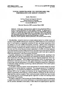
Fig. 1. Tuning of the controller (CP is the control plant, C is the controller, and RM is the reference model).
We note that the derivative x(n) is the highest derivative of the output variable for the nonlinear control object model (1). Although the differential equation for the control algorithm (3) contains x(n) , system (1) with the control algorithm (3) does not belong to the class of systems with control for the highest derivative [15 16]. This conclusion follows directly from expression (5), which is the result of the Laplace transform of the algorithm (3). In the control system discussed, it is recommended that the gain k0 is chosen from the condition k0 g(X, w) ≈ 1. In this case, the formation of the desired transient processes at the output of system (1) is reached by increasing the degree of separation of the rates between the fast and slow processes in the closed system, i.e., by reducing the parameter µ. From the expression for the characteristic polynomial of the FMS (9), it is evident that the requirement of accuracy in the formation of the desired transient processes at the output of system (1) is does not contradict the requirement of stability of fast processes since k0 g(X, w) ≈ 1. At the same time, this contradiction is the main drawback of systems with the control algorithm for the highest derivative [15, 16], where to improve the accuracy of formation of the desired transient processes at the output of system (1), it is required to increase the value of k0 g(X, w), which leads to a loss of stability of fast processes and, hence, to instability of the control system. CHOOSING PARAMETERS OF THE CONTROL ALGORITHM To simplify the tuning of the controller (3), as the parameters adn − 1 , . . . , ad1 and dq − 1 , . . . , d1 we choose the Newton binomial coefficients (s + 1)n = sn + adn − 1 sn − 1 + . . . + ad2 s2 + ad1 s + 1,
(11)
(s + 1)q = sq + dq − 1 sq − 1 + . . . + d2 s2 + d1 s + 1.
(12)
If we set k0 = 1/g(X, w), then it follows from the FMS (9) that the characteristic polynomial of the FMS is given by µq sq + dq − 1 µq − 1 sq − 1 + . . . + d1 µs + 1.
(13)
Based on expressions (4) and (13), the choice of the parameter µ can be made based on the ratio µ = T /η, where η is the desired degree of separation of the rates of fast and slow processes in the control system, for example, η ≥ 10. Correspondence between the behavior of the output of the plant (1) with controller (3) and the behavior of the reference model (10) can be determined from the diagram in Fig. 1a. TUNING OF THE CONTROLLER GAIN An advantage of the discussed tuning method is that for any values of q and n, where q ≥ n, the tuning of the controller (3) reduces to choosing the degree of separation of motions η and the gain k0 in such a manner that the requirement k0 ≈ 1/g(X, w) is satisfied at the working point. If the value of g(X, w) is unknown, tuning of k0 can be performed during direct identification of the high-frequency gain g(X, w), for OPTOELECTRONICS, INSTRUMENTATION AND DATA PROCESSING
Vol. 48
No. 5
2012
CALCULATION AND TUNING OF CONTROLLERS FOR NONLINEAR SYSTEMS
451
example, by introducing an auxiliary harmonic signal into the control channel. [17]. In this paper, we discuss a method of tuning the gain k0 by introducing an additional pulse signal u ¯ [18] into the control channel, as shown in Fig. 1b. Then, the equations of the closed system (1), (3) become x(n) = f (X, w) + g(X, w)[˜ u+u ¯]; (14) µq u ˜(q)
+ dq − 1
µq − 1 u ˜(q − 1)
+ . . . + d1
µ˜ u(1)
= k0
[F (X, r) − x(n) ].
System (14) leads to the equation of the FMS µq u ˜(q) + dq − 1 µq − 1 u ˜(q − 1) + . . . + d1 µ˜ u(1) + k0 g(X, w)˜ u = k0 [F (X, r) − f (X, w) − g(X, w)¯ u].
(15)
where g(X, w), F (X, r), and f (X, w) are considered as frozen quantities in the time interval of transient processes in the FMS (15). The influence of the pulse signal u ¯ on processes in the FMS depends on the transfer function G1 (s) = u(s)/¯ u(s), G2 (s) = u ˜(s)/¯ u(s). From (15) we obtain G1 (s) =
µq sq + dq − 1 µq − 1 sq − 1 + . . . + d1 µs ; µq sq + dq − 1 µq − 1 sq − 1 + . . . + d1 µs + k0 g (16)
G2 (s) = −
k0 g µq sq + dq − 1 µq − 1 sq − 1 + . . . + d1 µs + k0 g
.
If conditions (11), (12) are satisfied and k0 = 1/g(X, w), expressions (16) can be written as G1 (s) =
µq sq + dq − 1 µq − 1 sq − 1 + . . . + d1 µs ; (µs + 1)q (17) 1 G2 (s) = − . (µs + 1)q
Since the response of systems with the transfer functions (17) to the pulse signal u ¯ is known, the tuning of the gain k0 in a closed control system can be performed on the basis of a direct observation of the response of the signal u(t) and u ˜(t) to the pulse input u ¯(t). The change in the gain coefficient k0 ensures the admissible level of oscillations induced by the signal u ¯(t) in the FMS. The main criterion for the admissibility of the level of oscillations is the requirement of conservation of the conditions of separation of the rates between the fast and slow processes in the closed system, which is manifested in the fact that the time of decay of a pulsed transient induced by the control input should be negligibly small compared to the time of transient process for the output variable. Example. We consider the control plant model x ¨ = x3 + |x| ˙ − (2 + x2 )u + w.
(18)
In accordance with (6), we formulate the PID control law h 2 1 1 i µ2 u ¨ + 2µu˙ = k0 − x ¨ − x˙ − 2 x + 2 r . T T T
(19)
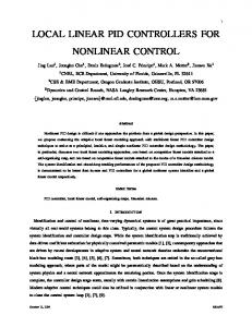
The results of numerical modeling of system (18), (19) are given in Figs. 2–5, where T = 0.3 s, µ = 0.03 s, and k0 = −0.5. Changing the gain k0 provides the admissible level of oscillations induced by the signal u ¯(t) in the FMS, as shown in Fig. 3, and simultaneously their correspondence to the type of response of the system with the transfer function G1 (s), presented in (17). The admissibility of the level of the induced pulse transient process for the control input u(t) in Fig. 3 is that the time of this process should be negligibly small compared to the time of the transient process for the output variable x(t) (see Fig. 2). OPTOELECTRONICS, INSTRUMENTATION AND DATA PROCESSING
Vol. 48
No. 5
2012
452
YURKEVICH 1.2
6
1.0
4
r(t)
2
x(t)
0.6
u(t)
r(t), x(t)
0.8
0.4
-2
0.2
-4
0 -0.2
0
0
2
4
6
8
-6
10 t, s
0
2
Fig. 2. Output of the control object.
6
8
10 t, s
8
10 t, s
1.0
2 1
0.5
0
u(t)
w(t)
4
Fig. 3. Control input.
0
-1 -0.5
-2 -3
0
2
4
6
8
10 t, s
-1.0
0
Fig. 4. External disturbance.
2
4
6
Fig. 5. Pulse input.
CONCLUSIONS The approach proposed in this paper provides a method for calculating and tuning standard PI or PID controllers, and, more generally, a universal controller for nonlinear dynamic systems of different types. It is shown that regardless of the orders of system (1) and controller (3), the tuning of the controller reduces to the choice of the degree of separation of motions η and the gain k0 . If g(X, w) is unknown, it is suggested that tuning of the coefficients k0 is performed by analysis of the response of the control input u(t) to an auxiliary pulse signal u ¯(t) in the control channel. This technique has been tested only by numerical simulations for various examples. There is no doubt that its application to the control of real technical objects, e.g., an inverted pendulum [19], is of great interest and is the subject of further research.
REFERENCES 1. V. Ya. Rotach, Automatic Control Theory: A Textbook for High Schools (MEI, Moscow, 2008) [in Russian]. 2. A. M. Shubladze and S. I. Kuznetsov, “Automatically Adjusted Industrial PI and PID Controllers,” Avtomatizatsiya v Promyshlennosti, No. 2, 15–17 (2007). 3. A. G. Aleksandrov and M. V. Palenov, “Self-Tuning PID/I Controller,” AIT, No. 10, 4–18 (2011). 4. K. J. Astrom and T. Hagglund, PID Controllers: Theory, Design, and Tuning. Research Triangle Park: Instrum. Soc. Amer., 1995. 5. A. O’Dwyer, Handbook of PI and PID Tuning Rules (Imperial College Press, London, 2003). 6. Y. Li, K. H. Ang, and G. C. Y. Chong, “PID Control System Analysis and Design,” IEEE Control Syst. Magazine 26 (1), 32–41 (2006). 7. V. D. Yurkevich, Synthesis of Nonlinear Nonstationary Control Systems with Different-Rate Processes (Nauka, St. Petersburg, 2000) [in Russian].
OPTOELECTRONICS, INSTRUMENTATION AND DATA PROCESSING
Vol. 48
No. 5
2012
CALCULATION AND TUNING OF CONTROLLERS FOR NONLINEAR SYSTEMS
453
8. V. D. Yurkevich, Design of Nonlinear Control Systems with the Highest Derivative in Feedback (World Scientific, 2004). 9. A. N. Tikhonov, “Systems of Differential Equations Containing Small Parameters at Derivatives,” Matematicheskii Sbornik 31 (3), 575–586 (1952). 10. E. I. Gerashchenko and S. M. Gerashchenko, Method of Motion Separation and Optimization of Nonlinear Systems (Nauka, Moscow, 1975) [in Russian]. 11. N. N. Krasovskii, “On the Stability of Solutions of a System of Two Differential Equations,” Prikl. Matematika Mekhanika 17 (6), 651–672 (1953). 12. D. S. Naidu, “Singular Perturbations and Time Scales in Control Theory and Applications: An Overview,” Dynamics of Continuous, Discrete and Impulsive Systems (DCDIS). Ser. B: Applications&Algorithms. 9 (2), 233–278 (2002). 13. P. D. Krut’ko, “Designing Algorithms for Controlling Nonlinear Plants Based on the Concept of Inverse Problems of Dynamics. Controlling Motion Relative to the Center of Mass,” Izv. Akad. Nauk SSSR. Ser. Tekhnicheskaya Kibernetika, No. 6, 129–138 (1986). 14. P. D. Krut’ko, Inverse Problems of Dynamics in Automatic Control Theory. Series of Lectures: A Handbook for Schools (Mashinostroenie, Moscow, 2004) [in Russian]. 15. A. S. Vostrikov, Synthesis of Control Systems by the Localization Method (Novosibirsk State Technical University, Novosibirsk, 2007) [in Russian]. 16. A. S. Vostrikov, “Controllers Synthesis for Automation Control Systems: State and Prospects,” Avtometriya 46 (2), 3–19 (2010) [Optoelectr., Instrum. Data Process. 46 (2), 107–120 (2010)]. 17. V. D. Yurkevich, “Adaptive Gain Tuning in Nonlinear Control Systems Designed Via Singular Perturbation Technique,” in: Proc. of the 18th Intern. Conf. on Control Applications Part of the 3rd IEEE Multi-Conference on Systems and Control, Saint Petersburg, Russia, July 8–10, 2009, 37–42. 18. V. D. Yurkevich, “PI/PID Control for Nonlinear Systems Via Singular Perturbation Technique,” Advances in PID Control. InTech, 2011, 113–142. 19. Yu. N. Zolotukhin and A. A. Nesterov, “Inverted Pendulum Control with Allowance for Energy Dissipation,” Avtometriya 46 (5), 3–10 (2010) [Optoelectr., Instrum. Data Process. 46 (5), 401–407 (2010)].
OPTOELECTRONICS, INSTRUMENTATION AND DATA PROCESSING
Vol. 48
No. 5
2012