Synthesis of Nonlinear Continuous Controllers for

Synthesis of Nonlinear Continuous Controllers for Verifiably-Correct High-Level, Reactive Behaviors Jonathan A. DeCastro and Hadas Kress-Gazit ∗ August 8, 2014

Abstract Planning robotic missions in environments shared by humans involves designing controllers that are reactive to the environment yet able to fulfill a complex high-level task. This paper introduces a new method for designing low-level controllers for nonlinear robotic platforms based on a discrete-state high-level controller encoding the behaviors of a reactive task specification. We build our method upon a new type of trajectory constraint which we introduce in this paper – reactive composition – to provide the guarantee that any high-level reactive behavior may be fulfilled at any moment during the continuous execution. We generate pre-computed motion controllers in a piecewise manner by adopting a sample-based synthesis method that associates a certificate of invariance with each controller in the sample set. As a demonstration of our approach, we simulate different robotic platforms executing complex tasks in a variety of environments.

1

Introduction

As robots become more sophisticated, we see increasing potential for them to perform complex tasks. Sensor-rich platforms such as self-driving cars, robotic manipulators, humanoids, and unmanned air vehicles enable capabilities ranging from human-assistance to search-and-rescue to exploration. To operate effectively in the real world, a robot must be able to perform tasks in a way that avoids causing harm to itself or the people it encounters, by appropriately reacting to the environment. Tasks that are reactive require that the robot’s behaviors change in response to realtime sensory information. It is therefore imperative that the controllers we provide to these robots produce behaviors that are guaranteed to satisfy all task instructions provided to the robot given our knowledge of the environment. Building upon existing concepts from the controller verification and motion planning communities, we present an automated methodology for computing (if possible) a set of verified controllers that fulfill the reactive behaviors of a high-level task. In the controller synthesis literature, recent activity has focused on solving the “reach-avoid” problem for nonlinear systems. Methods based on a game-theoretic representation of the problem have been solved [DGH+11], as have game-theoretic solutions involving a sequence of goals ∗ This work was supported by the NSF Expeditions in Computing project ExCAPE: Expeditions in Computer Augmented Program Engineering [grant number CCF-1138996]. The authors are with the Sibley School of Mechanical and Aerospace Engineering, Cornell University, Ithaca, NY 14853, USA, {jad455,hadaskg}@cornell.edu

1

[THDT12]. Rather than working directly with the nonlinear system, other researchers compute symbolic abstractions of the underlying system model [ZPMT12] for which efficient algorithms exist for the exact computation of reachable sets. The particular formulation in [ZPMT12] enables the synthesis of hybrid controllers for goal satisfaction with static obstacles [MDT10]. Concepts from nonlinear controller verification have been adopted in the motion planning domain. For example, libraries of verified motion plans have been generated for hybrid systems [JFA+07] as well as for nonlinear polynomial systems [TMTR10]. Both use a sampling-based strategy and employ solution methods that are efficient enough to allow on-line re-planning based on runtime sensor information [MTT12]. The latter method ( [TMTR10, MTT12]) builds upon the controller sequencing work of [BRK99] by combining sampling-based motion planning with local feedback controllers to define a robust neighborhood (funnels) computed about one of the sample trajectories. Controller sequencing has been applied to specific robotic applications; for example, in [CCR06], local verified motion controllers have been devised for robots with nonholonomic kinematic models. While each of these methods provide the framework for motion planning in the context of safety and reachability, they are not immediately equipped to handle automatic synthesis of controllers for reactive tasks with possibly infinite duration. Ongoing work in the robotics community has been devoted to developing provably correct synthesis algorithms for complex robot task specifications. A variety of techniques exist for synthesizing controllers for non-reactive tasks [KB06, LK04, Fra01, KF09, BKV10], as well as those for reactive tasks [WTM10, KGFP09]. The typical workflow is a three-step process: abstract the system model and the robot’s workspace; perform synthesis based on the abstraction and task specification; and design low-level controllers fulfilling each of the behaviors in the high-level controller. Low-level controller design can be performed using potential functions [CRC03], vector fields [BH04], or rapidly-exploring random trees (RRTs) [LaV06], to name a few. While such strategies often suffice for fully-actuated robots, correctness guarantees usually do not extend to robots with more complicated dynamics. The work of [KGCC+08] describes an application of provably-correct reactive synthesis to cars with a rear-drive Ackermann steering model. In that work, the authors manually designed a palette of controllers specific to the robot model that could be automatically instantiated in different environments. Here we describe algorithms for automatically generating such controllers for a wider class of nonlinear robot models. Some researchers have extended provably correct controller synthesis to nonlinear systems [LOTM13, WTM13]. These methods, however, rely on finding suitable discrete abstractions for the nonlinear system model, if any such abstractions exist. Others have introduced a multi-layered synthesis strategy in which the high-level controller is designed off-line, while the motion planning layer processes the high-level requests by accounting for nonlinear dynamics and any encountered workspace obstacles [BKV10, MLK+13]. However, the tasks that are considered in those works are non-reactive and the task fulfillment guarantees are obtained at runtime, rather than at the time of synthesis. Synthesis of provably-correct controllers for a complex vehicle in the presence of uncertainty is treated in [CB12]. The approach takes into account uncertainty bounds on the evolution of trajectories over time, however a challenge is in the application to reactive task specifications under indefinite execution durations. In the work of [FLP06], an automated framework is introduced for translating the behaviors of a high-level controller into low-level continuous controller specifications. The possibility exists to use such specifications in the design of nonlinear motion planners.

2

1.1

Problem Statement

In this paper, we address the following two questions. Given a high-level reactive mission plan (a control strategy consisting of deterministic region transitions that satisfy a user-defined mission specification), a robot model, and a workspace, can we design a set of low-level controllers that guarantee satisfaction of the task in a dynamic environment? If so, what is the set of allowable robot configurations for which these guarantees hold? To be precise, we are given a deterministic finite-state machine (FSM), the nonlinear differential equations of the robot, and a representation of the robot’s workspace. The FSM represents a control strategy synthesized from a high-level mission specification using, e.g., the approach described in [BJP+12]. The remaining problem - the focus of this paper - is devising a synthesis method that automatically generates a collection of low-level atomic controllers (if any exist) to realize each of the transitions in the FSM. In contrast to receding-horizon controllers (e.g. [WTM10, UMB13]) that are computationally expensive to implement on resource-constrained robots, the approach we adopt is based on a set of switched state-feedback controllers that are all precomputed offline. Thus, we aim for an efficient implementation at the expense of a slightly larger offline computational load compared to existing approaches. We work directly with coarsely-partitioned workspaces rather than synthesize controllers on a grid as in [LOTM13]. This is to alleviate the approximations needed to generate discrete abstractions and the complexity issues as workspaces are scaled larger. The main contributions of this work are as follows. First, building from the notion of sequential composition introduced in [BRK99, NP12], we define a new composition property, which we call reactive composition, to assure that the derived controllers produce continuous trajectories which guarantee the reactive behaviors of the FSM. That is, if the environment changes part-way through a transition, the robot must be able to correctly switch to a different transition. We do this by creating a set of constraints for the construction of low-level controllers. This part of the work is inspired by the general approach in [FLP06], however, in our work we extend controller specifications to encompass nonlinear robot models satisfying high-level reactive tasks. Another contribution of our work is an algorithm for synthesizing controllers that adhere to the reactive composition properties for the given task. The algorithm takes as an input a high-level controller with reactive behaviors, and tries to automatically synthesize a library of low-level (atomic) controllers that are guaranteed to satisfy these behaviors. To the authors’ knowledge, ours is the first attempt at designing verified controllers for reactive tasks. Finally, we contribute a sample-based method for computing controllers that implement each specific transition in the high-level controller, avoiding any unintended behaviors. We adapt the invariant funnels method in [TMTR10, MT12], which takes advantage of powerful numerical optimization techniques to produce a set of verifiably-safe atomic controllers. We introduce a new set of constraints in order to enforce reactive composition while preventing any robot behaviors prohibited by the high-level controller. In the authors’ preliminary version of this work, [DKG13], we introduced the concept of reactive composition, developed a constructive algorithm to ensure this property, and presented preliminary simulation results. This paper serves to build upon that work by detailing the precise technical conditions upon which reactively composable reachable sets should be constructed. Also, we explain the numerical method we use to compute atomic controllers, in particular our approach for incorporating the necessary invariance conditions for the reactive setting. We furthermore provide more illustrative examples in more complex environment settings. We motivate the work through an example.

3

R

C

3 (R) S blocked 2 (O)

S

4 (O)

1 (S)

O (a)

5 (C)

¬S blocked ¬S blocked ¬S blocked (b)

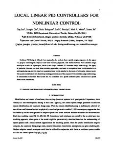
Figure 1: Workspace and FSM for Example 1. In (a), a 2-D environment is shown, along with a set of trajectories: one that does not satisfy the controller (solid) and one that does (dashed). The •’s indicate when S blocked turns from False to True. In (b), the number designates the state; the name in parenthesis denotes the region associated with that state. For each transition, the truth values for the S blocked sensor are given; unlabeled transitions imply that S blocked can take on any value. Example 1. Consider an autonomous delivery robot, modeled as fixed-wing aircraft, operating in a dense urban environment in Fig. 1a. The robot must continually deliver items between the store (S) and the restaurant (R) by visiting them infinitely often. If the plane is in O and en route to S but it senses that store is blocked, then it must re-route to the charging station C (without entering S). We adopt the synthesis approach in [BJP+12] to construct the FSM shown in Fig. 1b. Our goal is to construct feedback controllers that guarantee the sequence of motions of the FSM like the one in Fig. 1b using, in this case, a fixed wing airplane model and the workspace in Fig. 1a. This task is a reactive one because the behavior changes depending on whether or not the store is “blocked.” If the robot starts in S and S blocked stays False forever, the robot should follow the sequence of regions SOROS . . . indefinitely; if S blocked becomes True, then it may follow the sequence SOROCC . . ., i.e. the robot must go to C and stay there once it has visited R. In the continuous domain, there may be instances where the robot may fail this task. To see this, consider the solid-line trajectory pictured in Fig. 1a, where the plane moves counterclockwise starting with S blocked = False. If the robot senses S blocked = True at the •, it may be unable to avoid hitting S, and the task would fail. On the other hand, a clockwise trajectory (the dotted line in Fig. 1a), is likely to succeed in this workspace. In general, it is possible that S blocked may toggle between True and False at any point in the robot’s continuous trajectory, and so the robot must always be in a configuration where it can make any legal transition. If, for a different workspace, such controllers are found not to exist for the given platform, then the specified task may may not be suitable for that robot.

1.2

Paper Outline

In the next section, we introduce the reader to relevant background concepts for our atomic controller design approach. In Section 3, we introduce our approach to solving the problem and outline an algorithm for automatic controller synthesis. The trajectory-based approach used for computing verified controllers is presented in Section 4, and the execution of the controllers in Section 5. We then present simulations of tasks performed by different robots in Section 6. The

4

paper concludes in Section 7 with a summary and discussion.

2

Preliminaries

2.1

Robot and Environment Abstractions

Similar to the implementations in [KGFP09], we define an abstraction as a partitioning of the robot system and the environment in which it is operating. In particular, we partition the continuous map M ⊂ Rnw into M disjoint proposition-preserving map regions Mi , each associated with a label ri , where nw is the dimension of the workspace. In a planar environment, for example, the workspace is made up of two-dimensional polygons, some of which may represent holes in the map. We also assume that the robot can travel between any adjacent regions. In addition to the workspace, sensor and action values are discretized such that they may be effectively replaced by a set of Boolean propositions. Discretization is achieved by dividing the continuous space into a finite number of equivalence classes and assigning unique propositions to each class [KGFP09]. In this paper, we assume that sensors and actions are binary. Here sensors refer to events external to the robot (detection of a person, non-detection of a person), whereas actions refer to discrete robot functions (pick up, drop). We define X as a set of environment propositions, collecting sensor propositions, and Y as a set of system propositions, collecting robot action propositions and region propositions. Define the set R = ∪i ri ⊆ Y as the subset of Y corresponding to regions.

2.2

Controller Finite-State Machine

High-level controllers synthesized from task specifications and abstractions [WTM10,KGFP09] are assumed to be given in this work. The synthesized controller takes the form of a FSM A, defined as a tuple A = (X , Y, Q, Q0 , δ), where: • X and Y are proposition sets as defined in Section 2.1. • Q ⊂ N is a set of discrete states. • Q0 ⊆ Q is a set of initial states. • δ : Q × 2X → Q is a deterministic transition relation, mapping states and subset of environment propositions to successor states. We introduce the following additional definitions. Define γR : Q → R as a state labeling function assigning to each state the region label for that state, ri . Define the operator R : Q → Rn as a mapping that associates with each q ∈ Q the subset Xq = R(q) of the free configuration space X, where Xq corresponds to an n-D polytope labeled with γR (q). For example, a nonholonomic planar mobile robot with X ⊂ SE(2) would use 3-D polytopes for Xq ; Xq for higher-dimensional systems would be polytopes of appropriate dimension. We also define ∆ to be the collection of state-pairs corresponding to each transition, namely ∆ = {(q, q 0 ) ∈ Q2 | ∃z ∈ 2X . δ(q, z) = q 0 }. In this paper, we assume that actions other than locomotion are instantaneous. For some sequence w(0)w(1)w(2) . . ., w(i) ∈ 2X , i = 0, 1, 2, . . ., denote a run of A as q(0)q(1)q(2) . . ., with q(i + 1) = δ(q(i), w(i)). We call the sequence w(0)γR (q(0))w(1)γR (q(1)) . . . an execution trace of A. 5

2.3

Continuous Dynamics and Operations

In this paper, we consider systems of the form x˙ = f (x, u, d),

x(0) ∈ S,

d ∈ D,

u∈U

(1)

where we are given a state vector x ∈ X ⊆ Rn , a control vector u ∈ U ⊂ Rm , a vector of unknown disturbances d ∈ D ⊆ Rnd , and a set of initial states S. f is considered to be a smooth, continuous vector field with respect to its arguments. Under the action of a full-state feedback control law u(t) = κ(x(t), t), let x˙ = fˆ(x, d) represent the closed-loop system for (1) under κ(x(t), t). Given a concrete start state x(0) ∈ S and a time horizon T > 0 (a free parameter that will be discussed in Section 3.1), denote ξT : [0, T ] → X as a continuous finite-time trajectory of states under fˆ, µT : [0, T ] → U as a trajectory of control inputs, and ξTd : [0, T ] → D as a trajectory of disturbances. Say we are given a sequence of time indices, t ∈ {0, . . . , T }; then, we can represent the continuous trajectory as a sequence of states x = {ξ(τ )}τ ∈t , and a sequence of control inputs u = {µ(τ )}τ ∈t . Given a smooth function V (x, t), some ρ(t) > 0, and some T , we define the ρ-sub-level set as `(ρ(t), t) = {x | V (x, t) ≤ ρ(t)},

∀t ∈ [0, T ].

Let Xi , Xj ⊂ X be regions in the configuration space where Xi ∩ Xj 6= ∅ (the regions are adjacent). Define an atomic controller κij as a controller that steers f (x, u, d) from Xi to Xj without leaving Xi ∪ Xj under all possible disturbances. Formally, an atomic controller κij exists iff there exists some initial state ξT (0) ∈ Xi and some relative final time Tij such that ξT (Tij ) ∈ Xj and ξT (t) ∈ Xi ∪ Xj for all ξTd (t), t ∈ [0, Tij ]. We leave Tij as a free parameter to be chosen by the algorithm, as will be discussed subsequently. We refer to trajectories driven by the action of an atomic controller as atomic trajectories. Lastly, given Xi , Xj ⊂ X, define a reach tube Lij : [0, Tij ] → Xi ∪ Xj as the set of trajectories in which the controlled system remains for t ∈ [0, Tij ] under the action of a feedback controller. Formally, suppose that we define some initial set Sij and some atomic control law κij , then Lij = {ξT (t) | ξT (0) ∈ Sij , ∀ξTd (t), t ∈ [0, Tij ]}. We write Lij (t) to denote a slice of the reach tube Lij evaluated at time t. In the following, we abuse notation and write, for example, Xi ∪ Lij to express the union of Xi and the set covered by the reach tube (in place of Xi ∪k Lij (tk )).

3

Controller Synthesis Approach

To lay the foundation for our approach, in this section we introduce different classes of atomic controllers and the technical conditions that allow us to guarantee behaviors in the high-level controller. Lastly, we describe an algorithm which takes as its input the FSM and returns a library of atomic controllers that guarantee the continuous executions of the FSM at runtime.

3.1

Composition Strategies

i Define Iout = {k ∈ N | (qi , qk ) ∈ ∆} as the index set of all successor states for state qi (e.g. for 4 i state 4 in Fig. 1b, Iout = {1, 5}), and let Iout = {Iout }qi ∈Q . As defined by [BRK99], for a given set of atomic controllers to be sequentially composable, we require goal sets of the reach tubes to be contained within the domain of successor reach tubes. Formally:

6

(a)

(b)

Figure 2: Illustration of reactive composition. (a) shows a reach tube from R1 to R2 and possible trajectories. (b) shows a reach tube from R1 to R3 . Along any given trajectory leading to R2 (blue) in L12 ∩ L13 , there exist L13 trajectories (red dashed) leading to R3 also in L12 ∩ L13 . Definition 1 (Sequential Composition [BRK99]). Let Lij (t) denote the slice of Lij at time t. For Lij to j be sequential composable for each pair in ∆ implies that Lij (Tij ) ⊆ Ljk for all k ∈ Iout . For reactive tasks, the underlying conditions for sequential composition do not capture the possibility that the robot might need to change its motion part-way during a trajectory in response to some event. Consider again Example 1 and the two trajectories pictured in Fig. 1a. When the robot is in O with S blocked = False, and moving towards S, both trajectories may in fact satisfy the sequential composition property if atomic controllers exist for transitions between R and O and O and S. However, if S blocked turns True during the execution, the robot must already be in a state where it may access C without first entering S (a violation of the specification). The configurations where S is reachable from O must also be the set of configurations where C is reachable from O. We introduce a constraint called reactive composition to deal with co-reachability of successor regions. ¯ i ⊂ X denote the set of states such that, for all qi ∈ Q, there Definition 2 (Reactive Composition). Let X i ¯ i = ∩k∈I i Lik . A given reach tube Lij is reactively , i.e. X exists a trajectory from qi to any qk , k ∈ Iout out ¯i ∪ X ¯j . composable with respect to A if, for (qi , qj ) ∈ ∆, for all state trajectories ξT ∈ Lij ⇒ ξT ∈ X Reactive composability is illustrated in the 2-D scenario in Fig. 2b, where the solid blue trajectory shown exiting region R1 (corresponding to state 1) and entering R2 (state 2) is both contained completely within its own reach tube (shaded blue) and the reach tube (shaded red) for trajectories leading to R3 (state 3). Note that T12 and T13 signify the times beyond which all trajectories in L12 and L13 have reached their respective goal regions. As discussed next, we fulfill this property by imposing additional constraints on the reach tubes we generate.

3.2

Classes of Atomic Controllers

We now introduce two types of atomic controllers for constructing reactively composable controllers, and describe the constraints we apply in each case. Transition controllers κij refer to those which invoke a transition between adjacent regions. Inward-facing controllers κci are used to maximize coverage of the region. Respectively, the reach tubes for κij and κci are Lij and Lci .

7

3.2.1

Transition Reach Tubes, Lij

Consider a pair (qi , qj ) ∈ ∆. When we construct reach tubes for this transition, we want it to satisfy the current transition in the context of all possible subsequent transitions, that is, satisfy the reactive composition requirement. To this end, we introduce the following three conditions. ¯i ∪ X ¯ j : we want 1. Trajectories must be atomic with respect to the reactively composable set X trajectories to start in the set R(qi ) and progress to R(qj ) while remaining in an invariant ¯i ∪ X ¯j . Invij (defined in Section 3.2.2). For now, we apply definition 2 by choosing Invij = X 2. Trajectories must reach a goal set Gij ⊆ Xj ; formally, ξT (Tij ) ∈ Gij after some time Tij has elapsed relative to the start of the trajectory. We require Gij , whose precise definition will become clear in Section 3.2.2, in order for the reach tube to be sequentially composable with ¯j . reach tubes for successor states from qj . For now, we will assume Gij to be X 3. To prevent the robot from re-entering a region Xi once it has entered Xj for Xi 6= Xj , the trajectories need to be invariant in finite time to the set Xj . That is, for some τ ∈ [0, Tij ], ξT (τ ) ∈ ∂Xj ⇒ ξT (t) ∈ Xj , τ < t ≤ Tij where we denote ∂Xj to mean the boundary of the set Xj . To devise a certificate for the third condition, we can draw from region-of-attraction analysis [Kha02], as follows. Let V : Rn ×[0, Tij ] → R be a smooth differentiable function with V (ξT (t), t) = 0 and V (x, t) > 0, x 6= ξT (t). We further restrict V (x, t) to be bounded from below and above by class-K functions for all t ∈ R+ . [Kha02]1 We therefore want to ensure that the level set ∂`(ρ(t), t) = d V (x, t) < 0 on {x | x ∈ ∂`(ρ(t), t)∩Xj }. Put in terms of the {x | V (x, t) = ρ(t)} satisfies V˙ (x, t) = dt ˆ closed-loop system fij (·, ·), the third condition can be reduced to the easier problem of restricting ρ(t), the size of the attraction region, such that it satisfies: ∂ ∂ V (x = ξT (t), t) fˆij (ξT (t), d) + V (ξT (t), t) < 0, V˙ (x, t) = ∂x ∂t

ξT (t) ∈ ∂Xj ∪ `(ρ(t), t) 6= ∅, ∀d ∈ D.

Intuitively, this statement requires that the system flow toward the successor region only on that segment of the region boundary which is also in the computed region of attraction. We can satisfy these conditions by simultaneously imposing constraints on the construction of Lij (t). Respectively, these constraints are: Lij (0) ∩ Sij 6= ∅, Lij (t) ⊆ Invij ,

(2) ∀t ∈ [0, Tij ],

(3)

Lij (Tij ) ⊆ Gij , V˙ (x, t) < 0, ∀x ∈ Lij (t) ∩ ∂Xj 6= ∅,

(4) ∀d ∈ D,

∀t ∈ [0, Tij ].

(5)

where condition (2) assures that Lij has a nonempty intersection with the start set. Note that when ¯i. Xi = Xj , condition (5) can be dropped, and condition (3), the set inclusion Invij is merely X 1 In

Section 4, we will be choosing V (x, t) as a quadratic that satisfies these conditions.

8

3.2.2

Extending Controller Coverage: Inward-Facing Reach Tubes, Lci

Although in principle it is possible to employ transition controllers to synthesize atomic controllers for a given FSM, in practice, there are cases where it is impossible to find reactively composable sets which are not spatially disconnected, as required to satisfy (3). This can happen whenever the computed reach tubes are small compared with the region; for example, when constructing controllers in long corridors or regions with a large number of obstacles. In similar rationale to the techniques in [TMTR10, DRS11] that employ a maximization step to widen the basin of attraction to a goal region, we introduce another type of reach tube, inward-facing reach tubes, to achieve the needed spatial coverage. Consider a state qi ∈ Q. Our goal is to generate atomic controllers that admit finite-time trajectories and satisfy the following two conditions: 1. The region Xi must be invariant; that is, trajectories starting within some subset of Xi must remain in Xi . 2. Trajectories need to reach a goal set Gci ⊆ Xi ; that is, ξT (Ti ) ∈ Gci . The above statements require that trajectories are both invariant to the region and are sequentially composable with respect to Gci . This leads immediately to the following reach tube conditions: Lci (t) ⊆ Xi , Lci (Ti )

⊆

Gci .

∀t ∈ [0, Ti ],

(6) (7)

Notice that, by adding in the inward-facing controllers, we are able to expand the reactively¯ i ∪ Lc ) ∪ (X ¯ j ∪ Lc ), composable invariant in (3) (with a slight abuse of terminology) as Invij = (X i j c ¯ j ∪ L . As will be shown in the next and likewise also expand the goal set in (4) as Gij = X j section, this additional set of controllers will help our iterative approach for synthesizing atomic controllers. The larger the sets are, the greater the likelihood of finding controllers that satisfy the specification.

3.3

Atomic Controller Synthesis Algorithm

Using the composition strategies and the two types of atomic controllers, we now outline our process for constructing atomic controllers in Algorithm 1. The basic procedure is as follows. First, the set of all transitions ∆ are extracted from FSM A (AutomTransitions in line 1). Next, atomic controllers and their reach tubes are computed for each edge in ∆ in lines 7–17. Reach tubes are computed iteratively until either all possible configurations within R(qi ) for each qi are enclosed (to within a desired tolerance) or until it is determined that coverage is not possible, i.e. it is not possible to compute Lij for some (qi , qj ) ∈ ∆. The algorithm terminates successfully if reach tubes are found for each edge (line 20). If not, then the reach tube computations are revised by repeating lines 6–22 to ensure they are reactively composable in the sense of Definition 2. That is, each reach tube associated with either an incoming or outgoing transition from qi is checked whether or not it lies within the set of states for which all successor regions of qi are reachable.

9

Algorithm 1: (L, κ) ← ConstructControllers(A, R, f, , N ) Input: Synthesized FSM A with region mappings R(·), closed-loop robot dynamics f (·), coverage metric , and number of iterations N for coverage Output: A set of funnels L and controllers κ guaranteeing the execution of A 1 (∆, Iout ) ← AutomTransitions(A) 2 for (qi , qj ) ∈ ∆ do 3 Lij ← Rn 4 end c c 5 Li ← ∅, κi ← ∅ ∀qi ∈ Q 6 while True do 7 for (qi , qj ) ∈ ∆ do i Lik ∩ R(qi ) 8 Sij ← ∩k∈Iout   9 Gij ← ∩k∈I j Ljk ∩ R(qj ) ∪ Lcj out

10 11 12 13 14 15 16 17 18

19 20 21 22

(Lij , κij ) ← GetReachTube(Sij , Gij , Sij ∪ Lci ∪ Gij , f, , N ) if Lij = ∅ then return ∅ // No controller exists end i Sic ← R(qi )\ ∩k∈Iout Lik c i Gi ← ∩k∈Iout Lik ∩ R(qi ) (Lci , κci ) ← GetReachTube(Sic , Gci , R(qi ), f, , N ) end h   i

i if ∀(qi , qj ) ∈ ∆ : (Lij ∩ R(qi )) ⊆ ∩k∈Iout Lik ∩ R(qi ) ∪ Lci h   i (Lij ∩ R(qj )) ⊆ ∩k∈I j Ljk ∩ R(qj ) ∪ Lcj then out c c L ← (∪i,j Lij ∪i Li ), κ ← (∪i,j κij ∪i κi ) return L, κ end end

3.3.1

∧

Computing Lij

Fig. 3 illustrates, through an example, the computation steps in Algorithm 1. In the first iteration of lines 7–13, reach tubes are computed for each edge (qi , qj ) ∈ ∆. The set Lij is initialized as the whole configuration space, while the goal set Gij is the region R(qj ) and the invariant Invij is the region R(qi ) ∪ R(qj ). In Fig. 3a, reach tubes are computed for the two transitions (q1 , q2 ) (blue region) and (q1 , q3 ) (green region), and the intersection of the two is taken (yellow region). Intuitively, this intersection (see Fig. 3b) defines the set of states from which any region of successor states can be reached (by using either controller κ12 or κ13 ). The process repeats for the remaining edges in the FSM. The algorithm immediately returns failure if an edge is encountered where a reach tube cannot be constructed (lines 11–13).

10

(a)

(b)

(c)

(d)

(e)

(f)

Figure 3: Illustration of the reach tube computation steps, assuming symmetric transitions between each adjoining region. In (a), a pair of transition reach tubes L12 and L13 are computed for q1 , the intersection of which (yellow) defines the new start set for the next iteration (see lines 7–13 in Algorithm 1). In (b), the same is done for the remaining states q2 and q3 . Next, in (c), inward reach tubes Lci (red) are generated for each region, (see lines 14–17 in Algorithm 1). This expanded region defines the invariant for the next iteration. In (d)–(f), the process in lines 7–17 is again repeated for the new start sets and invariants, and terminates at (f) since all reach tubes lie inside the regions bounded by the dotted borders (e.g. for q1 this is R(q1 ) ∩ ((L12 ∩ L13 ) ∪ Lc1 )). 3.3.2

Computing Lci

In order to expand the size of reactively composable regions, we create inward reach tubes in lines 14–17 to provide controllers that steer the robot to a configuration from which it can take a transition. The collection of Lij from the current iteration produce the start sets Sic and the sequentially composable goal sets Gci for each qi . The set Sic in line 14 is the set R(qj ) minus the intersection of all transition reach tubes from that region (the white portions in Fig. 3b), while the set Gci in line 15 is found from Definition 1 (the yellow portions in Fig. 3b). In Fig. 3c, the red regions enclosed by the dashed lines, Lci , denote where controllers were found to drive the system into the yellow region. We seek transition reach tubes that are contained within the union of the red and yellow regions in Fig. 3c. 3.3.3

Further Iterations

After a single iteration, if the sequentially-composable transition reach tubes are not reactively composable, the algorithm continues alternately computing Lij and Lci until they are reactively composable for all Lij . To test if Lij is reactively composable, we need to determine if Lij is con11

tained within a subset of states where
outgoing
transitions from qi or qj are possible, i.e. satisfies c α Lαk ∩ R(qα ) ∪ L (Lij ∩ R(qα )) ⊆ ∩k∈Iout α for α ∈ {i, j}. As such, the termination criterion in line 18 enforces Definition 2, by requiring that transition reach tubes must either lie within an inward reach tube or the sets where any successor state is reachable. An additional iteration of the algorithm is shown pictorially in the bottom row of Fig. 3. In any given iteration, the sets Sij , Gij , and Invij for the ijth edge are updated by the Lij and Lci from the previous iteration. Fig. 3d shows the second iteration of lines 7–13, where new transition reach tubes for a are computed (L12 and L13 ), constrained to stay within the red and yellow regions for q1 , q2 , and q3 . After intersections are taken (yellow regions in Fig. 3e), the reach tubes from the previous iteration are replaced with a new set of inward reach tubes computed in lines 14–17. Fig. 3f illustrates this last step, and is an example of a situation where the algorithm successfully terminates because the reactive composability criterion in line 18 is fulfilled. If the algorithm terminates successfully, a library of reach tubes L is returned in lines 19–20 along with a library of controllers C.

4

Computing Atomic Controllers

We now present an implementation for constructing reach tubes in possibly cluttered workspaces. Probabilistic planning approaches, such as rapidly-exploring random trees [LaV06], have gained widespread use in various path planning applications. In such methods, exploration of the configuration space is probabilistically complete; that is, the probability of solving a motion planning problem for a given initial configuration improves with the number of samples. Recent techniques such as the Invariant Funnels technique in [TMTR10] uses sampled trajectories to compute verified controllers in a randomized tree structure. We adopt this framework to construct, in a piecewise manner, the reach tubes in Algorithm 1. For each computed sample trajectory, we also compute a region of invariance (funnel) about the sample trajectory. The workflow for constructing each funnel is as follows [TMTR10, MT12]: (1) generate a nominal trajectory connecting a given starting configuration and goal configuration, (2) design a local feedback controller to stabilize about the trajectory, and (3) solve a sum-of-squares program for the trajectory/controller pair to find the maximally-permissive funnel for this trajectory. Throughout this section, let us denote m as the index of a sample trajectory associated with some reach tube L. Let `m and κm denote, respectively, a funnel and controller associated with this trajectory. Each reach tube L is constructed from a collection of funnels such that L = ∪m `m . Likewise, each atomic controller κ is constructed from a collection of local controllers such that κ = ∪m κm .

4.1

Trajectory Generation

In our work, we solve a two-point planning problem to generate each sample trajectory, where we attempt to connect a point in S with a goal point in G. For differentially-flat platforms such as nonholonomic wheeled mobile robots, we apply feedback linearization [OLLV02]: a nonlinear transformation on the robot’s inputs yielding new pseudo-inputs that are derivatives of the robot’s Cartesian coordinates. For static feedback linearization the pseudo-inputs are upseudo = [x, ˙ y] ˙ T. We can then generate an instantaneous steering command by choosing this command to be the Cartesian vector displacement between the current robot configuration and the desired goal con-

12

figuration, i.e. upseudo = [x − xgoal , y − ygoal ]T . Using this strategy, we make use of standard ODE solvers to solve the planning problem. We discard those trajectories that do not satisfy the constraints for the current reach tube (as detailed in Section 3.2); those that are accepted are represented by the pair (ξTm , µm T ). For systems which are not feedback linearizable (e.g. 3-D Cartesian robot arms), trajectories can still be generated using nonlinear trajectory optimization methods [Bet09], or any number of motion planning tools.

4.2

Trajectory-Stabilizing Controllers

We apply local controllers to correct for deviations from the nominal sample trajectory due to disturbances or initialization errors. In this work, we use a linear quadratic regulator (LQR) approach [Kir76] applied to a linearized version of the system (1) based on the mth trajectory (ξTm , µm metric quantities x ¯(t) = x(t) − ξTm (t) and T ). LQR controllers are generated using the RT T m T u ¯(t) = u(t) − µT (t) using a cost function of the form 0 (¯ x Q1 x ¯+u ¯ Q2 u ¯)dt + x ¯T ST x ¯. The matrices Q1 , Q2 , and ST are design parameters that can be adjusted to tailor the shape of the funnels. In our case, we are interested in funnels with wide mouths (initial sets) and small tails (goal sets), so we typically choose ST one order of magnitude larger than Q2 , while the values in Q1 are chosen to remain within the same relative order as Q2 . The control gain K m (t) is computed based on the matrix solution S m (t) to a Riccati equation.

4.3

Invariant Funnels

m Given the nominal trajectory (ξTm , µm T ) and controller K (t), the task is to find a maximallypermissive funnel that satisfies the conditions in Section 3.2. The matrix solution to the Riccati equation from the controller generation step immediately parameterizes quadratic Lyapunov functions V m (x, t) = x ¯T S m (t)¯ x. Working with quadratic functions averts the problem of searching exhaustively over all classes of Lyapunov function candidates. Given that quadratic representations in general carry only local guarantees, the task is equivalent to finding a maximal ρm (t) such that the ρm (t)-sub-level sets of these Lyapunov functions `m (ρm (t), t) (represented as ellipsoids) satisfy the finite-time invariance conditions explained in [TMTR10], while also adhering to the conditions of Section 3.2. To explain our approach in the context of [TMTR10, MT12], we present the most general problem statement for solving for transition reach tubes using the system (1), then remark on which parts of the problem are changed when adapting the problem for inward-facing reach tubes. Computing a transition reach tube involves the following objective:

max ρm (t), s.t.

t ∈ [0, T m ]

(8)

ρm (t) ≥ 0, ∀t ∈ [0, T m ], V˙ m (x, t) ≤ ρ˙ m (t), ∀t ∈ [0, T m ], ∀x ∈ {x | V m (x, t) = ρm (t)}, ∀d ∈ D V˙ m (x, t) ≤ 0, m

m

m

m

m

∀t ∈ [0, T ], ∀x ∈ {x | V (x, t) = ρ (t)} ∩ Xj , m

m

` (ρ (t), t) = {x | V (x, t) ≤ ρ (t)} ⊆ Inv,

∀t ∈ [0, T ],

`m (ρm (T m ), T m ) = {x | V m (x, T m ) ≤ ρm (T m )} ⊆ G 13

m

(9) (10) (11) (12) (13)

where Xj is the polyhedral set corresponding to the successor state qj . Constraints (9) and (10) enforce trajectory invariance to the funnel and positive-semidefiniteness of the level set. The constraint (11) is a re-statement of (5) in the funnel setting. Likewise, (12) and (13) are, respectively, re-statements of the invariance (3) and goal (4) conditions. Condition (2) is not included here because satisfaction of the start set is implicitly satisfied by sampling the initial state of the trajectory from within S. It is worth pointing out that the difference between our formulation and the one in [MT12] is precisely the addition of conditions (11)–(13). Oftentimes, we find there are unknown disturbances (wind gusts pushing the robot in one direction or another), causing unexpected motions and collisions with obstacles. When we have such disturbances affecting the dynamics, we require that the invariance condition in (9) to be true for all d ∈ D. When computing funnels for inward reach tubes, the inequality (11) is removed and the inclusion (12) is replaced with the following: `m (ρm (t), t) = {x | V m (x, t) ≤ ρm (t)} ⊆ Xi to reflect the condition in (6). When solving the optimization problem in (8) – (13) using numerical methods, we replace the trajectory (ξT , κT ) with its discrete sequence (tm , κm , xm ). We then express the closed-loop system fˆ(x, d) under the action of κm as being polynomial in its arguments x and d. We then transform the problem (8)–(13) into a sum-of-squares program replacing the intervals [0, T m ] with tm and by making the following substitutions: Eq. (10) and (11):   ∂ m   − ∂x V (x, t)fˆ(t, x, 0) +    

Eq. (12):

Eq. (13):

∂ m ∂t V (x, t)

 + λ1 (x, t) (ρm − V m (x, t)) + λ2 (x, t)Pj (x) + λ3 (d, t)Pd (d) is s.o.s.,

t ∈ tm ,

λ1 (x, t), λ2 (x, t), λ3 (x, t) are s.o.s.,

t ∈ tm ,

  (V m (x, t) − ρm ) − λ (x, t)P (x) is s.o.s., t ∈ tm \ T m , 4 inv  λ4 (x, t) is s.o.s., t ∈ tm \ T m ,   (V m (x, T m ) − ρm ) − λ (x)P (x) is s.o.s., 5 G  λ5 (x) is s.o.s..

(14) (15)

(16)

Where λi (x, t), i = 1, . . . , 5 are positive-definite polynomial multipliers and Pj (x), Pinv (x),PG (x), and Pd (d) are all polynomials used in parameterizing the sets Xj , Inv, G, and D as zero-sub-level sets. In particular, Xj = {x | Pj (x) ≤ 0},

G = {x | PG (x) ≤ 0},

Inv = {x | Pinv (x) ≤ 0}, D = {d | Pd (d) ≤ 0}.

The sum-of-squares program is solved via the MATLAB toolboxes SPOT [Meg] and Ellipsoids [KV06].

14

4.4

Algorithm

The steps for generating reach tubes are encapsulated in an algorithm GetReachTube, outlined in Algorithm 2. The process is iterated up to N times. GetInit on line 4 randomly picks an initial point in the S. The function GetFinal on line 5 picks a final point inside G, seeking the centroid of the region if the goal set is a polygon and randomly if it is defined by reach tubes. With the boundary conditions defined, the algorithm next invokes SimTrajectory to generate a feasible trajectory and a controller based on the LQR design. Given a tm , the function returns a controller library κm as the sequence (µm , Km ), where µm = {µm (t)}t∈tm and Km = {K m (t)}t∈tm . A trajectory is deemed infeasible if it ever leaves the invariant for the current transition. If this happens, new final points and trajectories are generated until it is unobstructed. If a feasible trajectory is found, ComputeFunnels computes the funnels according to the procedure in Section 4.3. Lines 9–12 check if a feasible funnel is found. If so, it is appended to the existing library of funnels. Algorithm 2: (L, κ) ← GetReachTube(S, G, Inv, f, , N ) Input: A start set S, a goal set G, an invariant set Inv, along with f, , N Output: A set of reach tubes L and controllers κ 1 m ← 0, L ← ∅, κ ← ∅ 2 while V ol(L ∩ S) < (1 − )V ol(S) ∧ m < N do 3 m←m+1 4 xi ← GetInit(S) 5 xf ← GetFinal(G) 6 (tm , xm , κm ) ← SimTrajectory(f, xi , xf , Inv) 7 if xm 6= ∅ then 8 `m ← ComputeFunnel(tm , xm , cm , G, Inv) 9 if `m 6= ∅ then 10 L ← L ∪ `m 11 κ ← κ ∪ (tm , xm , κm ) 12 end 13 end 14 end 15 return L, κ Note that perfect coverage of a region is often not possible when the boundaries of a region are included as constraints. We allow for incomplete coverage by introducing a coverage metric  ∈ [0, 1] and declare the set covered if V ol(L ∩ S) ≥ (1 − )V ol(S) or if m = N where V ol is the volume of a particular set defined in Rn , m is the current funnel iterate, and N is an integer. Since the set S is represented as the intersections of unions of ellipsoids, the volume is computed in an approximate manner with the aid of the Ellipsoids toolbox [KV06]. The former condition asserts that coverage terminates if the volume of the reach tube L within the start set is a significant enough fraction of start set. If the coverage is not achieved before N iterations, then there may be transitions from region γR (qi ) that are not reachable from some parts of the state space R(qi ) for that region. Hence, the method is sound, but not complete. Another implementation issue arises from the curvature of the ellipsoidal level sets. At the 15

boundaries of polyhedral sets, coverage degenerates where the ellipsoid level sets meet the polyhedral region boundaries, sometimes causing difficulty when generating transition reach tubes. We work around this issue by relaxing the interface between neighboring regions by some fixed tolerance value reg . This parameter allows regions to share territory by an amount defined by this fixed distance. To more strictly enforce one of the two region boundaries, one can adjust the shared boundary in the direction of one region or another. Although not explored in this work, it is also possible to remove this shared boundary by altering our approach slightly to allow ellipsoidal level sets to be expanded beyond region boundaries as long as the boundary itself is certified as an invariant.

4.5

Complexity

Here we state the time complexity of our overall approach. The implementation in Algorithm 1 runs in time O(|Q|3 ). Put in terms of a set number of transitions |∆|, we can express this more precisely as O(|∆||Q|). Algorithm 2 applies two semidefinite programs; one for solving the sumsof-squares program and another for estimating the set volume. Both run in polynomial-time: the sums-of-squares solver is polynomial in both the state dimension n and the size of the FSM |Q|, while solver used for volume estimation is polynomial in n. In Section 6 we give more empirical insight into the complexity of the approach as a whole by providing actual runtimes when performing the computations for several example tasks.

5

Controller Execution

At runtime, low-level controllers are selected according to the current state of the robot and the current values of the sensor propositions. The planner executes the controller associated with the m funnel associated with the current robot state (e.g. κm ij if within `ij (t)). In order to adhere to the transitions of the controller FSM as the system evolves, a new funnel is selected if one of three events occur: (i) the end of a funnel is reached, (ii) a region transition is made and either an inward funnel or a transition funnel for the next transition is reached, or (iii) an environment proposition changes. Priority is always given to transition controllers κij over inward ones κci . That is, if the robot is currently executing a controller in κci and the trajectory reaches a funnel in Lij , with rj as the goal for that transition, the motion controller is switched from κci to κij . In Example 1, consider the case when the robot is in state q4 with S blocked = False. At the current time step, the robot is executing the controller κ34 and has just reached O. The next goal (S) is implemented by switching controllers to κ41 if within the associated funnel. Otherwise, the planner will choose κc4 . If the trajectory is in more than one funnel, the execution paradigm operates deterministically (the first funnel encountered in the library is always selected). We now show that the algorithm, when executed using the runtime implementation described above, produces trajectories that remain consistent with respect to the behaviors in the FSM. Define ω : R+ → X as a possible environment proposition trajectory initialized at ω(0). Let q(0) be the initial state, and ξ q(0) be a disturbance-free continuous trajectory in Xq(0) , with the robot’s configuration initially ξ q(0) (0). Let q(k), k > 0 be defined as follows. Initializing k = 0, τ0 = 0, we increment k either when a time t = τk > 0 is reached for which ξ q(k) (τk ) ∈ ∂Xq(k) (the trajectory reaches a boundary) or when δ(q(k), ω(τk )) = q(k) (a self-transition is already satisfied at time t = τk under the environment input ω(τk )). Each time k is incremented, let ξ q(k−1) (τk−1 ) = ξ q(k) (τk−1 )

16

to ensure continuity of the trajectories and build a trajectory segment ξ q(k) (t), t ∈ [τk−1 , τk ). To avoid livelock, we assume that the environment does not change too fast by restricting ω(t), t ∈ [τk , τk+1 ) to only those input traces for which livelocking does not occur for all k ∈ N. Given any such ω, we call the sequence σ = ω(0)R(q(0))ω(τ1 )R(q(1)) . . . a reactive execution trace associated with the continuous trajectory. In the following proposition, we show that the continuous trajectories obtained by executing the atomic controllers synthesized from Algorithm 1 yield reactive execution traces that enforce the behaviors of the high-level controller. i Proposition 1. Consider a robot initialized within ∩k∈Iout Lik ∪ Lci , qi ∈ Q0 ∧ (qi , ·) ∈ ∆. For all ω, executing Algorithm 1 produces a reactive execution trace σ of the high-level controller A.

Proof. To show that σ produced by the execution is in fact an execution trace of A, we remark that reach tubes are constructed from edges in ∆. For any (qi , qj ) ∈ ∆, the robot will either be in Lik i for some k ∈ Iout where conditions (3) and (4) hold true, or will be in Lci , where (6) and (7) hold true. Once in Xj , the robot will not re-enter Xi as a consequence of (5). Therefore, the robot will not exhibit additional behaviors not in A. To show that the converse is true; that is, there exists a σ for every possible execution path i of A, it is only necessary to show that, for any state in ∩k∈Iout Lik ∪ Lci , we can take any valid c i transition from qi . By construction, the set ∩k∈Iout Lik ∪ Li is reactively composable, thus proving completeness of the executions of A. Note that in general possible successor regions can be far away from each other and so, we cannot guarantee the behaviors of A for any arbitrary trajectory of environment propositions. For example, consider again state q4 in Example 1. The environment is allowed to toggle S blocked between True and False indefinitely when the robot is within O. In the continuous setting, this would cause the robot to get trapped forever in q4 , while in the FSM, there is no such livelock, since this toggling does not appear in the discrete execution. This is due to the physical setting in which robots operate and is a limitation of the abstraction, rather than the low-level controller synthesis approach.

6

Simulations

In this section, we demonstrate the application of the method developed in this paper to three examples. For these examples, we make use of a unicycle robot model consisting of three states, governed by the kinematic relationship: 

x˙ r





v cos θ



     y˙ r  =  v sin θ  ,     θ˙ ω where xr and yr are the Cartesian coordinates of the robot, θ is the orientation angle, and v and ω are, respectively, the forward and angular velocity inputs to the system. In this work, we augment

17

2 (r2 )

¬pursuer

pursuer

¬pursuer pursuer

1 (r1 )

3 (r3 )

4 (r2 )

(a)

(b)

Figure 4: (a) Workspace for the “patrolling two regions” example. (b) FSM for the example. The transitions are labeled with the truth value of the pursuer sensor; unlabeled transitions imply that pursuer can take on any value. the model by limiting ω such that

ω=

    ωmax

if u ≥ ωmax

if u ≤ ωmin

ωmin

  

u

otherwise

and v = vnom . The input u is governed by a feedback controller that steers the robot from some initial configuration to the desired configuration. We adopt the parameter settings ωmin = −3, ωmax = 3, and vnom = 2. For each example, we perform computations using MATLAB on a standard 64-bit Windows desktop machine, with an Intel Core i7 processor clocked at 3.40 GHz and 8 GB of RAM. To simplify our implementation, when computing funnels we make sure to choose from a single ρm regardless of the time index, so that ρ˙ m = 0.

6.1

Patrolling Two Regions

Consider a unicycle robot moving in the 10m × 9m workspace shown in Figure 4a. The robot is initially in r1 and must continually patrol r3 and r1 . If the robot senses a pursuer, then it must return to r1 (safe zone). The specification is implemented in the FSM shown in Figure 4b. A library of reactively-composable controllers is generated. For this example, we set the coverage metric  = 0.2, the number of iterations N = 100, and the interface relaxation reg = 0.2m. Reach tubes L23 are generated in the first and second iterations for (r2 , r3 ) and sample funnels are shown in Figs. 5 and 6. Also shown are the θ-slices of the union of the inward reach tube and transition reach tube Lc2 ∪ L21 (shown in red). In the first iteration, it is apparent that the funnel spans a gap in the set of inward funnels and hence the controllers are not reactively composable. If the controller drives the robot to this portion of the configuration space, the robot cannot change 18

(a)

(b)

Figure 5: (a) shows a transition funnel for the transition from r2 to r3 and a slice of the set where r1 is reachable from r2 at θ = 1.35 (defined by Lc2 ∪ L21 ) after the first iteration of Algorithm 1. (b) shows a 2-D view of the slice. In this iteration, the funnel is not reactively composable because the portion in r2 is not confined to the red set. If the robot is outside of the red set when enroute to r3 , there are no controllers which can deliver it to r1 if it sees a pursuer. direction if it senses a pursuer. We thus continue with another iteration of Algorithm 1. After the second iteration, the revised funnel is reactively composable for all transitions and no further iterations are necessary. The volumetric region coverage for each of the four states are shown in Table 1. Here, volume fraction is defined as the ratio of the actual volume of the region polytope i R(qi ) in (xr , yr , θ) and the subset of that polytope which contains ∩k∈Iout Lik ∪ Lci . Table 1: Fraction of (xr ,yr ,θ) coverage for each Xi associated with the FSM. q1

q2

q3

q4

(r1 )

(r2 )

(r3 )

(r2 )

0.5846

0.5976

0.5295

0.6171

Fig. 7a shows a sample trajectory of a robot starting in r1 , in which a controller in κ12 is applied, followed by a controller in κc2 and one in κ23 . Part way through its motion to r3 , the pursuer sensor turns True, invoking the sequence κc2 , κ21 to take the robot to r1 . pursuer once again becomes False prompting activation of a controller in κc2 followed by one in κ23 . As can be seen, the robot remains within the funnels and is able to satisfy the specification regardless of the environment as it moves between regions. Fig. 7b shows a long-term trajectory starting at a given initial condition in r1 ∩ ((L12 ∩ L11 ) ∪ Lc1 ). The figure indicates that the controllers generated by our algorithm can produce an infinite trajectory which is correct with respect to the infinite execution traces of A.

6.2

Pursuit-Evasion Game

Consider a game being played between a robot and an adversary, where the robot must repeatedly visit the home and goal regions pictured in Fig. 9, while evading an adversary which visits each of the three remaining regions infinitely often. Evasion is encoded by the requirement that the robot should never enter the same region as the enemy. By assuming the enemy patrols its three regions, 19

(a)

(b)

Figure 6: (a) shows a transition funnel for the transition from r2 to r3 and a slice of the set where r1 is reachable from r2 at θ = 1.05 (defined by Lc2 ∪ L21 ) after the second iteration of Algorithm 1. (b) shows a 2-D view of the slice. The funnel is now reactively composable because the portion of it which lies in r2 is now completely enclosed by the red set. The robot is therefore able to move to r1 if it senses a pursuer anywhere along its path to r3 .

(a)

(b)

Figure 7: Closed-loop trajectory generated from an initial state in r1 . (a) shows a set of control laws are applied to implement the transitions (r1 , r2 ) and (r2 , r3 ), driving the robot from state 1 to state 2, then from state 2 to state 3 in Fig. 4b. 2-D projections of the active funnels are also shown, the red corresponds to inward and green corresponds to transition. pursuer turns True when at the location marked by the “+” sign. At this instant, another controller is invoked to make the transition (r2 , r1 ). pursuer turns False at the “×” location, and new control laws are used to resume the transition (r2 , r3 ). (b) shows an long-term path when the robot starts at the red “” in r1 and pursuer remains False throughout.

20

Figure 8: FSM for the pursuit-evasion example. For simplicity, we label each edge by the value the sensor proposition must take, and exclude labels for which the remaining input labels can be inferred based on the assumptions on the enemy’s behavior. For example, the transition (q6 , q7 ) is labeled inR2; by mutual exclusion of the regions the enemy can occupy, when inR2 is True, inR1 and inR3 are False. the robot cannot get trapped forever in the goal region. As a fairness condition, in the specification we assume also that the enemy cannot enter the region the robot is currently in. The high-level controller (Fig. 8) consists of eight states and 13 transitions. The sensor values inR1, inR2 and inR3 correspond to the sensed location of the adversary. Reach tubes are constructed for each of the 13 transitions. A subset of these (the highlighted edges in Fig. 8) are shown in Fig. 9, showing the possible trajectories that the robot may follow when transitioning between goal and r3 (denoted green), and when transitioning between r3 and r1 . Note that the goal–r3 funnels all deliver the robot to the left of goal. The reason for this is that there are two possible transitions out of r3 (r1 and r2 ) depending on the location of the enemy. If the robot invokes these reach tubes, it always exits the left-hand facet of the goal region, where the robot is easily able to toggle between the goals r1 and r2 as the enemy toggles between those regions. The gray trajectory in Fig. 9 illustrates this for the case when inR1 remains True. Without reactive composition, a motion planner may cause the robot to exit goal via the top or bottom facets. If the robot follows the hypothetical magenta trajectory in Fig. 9, if inR1 stays True when in r3 , the robot will have no other option but to enter r1 (violating the specification) because there are neither any transition funnels L68 nor any inward funnels Lc6 in the area above the goal region.

6.3

Delivery in a Cluttered Environment

We next return to the example in Example 1. The task, once again, is to repeatedly deliver supplies between region S and R, connected via O, and return to C if the store S is blocked. We apply two models to fulfill this task: a model of the under-actuated unicycle and a model of a non-holonomic

21

Figure 9: Transition funnels for L56 and L67 (green) in the pursuit-evasion example. Lc5 and Lc7 are shaded blue and Lc6 is shaded red. Two hypothetical trajectories are shown; the one exiting the top of goal is not reactively composable and hence always enters r4 regardless of the environment when in r3 , while the one exiting the left face of goal is reactively composable allowing the robot to choose between entering r1 or r2 . car. The non-holonomic car is represented by the four-dimensional system:     x˙ r v cos θ      y˙   v sin θ   r     = ,  θ˙   v tan φ     `r  ω φ˙ where xr , yr , θ, v and ω are the same as for the unicycle, φ is the steering angle and `r is the axle spacing, which we take to be `r = 0.5 m. In this car model, we have control of both forward velocity v and steering rate ω, and impose no restrictions on their values. We apply Algorithm 1 to this problem for a workspace similar to the one shown in Figure 1a. Because the central region (O) consists of a large area interspersed with several obstacles, we forego attempting to cover the entirety of the region and instead seed inward controllers at configurations where transition controllers already reside. We do this to aid composition; for a given number of funnels, concentrating funnels together reduces gaps in the reactively- and sequentially-composable sets. Rather than keeping the goal region the same for all inward funnels, we attempt to increase coverage depth by permitting inward funnels to be sequentially composed with one another. We do this by redefining the goal region to include the most recent inward funnel each time one is computed. We limit the number of transition controllers to 20 and the number of inward controllers to 100. With these parameters, each major iteration in the while loop (lines 6–22) the MATLAB implementation took approximately 780 minutes to complete for the unicycle robot and 1470 minutes for the car. For both models, we terminate after two major loop iterations. We note that the method we introduce is intended as an offline verification and

22

controller synthesis approach, and therefore the code and computer hardware implementations were not optimized in this work. As constructed, the controllers are able to handle infinite executions of the high-level controller in Figure 1b. A partial sample trajectory for the unicycle robot starting in region S is shown in Figure 10. The controller coverage (projection of the inward and transition reach tubes onto xr , yr ) is indicated by the shaded regions in the map. In the first iteration of the synthesis algorithm, transition funnels initially cover a large portion of region O. After the first iteration, sampling of the funnel trajectories becomes more concentrated only in areas where reactive composition can be met. In our case, this is in the central part of the region. A side benefit to the approach is that the resulting controllers tend to yield efficient (non-circuitous) trajectories in the free configuration space. Figure 11 shows the same scenario as Figure 10, except using the car robot. Similar to the unicycle, the car robot is able to fulfill the transitions of the high-level controller. One of the differences is that the coverage area for the car is slightly smaller than the unicycle, which is primarily due to the dynamics being restricted by nonholonomic constraints. For both robot models, the trajectory remains within the verified reach tube for most of the trajectory, but in a few cases the trajectory momentarily exits the reach tube. This is attributable to the fact that we construct reach tubes based on an a polynomial approximation of the true dynamics. We simulate the polynomial approximation (dashed trajectories) in Figures 10 and 11. For both test cases, we have verified that the trajectories computed with the polynomial approximation do in fact remain within the funnels; this observation is reflected in the figures. If a bound on the divergence between the trajectories of the true system and its approximation can be found, we can use this bound to guarantee correctness in the actual system by imposing a certain amount of inflation on all obstacles and regions. We intend to address such approximation issues as future work.

Figure 10: Partial sample trajectories of the unicycle robot (solid), and its polynomial approximation (dashed) for the delivery scenario in Example 1 . The robot pose is shown at uniform time intervals, and the projection of the funnels appears as shaded fill areas. The red ◦ indicates the rising edge of the S blocked sensor. Note the yellow circled portion of the true system trajectory, indicating a place where it momentarily leaves the funnel.

23

Figure 11: Partial sample trajectories of the non-holonomic car (solid), and its polynomial approximation (dashed) for the delivery scenario in Example 1 . The robot pose is shown at uniform time intervals, and the projection of the funnels appears as shaded fill areas. The red ◦ indicates the rising edge of the S blocked sensor. Note the yellow circled portion of the true system trajectory, indicating a place where it momentarily leaves the funnel.

7

Conclusion

In this paper, a method is presented for synthesizing controllers in the continuous domain based on a discrete controller derived from a high-level reactive specification. The central contribution of this paper is an algorithm that generates controllers guaranteeing every possible execution of a finite-state machine for robots with nonlinear dynamics. Since a large number of computations are required to compute trajectories and funnels satisfying ellipsoidal constraints, the trade-off between completeness and complexity will need to be explored further. In contrast to the approach taken in this paper, one could devise a depthfirst strategy which seeks to generate atomic controllers in concentrated parts of the configuration space. While there is much to be gained in terms of computational efficiency (there would be fewer funnels in the database), this would be at the expense of completeness, since the vast majority of possible configurations would not be tied into the funnel libraries. If a set of atomic controllers cannot be synthesized, a natural question might be to ask: which parts of the specification, when modified, would allow the synthesis of controllers? If the algorithm fails to find a set of low-level controllers satisfying the specification, one may apply techniques such as the one in [GLB12] to revise specifications in such a way that low-level controllers exist. Creating a general, intuitive way of providing user feedback for specification revisions is a topic we intend to explore as future work.

Acknowledgment The authors are grateful to Russ Tedrake and Anirudha Majumdar for insightful discussions and advice with the technical implementations in this paper.

24

References [Bet09] John T. Betts. Practical Methods for Optimal Control and Estimation Using Nonlinear Programming. Cambridge University Press, New York, NY, USA, 2nd edition, 2009. [BH04] Calin Belta and L.C.G.J.M. Habets. Constructing decidable hybrid systems with velocity bounds. In Proc. of the 43rd IEEE Conf. on Decision and Control (CDC 2004), pages 467–472, Bahamas, 2004. [BJP+12] R. Bloem, B. Jobstmann, N. Piterman, A. Pnueli, and Y. Sa’ar. Synthesis of reactive (1) designs. Journal of Computer and System Sciences, 78(3):911–938, 2012. [BKV10] A. Bhatia, L.E. Kavraki, and M.Y. Vardi. Sampling-based motion planning with temporal goals. In IEEE International Conference on Robotics and Automation (ICRA 2010), pages 2689– 2696. IEEE, 2010. [BRK99] R.R. Burridge, A.A. Rizzi, and D.E. Koditschek. Sequential composition of dynamically dexterous robot behaviors. The International Journal of Robotics Research, 18:534–555, 1999. [CB12] Igor Cizelj and Calin Belta. Probabilistically safe control of noisy dubins vehicles. In Proc. of the IEEE/RSJ Int. Conf. on Intelligent Robots and Systems (IROS 2012), pages 2857–2862. IEEE, 2012. [CCR06] David C. Conner, Howie Choset, and Alfred A. Rizzi. Integrated planning and control for convex-bodied nonholonomic systems using local feedback control policies. In Robotics: Science and Systems, 2006. [CRC03] David C Conner, Alfred Rizzi, and Howie Choset. Composition of local potential functions for global robot control and navigation. In Proc. of 2003 IEEE/RSJ Int. Conf. on Intelligent Robots and Systems (IROS 2003), volume 4, pages 3546– 3551. IEEE, October 2003. [DGH+11] Jerry Ding, Jeremy Gillula, Haomiao Huang, Michael P. Vitus, Wei Zhang, and Claire J. Tomlin. Hybrid systems in robotics: Toward reachability-based controller design. IEEE Robotics & Automation Magazine, 18(3):33 – 43, Sept. 2011. [DKG13] Jonathan A. DeCastro and Hadas Kress-Gazit. Guaranteeing reactive high-level behaviors for robots with complex dynamics. In Proc. of the IEEE/RSJ Int. Conf. on Intelligent Robots and Systems (IROS 2013), 2013. [DRS11] Anca D. Dragan, Nathan D. Ratliff, and Siddhartha S. Srinivasa. Manipulation planning with goal sets using constrained trajectory optimization. In IEEE International Conference on Robotics and Automation (ICRA 2011), pages 4582–4588. IEEE, 2011. [FLP06] Georgios E. Fainekos, Savvas G. Loizou, and George J. Pappas. Translating temporal logic to controller specifications. In Proc. of the 45th IEEE Conf. on Decision and Control (CDC 2006), pages 899–904, 2006. [Fra01] Emilio Frazzoli. Robust hybrid control for autonomous vehicle motion planning. PhD thesis, Massachusetts Institute of Technology, 2001.

25

[GLB12] Ebru Aydin Gol, Mircea Lazar, and Calin Belta. Language-guided controller synthesis for discrete-time linear systems. In Thao Dang and Ian M. Mitchell, editors, Hybrid Systems: Computation and Control (HSCC’12), pages 95–104. ACM, 2012. [JFA+07] A. Agung Julius, Georgios E. Fainekos, Madhukar Anand, Insup Lee, and George J. Pappas. Robust test generation and coverage for hybrid systems. In Proc. of the 10th int. conf. on Hybrid systems: computation and control (HSCC’07), HSCC’07, pages 329–342, Berlin, Heidelberg, 2007. Springer-Verlag. [KB06] Marius Kloetzer and Calin Belta. A fully automated framework for control of linear systems from ltl specifications. In Proc. of the 9th Int. Conf. on Hybrid Systems: Computation and Control, HSCC’06, pages 333–347, Berlin, Heidelberg, 2006. Springer-Verlag. [KF09] S. Karaman and E. Frazzoli. Sampling-based motion planning with deterministic µcalculus specifications. In Proc. of the 48th IEEE Conf. on Decision and Control (CDC 2009), pages 2222–2229, 2009. [KGCC+08] Hadas Kress-Gazit, David C. Conner, Howie Choset, Alfred A. Rizzi, and George J. Pappas. Courteous cars. IEEE Robot. Automat. Mag., 15(1):30–38, 2008. [KGFP09] Hadas Kress-Gazit, Gerogios E. Fainekos, and George J. Pappas. Temporal logic based reactive mission and motion planning. IEEE Transactions on Robotics, 25(6):1370–1381, 2009. [Kha02] Hassan K. Khalil. Nonlinear Systems. Prentice Hall, 3rd edition, 2002. [Kir76] D.E. Kirk. Optimal Control Theory: An Introduction. Prentice-Hall, 1976. [KV06] Alex A. Kurzhanskiy and Pravin Varaiya. Ellipsoidal toolbox. Technical Report UCB/EECS-2006-46, EECS Department, University of California, Berkeley, May 2006. [LaV06] S. M. LaValle. Planning Algorithms. Cambridge University Press, Cambridge, U.K., 2006. Available at http://planning.cs.uiuc.edu/. [LK04] Savvas G. Loizou and Kostas J. Kyriakopoulos. Automatic synthesis of multiagent motion tasks based on ltl specifications. In Proc. of the 43rd IEEE Conf. on Decision and Control (CDC 2004), pages 153–158, 2004. [LOTM13] Jun Liu, Necmiye Ozay, Ufuk Topcu, and Richard M. Murray. Synthesis of reactive switching protocols from temporal logic specifications. IEEE Trans. Automat. Contr., 58(7):1771–1785, 2013. [MDT10] Manuel Mazo, Anna Davitian, and Paulo Tabuada. Pessoa: A tool for embedded controller synthesis. In 22nd International Conference on Computer Aided Verification (CAV 2010), pages 566–569, 2010. [Meg] A. Megretski. Systems http://web.mit.edu/ameg/www/.

polynomial

optimization

tools

(spot).

[MLK+13] MR Maly, M Lahijanian, Lydia E. Kavraki, H. Kress-Gazit, and Moshe Y. Vardi. Iterative temporal motion planning for hybrid systems in partially unknown environments. In ACM International Conference on Hybrid Systems: Computation and Control (HSCC), pages 353–362, Philadelphia, PA, USA, 08/04/2013 2013. ACM, ACM. 26

[MT12] Anirudha Majumdar and Russ Tedrake. Robust online motion planning with regions of finite time invariance. In Proc. of the Workshop on the Algorithmic Foundations of Robotics, 2012. [MTT12] Anirudha Majumdar, Mark Tobenkin, and Russ Tedrake. Algebraic verification for parameterized motion planning libraries. In Proc. of the 2012 American Control Conference (ACC), 2012. [NP12] Jerome Le Ny and George J. Pappas. Sequential composition of robust controller specifications. In IEEE International Conference on Robotics and Automation (ICRA 2012), pages 5190– 5195, 2012. [OLLV02] Giuseppe Oriolo, Alessandro De Luca, Ro De Luca, and Marilena Vendittelli. Wmr control via dynamic feedback linearization: Design, implementation, and experimental validation. Control Systems Technology, IEEE Transactions on, 10(6):835–852, November 2002. [THDT12] Ryo Takei, Haomiao Huang, Jerry Ding, and Claire J. Tomlin. Time-optimal multi-stage motion planning with guaranteed collision avoidance via an open-loop game formulation. In IEEE International Conference on Robotics and Automation (ICRA 2012), pages 323–329, 2012. [TMTR10] Russ Tedrake, Ian R. Manchester, Mark Tobenkin, and John W. Roberts. Lqr-trees: Feedback motion planning via sums-of-squares verification. I. J. Robotic Res., 29(8):1038–1052, 2010. [UMB13] Alphan Ulusoy, Michael Marrazzo, and Calin Belta. Receding horizon control in dynamic environments from temporal logic specifications. In Robotics: Science and Systems, 2013. [WTM10] Tichakorn Wongpiromsarn, Ufuk Topcu, and Richard M. Murray. Receding horizon control for temporal logic specifications. In Proc. of the 13th Int. Conf. on Hybrid Systems: Computation and Control (HSCC’10), 2010. [WTM13] Eric M. Wolff, Ufuk Topcu, and Richard M. Murray. Automaton-guided controller synthesis for nonlinear systems with temporal logic. In Proc. of the IEEE/RSJ Int. Conf. on Intelligent Robots and Systems (IROS 2013), 2013. [ZPMT12] Majid Zamani, Giordano Pola, Manuel Mazo, and Paulo Tabuada. Symbolic models for nonlinear control systems without stability assumptions. IEEE Trans. Automat. Contr., 57(7):1804–1809, 2012.

27