I n f o r m a t i o n T e c h n o lo g i e s , S y s t e m s A n a ly s i s a n d A d m i n i s t r a t i o n UDC 658.51.012
DOI: 10.29202/nvngu/2018-4/18
О. М. Pihnastyi1, Dr. Sc. (Tech.), Assoc. Prof., orcid.org/ 0000-0002-5424-9843, V. D. Khodusov2, Dr. Sc. (Phys.-Math.), Prof.
1 – National Technical University “Kharkiv Polytechnic Institute”, Kharkiv, Ukraine, e-mail:
[email protected] 2 – V. N. Karazin Kharkiv National University, Kharkiv, Ukraine
Calculation of the parameters of the composite conveyor line with a constant speed of movement of subjects of labour Purpose. The development of analytical methods for calculating the parameters of a composite conveyor line using the models containing partial differential equations. Methodology. To calculate the parameters of the conveyor line with a constant speed of movement of subjects of labour, the apparatus of mathematical physics is used. Findings. The solution is given in an analytic form that specifies the state parameters of the production line for a given technology position as a function of time. Originality. The scientific novelty of the results is the improvement of PDE-models of production systems of a conveyor type. The method for calculating the parameters of conveyor production, consisting of two connecting conveyor lines with a constant speed of movement of subjects of labour is offered. The considered method for calculation of conveyor production can be extended in case of a system with an arbitrary number of connecting conveyor lines. Practical value. The practical significance lies in the fact that the proposed method for calculating the parameters of conveyor production can be used to design control systems for conveyor production with an arbitrary number of conveyor lines. An essential advantage of this method is that each conveyor line is described by a single partial differential equation, the solution to which is obtained analytically. Such a representation makes it possible to use solutions for predicting the state parameters of a production line. Keywords: subject of labour, technological trajectories, technological process, conveyor, PDE-model, production cycle Introduction. At modern manufacturing enterprises with a flow-based method of production organization, the technological routes for manufacturing products contain 102‒103 technological operations [1], in the inter-operational reserves of which there are thousands of subjects of labour in unfinished production [2] (workin-process). Among the variety of models used for designing enterprise management systems with a streamlined method of production organization, four basic types are now clearly distinguished: discrete-event models (DES-model) [3], queuing models (QN-model), fluid models (Fluid-model) [4] and models using partial differential equations (PDE-model). The analysis of advantages and disadvantages of using each type of models is presented in [5]. It is shown that PDE-models, which are used to describe the production systems with a flow type of production organization, have a distinct advantage over other models in those cases when the production functions in a non-stationary mode. PDE-models are continuous models, the content of the partial differential equation, which allow taking into account the influence of the average speed of movement of labour subjects along the technological route on the macroscopic parameters of the production system: the duration of the production cycle, the amount of inter-operational reserves, the size of inter-operational accumulators, the rate of processing of subjects of labour. In this case, the models take into account the stochastic nature of the impact of technological equipment on the subject of labour during technological processing [6, 7]. The
concept of the minimum deviation of the enterprise output from existing demand and the concept of minimizing the supply of unfinished production are the main ones in designing the systems of production control. These production management concepts are implemented for production systems using PDE-models by regulating the input flow of raw materials F(t) and materials and the processing power of the subjects of labour [c]1y(t, S) at each technological operation [8]. It is assumed that the production system is ideal, that is, there is no loss of subjects of labour as a result of the production process (there are no defective products). The system of equations determining the behaviour of the parameters of the production line in a one-stage description has the following form [7, 9]
∂ c (t, S ) ∂ c (t, S ) 0 1 0; + = (1) ∂t ∂S
c (t, S ) = c (t, S ), (2) 1 1y under the initial condition
[c]0(t0, S ) = Y(S ), (3)
under the boundary condition
[c]0(t, S0) = F(S ),
(4)
© Pihnastyi О. М., Khodusov V. D., 2018
where [c]0(t, S ) is the density of the distribution of subjects of labour in unfinished production by technological positions; [c]1(t, S ) is the rate of processing of subjects of labour along technological positions at the time point . The position of the subject of labour in the technological route is characterized by a coordinate S [0; Sd] (Fig. 1).
138
ISSN 2071-2227, Naukovyi Visnyk NHU, 2018, № 4
I n f o r m a t i o n T e c h n o lo g i e s , S y s t e m s A n a ly s i s a n d A d m i n i s t r a t i o n When using the coordinates of the value space, the constant Sd corresponds to the cost of production. In a number of works, as a coordinate determining the position of the object, a dimensionless quantity x [0; 1] [9], the value of which gives an idea about the degree of processing of the subject of labour; x = 0 corresponds to the initial stage of processing the subjects of labour; x = 1 corresponds to the final stage of subjects of labour processing (the subject of labour turns into a finished product). The initial condition (3) determines the number of subjects of labour at a time point t0 at each technological operation. The solution to the system of equations (1–4) makes it possible to calculate the parameters of the production line without branching (Fig. 1). At the same time, most enterprises have technological processes, where the movement of labour subjects is carried out both sequentially and in parallel. The flow lines are a part of the technological routes that can be connected to each other and diverge [10]. The question of describing branched flow lines, even in the simplest form (Fig. 2), remains relevant. The analysis of the recent research and unsolved aspects of the problem of designing branched conveyor lines. The solution to the system of equations (1‒4) for a constant speed of movement of subjects of labour along the production line or along its individual part is presented in [11, 12]. However, a detailed analysis of the received solution is not given. At the same time, the calculation of the state parameters for conveyor lines is an important production task that requires the use of new methods of solution. Work [9] contains a numerical solution of the system of equations (1‒4) under specified initial and boundary conditions and the solution analysis is provided. The initial condition (3) determines the state of the subjects of labour at each technological operation at time point t = 0, and the boundary condition (4) spec-
ifies the intensity of the receipt of labour subjects for processing in accordance with existing orders for production. A numerical calculation of the production line consisting of three sections x [0, 0.2], x [0.2, 0.8], x [0.8, 1], is presented in [11]; at each of these sections the speed of the subject of labour g is constant and equals {15; 10; 15} respectively. Each of the sections represents a conveyor, providing a constant speed of movement of subjects of labour. The conveyors are placed one after another in succession. A special place is occupied by the problem of calculating the parameters of the state of the production system, consisting of several interconnected conveyor lines arranged both in series and in parallel [10]. An iterative algorithm [10], offered for planning a production system containing many branched technological routes, uses a deterministic discrete Fluid-model for describing the production system. It should be expected that using the class of PDE-models will allow obtaining a solution in a more compact form. Despite quite a large number of publications devoted to the design of control systems for production lines using PDE-models, the analysis of the conveyor line model has not received sufficient attention. It is especially necessary to single out the industrial systems with branched technological routes. At the same time, the conveyor type of production with branched technological routes is a widespread way of production process organization. The characteristic feature of this method of production organization is in the fact that all subjects of labour located on a specific conveyor line are moving at the same speed. The above-mentioned circumstance simplifies the system of equations (1–4). The purpose of this article is to construct an analytical solution to the system of equations (1‒4) for the case of movement of subjects of labour along the connecting
Fig. 1. The scheme of a single-station flow conveyor line
Fig. 2. The scheme of a two-station conveyor line ISSN 2071-2227, Naukovyi Visnyk NHU, 2018, № 4
139
I n f o r m a t i o n T e c h n o lo g i e s , S y s t e m s A n a ly s i s a n d A d m i n i s t r a t i o n technological routes with a conveyor way of organizing production for each of them. An important and specific task, along with the analysis of the obtained solution, is to demonstrate the dependence of the type of solution on the type of initial and boundary conditions that determine conveyor line functioning. The task of determining the state of the parameters of the conveyor line for an arbitrary moment of time, as well as the task of calculating the duration of the production cycle for manufacturing articles deserve attention as a result of solving the system of equations (1‒4). The production cycle of manufacturing products is one of the most important characteristics of the production system. Presentation of the main research. Let us consider the process of manufacturing products, which contains two technological routes of a conveyor type, united into one (Fig. 2). We choose the lower conveyor line as the main conveyor line, and the top line as an auxiliary conveyor line. The auxiliary conveyor line is used in a number of cases, one of which allows increasing the productivity of output for the main conveyor line. As a rule, the main line contains a critical route of product manufacturing. The subjects of labour with the (m-1) ‒ technological operation of the main line and the M-technological operation of the complementary auxiliary line get onto the m- technological operation of the main line. The system of equations describing the interaction of the joint lines has the form for the auxiliary production line
the subject of labour must correspond at the exit of the conveyor line in accordance with production and technological documentation. t0k, S0k – the moment of time and the coordinate of the technological position for which the initial or boundary conditions are determined, respectively. Parameters [ck]0(t, Sk) and [ck]1(t, Sk) are related to each other by a coefficient ak, that determines the conveyor line speed. For conveyors with the constant speed of movement ak = const. The righthand side of the equation (6d(S2 - S02)[c1](t, Sd1) is determined by the receipt of the subjects of labour for the technological position of the main line with the coordinate S2 = S02 from the auxiliary line to the main line with the rate [c1]1(t, Sd1) where δ(x) is the delta function ∞
∫ d ( S2 - S02 ) dS=2
-∞
We introduce dimensionless variables, by means of which we will describe the state of the parameters of the main line t = Td ⋅ t; Sk = Sdk ⋅ xk; k = 1, 2; c k (t, S k ) = qk (t, xk ) ⋅Q; Y k (S k ) = Q ⋅y k (xk ); 0 0 F k (t ) = Q ⋅ϑk (t), where Q = max{Y1(S1), F1(t)} + max{Y2(S2), F2(t)};
∂ c1 (t, S1 ) ∂ c1 (t, S1 ) 0 1 0; (5) + = ∂t ∂S1 [c1]1(t, S1) = a1[c2]0(t, S1),
under initial [c1]0(t01, S1) = Y1(S1),
gk =
∂ q2 (t, x2 ) 0
∂t
[c2]1(t, S2) = a2[c2]0(t, S2), (7) under initial [c2]0(t02, S2) = Y2(S2),
0
= (8)
[q2]0(t02, x2) = y2(x2); (9)
[q2]0(t, x02) = 2(t). (10)
The function [q1]0(t, 1) is unknown and is determined by solving the balance equation (5) for the auxiliary line that can be written down in a dimensionless form ∂ q1 (t, x1 ) 0
[c2]0(t, S02) = F2(t),
140
∂ q2 (t, x2 ) 0
or boundary conditions where Sk (0 ≤ Sk ≤ Ddk) are the coordinates of technological positions for the auxiliary (k = 1) and the main (k = 2) lines; [ck]0(t, Sk); [ck]1(t, Sk) is the value of interopretational reserves and the rate of processing of subjects of labour at a technological position that is characterized by the value Sk for the auxiliary (k = 1) and the main (k = 2) lines. The technological position with the coordinate Sk = Sdk corresponds to the degree of readiness of the subject of labour, that is, the state to which
+ g2
∂x2 = d ( x2 - x02 ) g1 q1 (t,1);
and for the leading production line ∂ c2 (t, S2 ) ∂ c2 (t, S2 ) 0 1 + = d ( S2 - S02 ) c1 (t, Sd1 ); (6) 1 ∂t ∂S2
ak ⋅Td 2 . Sd 2
Taking into account the introduced notations, we write the balance equation (6) for the main line in the dimensionless form
or boundary conditions [c1]0(t, S01) = F1(t),
1; S02 ∈ 0; Sd 2 .
∂t
+ g01
∂ q1 (t, x1 ) 0
∂x1
S g1 d 2 ; (11) = 0; g01 = S d1
[q1]0(t01, x1) = y1(x1); (12) [q1]0(t, x01) = 1(t).
(13)
The system of the following characteristics corresponds to a system of equations (11–13)
d x1 =g01; x1(t01 ) =x01; dt
(14)
ISSN 2071-2227, Naukovyi Visnyk NHU, 2018, № 4
I n f o r m a t i o n T e c h n o lo g i e s , S y s t e m s A n a ly s i s a n d A d m i n i s t r a t i o n d q1 dt
0
Taking (16‒18) into account, we can write down the expression [q1]0(t, 1) for a given initial condition
= 0; q1 (x1, t01 ) =y(x1 ). 0
[q1]0(t, 1) = y1(r01(1, t) + x01);
We integrate (14), we get
x1 = g01 ⋅ t + C1, C1 = const.
(15)
The function x1(t) can be interpreted as a position on the conveyor line of the τ, subject of labour at the time point t01 occupied the position x01. In this case, the conveyor belt movement is carried out with a constant dimensionless speed g01 (11). Equation (15), which determines the possible trajectories of the movement of subjects of labour in the phase coordinate space [12], is the first integral of equation (14). The general solution to equation (11) is the function of the first integral (15) [q1]0(t, x1) = [q1]0(x1 - g01 ⋅ t). Due to the fact that ∂ q1 (x1 - g01 ⋅ t) 0
∂t
= - g01
∂ q1 (x1 - g01 ⋅ t) 0
∂(x1 - g01 ⋅ t)
;
∂ q1 (x1 - g01 ⋅ t) ∂ q1 (x1 - g01 ⋅ t) 0 0 , = ∂x ∂(x1 - g01 ⋅ t) by direct substitution of the last expressions into equation (11) we obtain the equivalence - g01
∂ q1 (x1 - g01 ⋅ t) 0
∂(x1 - g01 ⋅ t)
+ g01
∂ q1 (x1 - g01 ⋅ t) 0
∂(x1 - g01 ⋅ t)
r01(1, t) = (1 - x01) - g01(t - t01), or if there is a boundary condition r (1, t) q1 (t,1) =ϑ1 t01 - 01 . 0 g01 If supplying subjects of labour at the initial moment of time t01 is carried out to the first technological position x01 = 0 of the free line, then condition (10) takes the form [q1]0(t, 0) = H(t - t01)1(t). We substitute [q1]0(t, 1) from the solution for the auxiliary conveyor line into the equation for the main conveyor line, we receive a closed system of equations. The state of the flow parameters of the leading conveyor line is determined by the state of the parameters of the auxiliary conveyor line. The system of characteristics corresponds to a system of equations (8–10) d x2 = g2 ; (19) dt
g2
d q2 (t, x2 )
= 0.
Taking into account the initial condition (12) and the boundary condition (13), the solution (11) has the form
0
d x2
Equation (19) allows us to obtain the first integral x2 - g2t = C2. (21)
We express t =
r q1 0 (t, x1 ) = q1 0 (x1 - g01 ⋅ t) = ϑ1 t01 - 1 , (17) g01
q2 0 (t, x2 )=
for the case when there is no discontinuity of the solution [q1]0(t, x1) the equality is done r y1(r1 + x01 ) = ϑ1 t01 - 1 , (18) g01
r1(x1, t01) = (x1 - x01); [q1]0(t, x01) = [q1]0(x01 - g01 ⋅ t) = 1(t); r1(x01, t) = -g(t - t0); y1(x01) = 1(t01), r1(x01, t01) = 0. ISSN 2071-2227, Naukovyi Visnyk NHU, 2018, № 4
x2
g
η - C2 ,1 d η= g2
∫ d ( η - x02 ) g12 q1 0 0
x - C2 g1 q1 2 ,1 + C3 , 0 g2 g2
we obtain a solution for the case if the initial condition (9)
(
)
q2 (t, x= H ( x2 - x02 ) - H ( x2 - x02 - g2 t ) × 2) 0 g r (x , t) × 1 q1 t20 - 2 2 ,1 + y 2 (r2 (x2 , t) + x02 ); 0 g2 g2
r1(x1, t) = (x1 - x01) - g01 ⋅ (t - t01).
[q1]0(t01, x1) = [q]0(x1 - gt01) = y(x1);
x2 - C 2 from (21) and insert it in (20) g2
= H ( x2 - x02 )
where the variable is introduced The substitution of t = t01 in (27) and x = x01 in (17) gives the identical equalities to the initial and boundary conditions
0
[q2]0(t02, x2) = y2(x2).
[q1]0(t, x1) = [q1]0(x1 - g01 ⋅ t) = y1(r1 + x01), (16) or
= d ( x2 - x02 ) g1 q1 (t,1); (20)
r2(x2, t) = (x2 - x02) - g2(t - t02), (22)
and the solution for the case if the initial condition (10) is given g r (x , t) q2 (t, x2= ) H ( x2 - x02 ) 1 q1 t20 - 2 2 ,1 + 0 0 g2 g2 r2 (x2 , t) +ϑ2 t20 . g2 141
I n f o r m a t i o n T e c h n o lo g i e s , S y s t e m s A n a ly s i s a n d A d m i n i s t r a t i o n The solution [q2]0(t, x2) (22) for the function [q1]0(t, 0) = 1(t) = 1; [q1]0(0, x1) = y1(x1) = 0; (23) 1 q2 (0, x2 ) = y 2 (x2 ) = ( 2 + sin(2πx2 ) ), (24) 0 3
with the source of receiving subjects of labour on the main line at the point x02 = 0, is shown in Fig. 3. The rate of receipt of the subjects of labour for the first technological operation is determined by the expression λ(t= = ) g2 q2 (t,0) 0
g2 ( 2 - sin(2πg2 t)), (25) 3
with the initial distribution of subjects of labor along the technological operations of the conveyor line [q2]0(0, x2) = y2(x2) at the time point t = 0. The combination of the conveyor lines is carried out in the technological position with the coordinate x2 = 0.2. The arrival of subjects of labour from the auxiliary line onto the technological position x2 = 0.2 of the main line begins at the time point τ = 0.2, which is determined by solving the system of equations (8–15). The distribution of subjects of labour [q2]0(t, x2) along the technological positions of the conveyor for time points t = (t/Td) = {0.0; 0.1; 0.2; …; 0.9; 1.0} separately is shown in Fig. 4. Conditions (23) for the auxiliary conveyor line indicate that at the initial time point t = 0 the auxiliary conveyor line was empty. At point of time t = 0 the first technological position receives the subjects of labour with intensity g011(t). The distribution of labour subjects at time points τ = = 0.1, τ = 0.2 is determined by the displacement of the initial distribution of labour subjects along the conveyor line with the dimensionless speed g1. At time point τ = = 0.2, the first subject of labour on the auxiliary line underwent technological processing at the last technological operation. The technological position of the main conveyor line with the coordinate x2 = 0.2 received the r (x , t) subjects of labour with intensity g1 q1 0 t20 - 2 2 ,1 . g2 The source of additional receipt of subjects of labour [q2]0(t, x2) forms a jump at the technological position x2 = 0.2 at time point τ > 0.2 with the height
g g q1 (t,1) 1 =ϑ1 ( t ) 1 . In the case considered, where 0 g g 2
2
g 1. The total numg1 = g2 the jump equals q1 0 (t,1) 1 = g 2
ber of subjects of labour from the main and auxiliary production lines moves with the dimensionless speed of the conveyor line g1 along the technological route (Fig. 3), t = {0.3; 0.4; 0.5; …; 0.9}. The change in the number of subjects of labour in time in the inter-operational reserves of the technological positions of the main conveyor line, determined by the coordinate x2 = (S/Sd) = = {0.0; 0.1; 0.2; …; 0.9; 1.0;} is presented in Fig. 5. Starting from the point of time τ > 0.2, the influence of work of the auxiliary conveyor line is seen at the technological positions of the main conveyor line. The function jump [q2]0(t, x2) for the technological position x2 = 0.2 at the time point τ = 0.2 2 is spread with the speed of the conveyor movement g2 to subsequent technological operations. The state of technological reserves for technological positions, characterized by dimensionless coordinates x = (S/Sd) = {0.0; 0.1; 0.2; …; 0.9;}, is shown in Fig. 6. The spread of a jump-like increase in the state of inter-operational production stocks in time is clearly shown. Let us determine the rate receipt of subjects of labour onto the first technological position of the main line. The distribution of labour subjects along the technological positions with the initial condition (23) creates a source for the first technological position, ensuring the receipt subjects of the labour at a rate determined by the solution [q2]0(t, x2). The change of the value of inter-operational reserves for the first technological operation with the given rate of receipt at the first technological position (25) is presented in Fig. 6 for x2 = (S/Sd) = 0. The characteristic equation (19) determines the trajectories of movement of individual subjects of labour (21) along the technological route along the main conveyor line. As expected, the movement of an individual object of labour along the trajectory (21) is carried out at a constant speed equal to the speed of the conveyor line. Equation (19) makes it possible to calculate the duration of the production cycle of product manufacturing (Fig. 7). The duration of the production cycle is equal to the time interval during which the subject of labour
Fig. 3. The distribution of subjects of labour [q2]0(t, x2) along the technological positions of the conveyor for moments of time t = (t/Td) = {0.0; 0.1; 0.2, …; 0.9; 1.0}, where g2 = g1 = 1.0; Sd2 = 0.2Sd1 142
ISSN 2071-2227, Naukovyi Visnyk NHU, 2018, № 4
I n f o r m a t i o n T e c h n o lo g i e s , S y s t e m s A n a ly s i s a n d A d m i n i s t r a t i o n
a
b
c
d
e
f
g
h
i
j
Fig. 4. The distribution of subjects of labour [q2]0(t, x2) along the technological positions of the conveyor for time points t = (t/Td) = {0.0; 0.1; 0.2; …; 0.9}, where g2 = g1 = 1.0; Sd2 = 0.2Sd1: a ‒ τ = 0.0; b ‒ τ = 0.1; c ‒ τ = 0.2; d ‒ τ = 0.3; e ‒ τ = 0.4; f ‒ τ = 0.5; g ‒ τ = 0.6; h ‒ τ = 0.7; i ‒ τ = 0.8; j ‒ τ = 0.9
Fig. 5. The dependence of the quantity of the subjects of labour at the technological position of the conveyor on time at g2 = = g1 = 1.0; Sd2 = 0.2Sd1 for the values of coordinate x = (S/Sd) = {0.0; 0.1; 0.2; …; 0.9; 1.0;} ISSN 2071-2227, Naukovyi Visnyk NHU, 2018, № 4
143
I n f o r m a t i o n T e c h n o lo g i e s , S y s t e m s A n a ly s i s a n d A d m i n i s t r a t i o n
a
b
c
d
e
f
g
h
i
j
Fig. 6. The dependence of the quantity of subjects of labour [q2]0(t, x2) at the technological position of the conveyor on time for the values of coordinate x = (S/Sd) = {0.0; 0.1; 0.2; …; 0.9;}, when g2 = g1 = 1.0; Sd2 = 0.2Sd1:
a ‒ x2 = 0.0; b ‒ x2 = 0.1; c ‒ x2 = 0.2; d ‒ x2 = 0.3; e ‒ x2 = 0.4; f ‒ x2 = 0.5; g ‒ x2 = 0.6; h ‒ x2 = 0.7; i ‒ x2 = 0.8; j ‒ x2 = = 0.9
Fig. 7. Set of characteristics x = gt + C; C = {0.2; 0.1; 0.0; …; -0.7; -0.8;}; g2 = g1 = 1.0; Sd2 = 0.2Sd1 passes from the first technological position to the last. The calculation of the production cycle for enterprises
using the simplified method of production organisation is given in [12]. The value of duration of the production
144
ISSN 2071-2227, Naukovyi Visnyk NHU, 2018, № 4
I n f o r m a t i o n T e c h n o lo g i e s , S y s t e m s A n a ly s i s a n d A d m i n i s t r a t i o n cycle for a conveyor-type production line can be determined as follows = td
1
dx
∫= g2 0
1
1 1 = dx . g2 ∫0 g2
It should be pointed out that the results of the work are of scientific and practical interest for designing the speed control systems for conveyor belt systems, which found widespread use in mining industry [13‒15]. An important result of this work is also the method for calculating the duration of the production cycle, based on the use of characteristic equation (19). This method makes it possible to construct the dependence of the length of production from the distribution of labour subjects along the conveyor line at the moment of time, which determines the arrival of the first subject of labour for processing at the first technological operation. Thus, the duration of the production cycle is not a constant value; it is determined by the load for operating production. A further perspective for the development of the issue discussed in this paper is the construction of a conveyor line control system and the extension of the offered method for calculating conveyor lines for the system “main line ‒ N-auxiliary lines”.
The products put onto the conveyor line at a dimensionless point of time t1, exit as a finished product at a time point t2 with a backlog td = (t2 - t1), which equals the time of the production cycle. Backlog (t2 - t1) does not depend on the time point of receiving the order for production, it is a constant value, inversely proportional to the dimensionless speed of the conveyor line td =g2-1. The state of the flow line parameters at the exit is determined by the state of the production line at the input with a backlog on a constant value. Conclusions and further prospects for the development and improvement of PDE-models of production systems. The received results of the research are fundamental for the development of control systems for production of a conveyor type, consisting of the main and a number of auxiliary lines. The dependence of the state of the interoperational reserves of the main conveyor line on the state of the inter-operational reserves of auxiliary conveyor line is shown. The influence of initial and boundary conditions of the auxiliary line on the state parameters of the main conveyor line is considered. Except for the case considered in the present article, the boundary condition (4) can be claimed in the case when the model of the production line takes into account the offloading of the subjects of labour in the form of a semi-finished product from the technological position characterized by coordinate or the presence of the factors which determine accounting of the amount of defective products in the model. The presence of initial (3) and boundary (4) conditions leads to the interrupted character of the solution of the system of equations, which is characteristic for the behaviour of the flow parameters of modern production conveyor lines [1‒4]. The model of the production system of a conveyor type, in which auxiliary lines are used as the subjects of management for ensuring the required output of finished products by the enterprise, is of interest. The main line operates in a continuous mode, while auxiliary conveyor lines in the on/off mode, which allows regulating the output of finished products. It should also be pointed out that, unlike the liquid models, the PDE model uses one equation for one non-branched route, and not for each piece of equipment included into the technological route. So, for example, to describe the production system [1], containing 102‒103 technological operations, using the liquid model it would be necessary to solve 102–103 differential equations describing the operation of individual production units. Along with the advantages in describing complex production systems of the flow type, the use of PDEmodels is bound by a number of difficulties, one of which is the construction of a closed system of equations for the production process. In the present paper, the derivation of a closed system of equations is solved by using an additional equation determining the conveyor speed, which allows us to derive equation (2).
References. 1. Armbruster, D., Ringhofer, C. and Jo, T-J., 2004. Continuous models for production flows. In: Proceedings of the 2004 American Control Conference. Boston, MA, USA, 2004, pp. 4589–4594. DOI: 10.23919/ACC.2004.1384034. 2. Schmitz, J. P., van Beek, D. A. and Rooda, J. E., 2002. Chaos in Discrete Production Systems. Journal of Manufacturing Systems, 21(3), pp. 236–246. DOI: 10.1016/S0278-6125(02)80164-9. 3. Law, A. M., 2015. Simulation Modeling and Analysis. McGraw-Hill. 4. Grosler, A., Thun, J. H. and Milling, P. M., 2008. System dynamics as a structural theory in operations management. Production and operations management, 17(3), pp. 373‒384. DOI: 10.3401/poms.1080.0023. 5. Pihnastyi, O. M., 2014. On a new class of dynamic models of conveyor lines of production systems. Nauchnye vedomosti Belgorodsko-go gosudarstvennogo universiteta, 31/1, pp. 147‒157. Available at: [Accessed 5 October 2017]. 6. Armbruster, D., Marthaler, D. and Ringhofer, C., 2006. Kinetic and fluid model hierarchies for supply chains supporting policy attributes. Bulletin of the Institute of Mathematics. Academica Sinica, pp. 496–521. Available at: [Accessed 11 September 2017]. 7. Demutskii, V. P., Pihnastaia, V. S. and Pihnastyi, O. M. 2005. Stochastic description of economic-indudtrial systems with large turnout. In: Dopovіdі Nacіonal›noї akademії nauk Ukraїni. Kiev: Vidavnichij dіm Akademperіodika, 7, pp. 66–71. Available at: [Accessed 14 September 2017]. 8. Lefeber, E., Berg, R. A. and Rooda, J. E., 2004. Modeling, Validation and Control of Manufacturing Systems. In: Proceeding of the 2004 American Control Conference, Massachusetts, 2004, pp. 4583–4588. DOI: 10.23919/ACC.2004.1384033. 9. Armbruster, D. A., Marthaler, D., Ringhofer, C., Kempf, K. and Jo, T-C., 2006. Continuum Model for a Re-entrant Factory. Operations research, 54(5), pp. 933–950. DOI: 10.1287/opre.1060.0321.
ISSN 2071-2227, Naukovyi Visnyk NHU, 2018, № 4
145
I n f o r m a t i o n T e c h n o lo g i e s , S y s t e m s A n a ly s i s a n d A d m i n i s t r a t i o n 10. Tian, F., Willems, S. P. and Kempf, K. G., 2011. An iterative approach to item-level tactical production and inventory planning. International Journal of Production Economics, 133, pp. 439–450. DOI: 10.1016/j.ijpe.2010.07.011. 11. Armbruster, D., Degond, P. and Ringhofer, C., 2006. A model for the dynamics of large queuing networks and supply chains. SIAM Journal on Applied Mathematics, 83, pp. 896–920. DOI: 10.1137/040604625. 12. Demutskii, V. P., Pihnastaia, V. S. and Pihnastyi, O. M., 2003. Enterprise theory: Stability of mass production functioning and promoting products into the market. Har’kov.: HNU, 272 p. DOI: 10.13140/RG.2.1.5018.7123. 13. Halepoto, I. A., Degond, P. and Ringhofer, C., 2016. Design and Implementation of Intelligent Energy Efficient Conveyor System Based on Variable Speed Drive Model. Control and Physical Modeling International Journal of Control and Automation, 9(6), pp. 379‒388. DOI: 10.14257/ijca.2016.9.6.36. 14. Hiltermann, J., Lodewijks, G., Schott, D. L., Rij senbrij, J. C., Dekkers, J. and Pang, Y., 2011. A methodology to predict power savings of troughed belt conveyors by speed control. Particulate science and technology, 29(1), pp. 14–27. DOI: 10.1080/02726351.2010.491105. 15. Lauhoff, H., 2005. Speed Control on Belt Conveyors – Does it Really Save Energy? Bulk Solids Handling Publ., 25(6), pp. 368‒377. Available at: [Accessed 14 May 2017].
Розрахунок параметрів складеної конвеєрної лінії з постійною швидкістю руху предметів праці О. М. Пiгнастий1, В. Д. Ходусов2 1 – Національний технічний університет „Харківський політехнічний інститут“, м. Харків, Україна, e-mail:
[email protected] 2 – Харківський національний університет імені В. Н. Ка разіна, м. Харків, Україна
Мета. Розробка аналітичних методів розрахунку параметрів складеної конвеєрної лінії з використанням моделей, що містять рівняння у приватних похідних. Методика. Для розрахунку параметрів конвеєрної лінії з постійною швидкістю руху предметів праці використано апарат математичної фізики. Результати. Рішення дано в аналітичному вигляді, що визначає стан параметрів потокової лінії для заданої технологічної позиції як функцію часу. Наукова новизна. Полягає в удосконаленні PDE-мо делей виробничих систем конвеєрного типу. Запропоновано метод розрахунку параметрів конвеєрного виробництва, що складається із двох конвеєрних ліній, що з’єднуються з постійною швидкістю руху предметів праці. Розглянутий метод розрахунку конвеєрного виробництва може бути поширений на випадок системи з будь-якою кількістю конвеєрних ліній, що з’єднуються. Практична значимість. Полягає в тому, що запропонований метод розрахунку параметрів конвеєрного виробництва може бути використаний для 146
проектування систем управління з будь-якою кількістю конвеєрних ліній. Істотною перевагою методу є те, що кожна конвеєрна лінія описується одним рівнянням у приватних похідних, рішення якого отримано в аналітичному вигляді. Таке подання дає можливість використовувати рішення для прогнозування параметрів стану потокової лінії. Ключові слова: предмет праці, технологічні траєкторії, технологічний процес, конвеєр, PDE-модель, виробничий цикл
Расчет параметров составной конвейерной линии с постоянной скоростью движения предметов труда О. М. Пигнастый1, В. Д. Ходусов2 1 – Национальный технический университет „Харьковский политехнический институт“, г. Харьков, Украина, e-mail:
[email protected] 2 – Харьковский национальный университет имени В. Н. Каразина, г. Харьков, Украина
Цель. Разработка аналитических методов расчета параметров составной конвейерной линии с использованием моделей, содержащих уравнения в частных производных. Методика. Для расчета параметров конвейерной линии с постоянной скоростью движения предметов труда использован аппарат математической физики. Результаты. Получено решение в аналитическом виде, определяющее состояние параметров поточной линии для заданной технологической позиции как функцию времени. Научная новизна. Заключается в совершенствовании PDE-моделей производственных систем конвейерного типа. Предложен метод расчета параметров конвейерного производства, состоящего из двух соединяющихся конвейерных линий с постоянной скоростью движения предметов труда. Рассмотренный метод расчета конвейерного производства может быть распространен на случай системы с произвольным количеством соединяющихся конвейерных линий. Практическая значимость. Заключается в том, что предложенный метод расчета параметров конвейерного производства может быть использован для проектирования систем управления с произвольным количеством конвейерных линий. Существенным преимуществом данного метода является то, что каждая конвейерная линия описывается одним уравнением в частных производных, решение которого получено в аналитическом виде. Такое представление дает возможность использовать решения для прогнозирования параметров состояния поточной линии. Ключевые слова: предмет труда, технологические траектории, технологический процесс, конвейер, PDE-модель, производственный цикл Рекомендовано до публікації докт. фіз.-мат. наук В. М. Кукліним. Дата надходження рукопису 01.03.17. ISSN 2071-2227, Naukovyi Visnyk NHU, 2018, № 4