Calibrating the CERN ATLAS Experiment with E/p - Core

DISSERTATION

Calibrating the CERN ATLAS Experiment with E/p ausgeführt zum Zwecke der Erlangung des akademischen Grades eines Doktors der technischen Wissenschaften unter der Leitung von

Univ. Prof. Dipl.-Ing. Dr. Christian Fabjan E141 Atominstitut der österreichischen Universitäten

von

14/10/2009

CERN-THESIS-2010-007

eingereicht an der Technischen Universität Wien Fakultät für Physik

Dipl.-Ing. Mag. Robert Fröschl Matrikelnummer: 9426271 Bobiesgasse 3/4/5 1230 Wien

Wien, im September 2009

Kurzfassung Innerhalb des ATLAS Experiments werden zwei Protonstrahlen mit einer Schwerpunkt√ energie von s = 14 TeV zur Kollision gebracht und die dabei entstehenden Teilchen detektiert. Diese Protonstrahlen werden durch den Large Hadron Collider (LHC) des European Center of Particle Physics, CERN, in Genf erzeugt. F¨ ur essentielle Punkte des Physikprogramms von ATLAS, wie z.B. die Suche nach dem Higgs–Boson, ist die Qualität der Energiemessung von Elektronen und Photonen durch das elektromagnetische Kalorimeter von entscheidender Bedeutung. Das zentrale Thema der Dissertation ist die relative Kalibrierung der Energieskala des elektromagnetischen Kalorimeters und der Impulsskala des inneren Spurendetektors. Diese Kalibrierung basiert auf der Verteilung des Verhältnisses E/p f¨ ur Elektronen, wobei E die Energie gemessen durch das elektromagnetische Kalorimeter und p der Impuls gemessen durch den inneren Spurendetektor bezeichnen. Ausgangspunkt ist der Combined Test Beam 2004, ein Teststrahlversuch im Jahre 2004, bei dem ein vollständiges Segment des ATLAS Detektors mit verschiedenen Teilchen mit Energien von 1 GeV bis 350 GeV beschossen wurde. Zuerst habe ich die Kalibrierung der Energiemessung des elektromagnetischen Kalorimeters f¨ ur Elektronen mittels Monte Carlo Simulationen untersucht. Die mit dieser Methode erzielte Qualität der Kalibrierung wird anhand von Daten des Combined Test Beam 2004 demonstriert. Im Anschluss daran habe ich ein Model f¨ ur die E/p Verteilung entwickelt, welches es ermöglicht, die relativen Skalen des elektromagnetischen Kalorimeters und des inneren Spurendetektors zu extrahieren. Die Leistungsfähigkeit dieses Modells wird zuerst f¨ ur den Combined Test Beam 2004 demonstriert und dann auf Monte Carlo Simulationen f¨ ur den vollständigen ATLAS Detektor angewandt. Die Energieskala des elektromagnetischen Kalorimeters wird letzten Endes mit Elektron/Positron–Paaren von Z Bosonzerfällen bestimmt werden. Allerdings ist daf¨ ur eine sehr große Anzahl von Ereignissen notwendig. Daher wird die Leistungsfähigkeit der von mir entwickelten Kalibrierung mit begrenzter Statistik präsentiert. Weiters kann

I

mit dieser Methode die Energieskala f¨ ur verschiedene Energiebereiche bestimmt werden. Dies erlaubt eine in–situ Messung der Linearität des elektromagnetischen Kalorimeters. Diese Vorgehensweise ist nur durch die verf¨ ugbare Anzahl von Elektronen mit hoher Energie und schlussendlich durch die Fähigkeit des inneren Spurendetektors, den Impuls sehr hochenergetischer Teilchen zu messen, begrenzt.

II

Abstract Inside the ATLAS experiment two proton beams will collide with a center of mass energy √ of s = 14 TeV. These proton beams will be delivered with unprecedented high collision rates by the Large Hadron Collider (LHC) at the European Center of Particle Physics, CERN. For important parts of the physics program of ATLAS, e.g. the search for the Higgs boson, the performance of the electromagnetic calorimeter, whose primary task is to measure the energy of electrons and photons, is crucial. The main topic of this thesis is the intercalibration of the energy scale of the electromagnetic calorimeter and the momentum scale of the inner detector. This is an important consistency test for these two detectors. The intercalibration is performed by investigating the ratio E/p for electrons, i.e. the ratio of the energy E measured by the electromagnetic calorimeter and the momentum p measured by the inner detector. The starting point is the Combined Test Beam (CTB) 2004, where a segment of the ATLAS detector was exposed to different particle beams with different energies, ranging from 1 GeV to 350 GeV. First, I have investigated a calibration procedure using Monte Carlo simulation for the energy measured by the electromagnetic calorimeter for electrons. The performance of this procedure is presented for data taken in the CTB 2004. Second, I have developed a model for E/p which allows the disentanglement of the ratio of the two scales from tail effects from the different detector response functions of the inner detector and the electromagnetic calorimeter. The performance of this model for intercalibration is shown for the Monte Carlo simulation for the CTB 2004 and compared to data taken in the CTB 2004. Finally I have evaluated the performance of this method for the full ATLAS detector using Monte Carlo simulation. Although the energy scale of the electromagnetic calorimeter will ultimately be determined with electron/positron pairs from Z boson decays, the potential of the intercalibration method with initial data, and therefore limited statistics, is presented. With the presented intercalibration method the energy scale can also be determined for various

III

electron energies, thereby measuring the linearity of the electromagnetic calorimeter in situ. This will only be limited by statistics, i.e. the number of electrons produced at high energies, and ultimately the capability of the inner detector to measure the momentum of charged particles at very high energies.

IV

Acknowledgements I want to thank Chris Fabjan for the supervision of this PhD thesis. His valuable remarks have always enabled me to make a step forward in my work. I thank Martin Aleksa who provided crucial guidance for my work. I learned a lot from our discussions and they broadened my horizon. For all the informal discussion I especially wish to thank Guillaume Unal, Tancredi Carli, Marco Delmastro, Walter Lampl and Daniel Froidevaux. In general, I enjoyed the working atmosphere at CERN that promotes critical, but fruitful discussion without hierarchy boundaries. Most of all I thank my wife Lena and my daughter Nika for making the last years so wonderful.

V

Contents 1 The Large Hadron Collider 1.1 The Large Hadron Collider accelerator complex 1.2 Experiments at the Large Hadron Collider . . . 1.2.1 ALICE . . . . . . . . . . . . . . . . . . . 1.2.2 CMS . . . . . . . . . . . . . . . . . . . . 1.2.3 LHCb . . . . . . . . . . . . . . . . . . . 2 The 2.1 2.2 2.3 2.4

ATLAS Experminent Physics requirements . . . . . . . . . Magnet System . . . . . . . . . . . . Inner Detector . . . . . . . . . . . . . Calorimetry . . . . . . . . . . . . . . 2.4.1 Liquid Argon Electromagnetic 2.4.2 Hadronic Calorimeters . . . . 2.5 Muon Spectrometer . . . . . . . . . .

. . . . .

. . . . . . . . . . . . . . . . . . . . . . . . . . . . Calorimeter . . . . . . . . . . . . . .

3 Electromagnetic Calorimetry 3.1 Energy loss of electrons . . . . . . . . . . . . . . . 3.2 Interactions of photons with matter . . . . . . . . 3.3 Electromagnetic cascades . . . . . . . . . . . . . . 3.4 Energy deposition . . . . . . . . . . . . . . . . . . 3.5 Energy resolution of electromagnetic calorimeters 3.5.1 Stochastic term . . . . . . . . . . . . . . . 3.5.2 Noise term . . . . . . . . . . . . . . . . . . 3.5.3 Constant term . . . . . . . . . . . . . . . .

. . . . .

. . . . . . .

. . . . . . . .

. . . . .

. . . . . . .

. . . . . . . .

. . . . .

. . . . . . .

. . . . . . . .

. . . . .

. . . . . . .

. . . . . . . .

. . . . .

. . . . . . .

. . . . . . . .

. . . . .

. . . . . . .

. . . . . . . .

. . . . .

. . . . . . .

. . . . . . . .

. . . . .

. . . . . . .

. . . . . . . .

. . . . .

. . . . . . .

. . . . . . . .

. . . . .

. . . . . . .

. . . . . . . .

. . . . .

. . . . . . .

. . . . . . . .

. . . . .

. . . . . . .

. . . . . . . .

. . . . .

1 1 3 3 5 6

. . . . . . .

9 10 12 13 15 15 16 17

. . . . . . . .

21 21 22 23 25 25 26 26 27

4 The ATLAS Electromagnetic Barrel Calorimeter 29 4.1 Performance requirements . . . . . . . . . . . . . . . . . . . . . . . . . . 29 4.2 Design . . . . . . . . . . . . . . . . . . . . . . . . . . . . . . . . . . . . . 30 4.2.1 Accordion geometry . . . . . . . . . . . . . . . . . . . . . . . . . 30

VII

4.3

4.2.2 Presampler . . . . . . . . . . . . . . . . . . . . . . . . . . . . . . 4.2.3 Granularity . . . . . . . . . . . . . . . . . . . . . . . . . . . . . . Signal shape . . . . . . . . . . . . . . . . . . . . . . . . . . . . . . . . . .

5 Calibrating the Electron Energy Measurement for the Combined Test Beam 2004 5.1 The Combined Test Beam 2004 . . . . . . . . . . . . . . . . . . . . . . . 5.2 Data samples . . . . . . . . . . . . . . . . . . . . . . . . . . . . . . . . . 5.3 Event selection . . . . . . . . . . . . . . . . . . . . . . . . . . . . . . . . 5.3.1 Particle identification . . . . . . . . . . . . . . . . . . . . . . . . . 5.3.2 Beam quality . . . . . . . . . . . . . . . . . . . . . . . . . . . . . 5.3.3 Detector imperfections . . . . . . . . . . . . . . . . . . . . . . . . 5.3.4 Quality of reconstructed objects . . . . . . . . . . . . . . . . . . . 5.4 Event weighting . . . . . . . . . . . . . . . . . . . . . . . . . . . . . . . . 5.4.1 Beam line acceptance . . . . . . . . . . . . . . . . . . . . . . . . . 5.4.2 Angular weighting . . . . . . . . . . . . . . . . . . . . . . . . . . 5.5 Energy measurement . . . . . . . . . . . . . . . . . . . . . . . . . . . . . 5.5.1 Electronic calibration . . . . . . . . . . . . . . . . . . . . . . . . . 5.5.2 Cluster building . . . . . . . . . . . . . . . . . . . . . . . . . . . . 5.6 Monte Carlo simulation and comparison to data . . . . . . . . . . . . . . 5.6.1 Monte Carlo simulation of the Combined Test Beam 2004 . . . . 5.6.2 Impact profile . . . . . . . . . . . . . . . . . . . . . . . . . . . . . 5.6.3 Energy response . . . . . . . . . . . . . . . . . . . . . . . . . . . . 5.6.4 Shower development . . . . . . . . . . . . . . . . . . . . . . . . . 5.6.5 Momentum Analysis . . . . . . . . . . . . . . . . . . . . . . . . . 5.6.6 Systematic Uncertainties . . . . . . . . . . . . . . . . . . . . . . . 5.7 The Calibration Hits Method . . . . . . . . . . . . . . . . . . . . . . . . 5.7.1 Estimation of the energy deposited upstream of the accordion . . 5.7.2 Estimation of the energy deposited in the accordion . . . . . . . . 5.7.3 Estimation of the energy deposited downstream of the accordion . 5.7.4 Iterative procedure . . . . . . . . . . . . . . . . . . . . . . . . . . 5.8 Linearity and Resolution . . . . . . . . . . . . . . . . . . . . . . . . . . .

31 32 32

35 36 39 39 40 41 43 43 44 44 45 47 47 48 49 49 50 51 53 56 57 60 66 69 72 75 76

6 Intercalibration with E/p for the Combined Test Beam 2004 81 6.1 Modeling . . . . . . . . . . . . . . . . . . . . . . . . . . . . . . . . . . . . 82 6.1.1 Motivation . . . . . . . . . . . . . . . . . . . . . . . . . . . . . . . 82 6.1.2 Modeling of E/pbeam . . . . . . . . . . . . . . . . . . . . . . . . . 82

VIII

6.2

6.3 6.4

6.1.3 Modeling of pbeam /p . . . . . . . . . . . . . . . . . 6.1.4 Modeling of E/p . . . . . . . . . . . . . . . . . . Scale factor extraction . . . . . . . . . . . . . . . . . . . 6.2.1 Procedure . . . . . . . . . . . . . . . . . . . . . . 6.2.2 Validation and estimation of systematic errors . . Scale parameter extraction for the Combined Test Beam Summary . . . . . . . . . . . . . . . . . . . . . . . . . .

. . . . . . .

. . . . . . .

. . . . . . .

. . . . . . .

. . . . . . .

7 Intercalibration with E/p for ATLAS using Monte Carlo Simulation 7.1 Modeling . . . . . . . . . . . . . . . . . . . . . . . . . . . . . . . . 7.1.1 Modeling of E/ptrue . . . . . . . . . . . . . . . . . . . . . . 7.1.2 Modeling of ptrue /p . . . . . . . . . . . . . . . . . . . . . . 7.1.3 Modeling of E/p . . . . . . . . . . . . . . . . . . . . . . . 7.2 Physics processes . . . . . . . . . . . . . . . . . . . . . . . . . . . 7.2.1 W boson decays . . . . . . . . . . . . . . . . . . . . . . . . 7.2.2 Z boson decays . . . . . . . . . . . . . . . . . . . . . . . . 7.2.3 Top quark decays . . . . . . . . . . . . . . . . . . . . . . . 7.2.4 J/ψ meson decays . . . . . . . . . . . . . . . . . . . . . . 7.2.5 Heavy flavour decays . . . . . . . . . . . . . . . . . . . . . 7.3 Scale parameter extraction . . . . . . . . . . . . . . . . . . . . . . 7.4 Scale parameter extraction for ATLAS Monte Carlo simulation . . 7.4.1 Geometry with additional material . . . . . . . . . . . . . 7.5 Summary . . . . . . . . . . . . . . . . . . . . . . . . . . . . . . . 8 The 8.1 8.2 8.3

ATLAS calibration strategy for electrons with early Inputs . . . . . . . . . . . . . . . . . . . . . . . . . . Goals . . . . . . . . . . . . . . . . . . . . . . . . . . . Methods . . . . . . . . . . . . . . . . . . . . . . . . . 8.3.1 Energy scale determination using Z→e+ e− . . 8.3.2 Energy scale determination using E/p . . . . . 8.3.3 Material mapping using photon conversions . 8.3.4 Material mapping using the shower shape . . 8.3.5 Material mapping using E/p . . . . . . . . . . 8.4 Combined strategy . . . . . . . . . . . . . . . . . . .

. . . . . . .

. . . . . . . . . . . . . .

. . . . . . .

. . . . . . . . . . . . . .

. . . . . . .

. 86 . 86 . 90 . 90 . 92 . 94 . 106

. . . . . . . . . . . . . .

107 107 108 108 109 111 111 112 112 114 114 114 115 119 124

. . . . . . . . . . . . . .

LHC collision data125 . . . . . . . . . . . 125 . . . . . . . . . . . 126 . . . . . . . . . . . 127 . . . . . . . . . . . 127 . . . . . . . . . . . 131 . . . . . . . . . . . 131 . . . . . . . . . . . 134 . . . . . . . . . . . 136 . . . . . . . . . . . 139

Conclusions

141

Appendix A

143

IX

List of Acronyms

147

Bibliography

149

Curriculum vitae

155

X

1 The Large Hadron Collider This chapter is devoted to the Large Hadron Collider accelerator complex (section 1.1) and the major experiments that are going to make use of the collisions provided by the Large Hadron Collider (section 1.2).

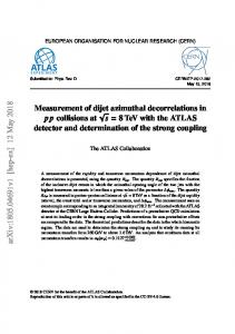
1.1 The Large Hadron Collider accelerator complex The Large Hadron Collider (LHC) is a hadron accelerator and storage ring collider at CERN near Geneva [1]. It is located in the tunnel where previously the Large Electron Positron (LEP) collider had been installed. This tunnel has a circumference of 26659 meters and an internal diameter of 3.7m in the arcs. This constraint essentially did not allow the construction of two completely separate proton rings. Instead, the so called twin-bore magnet design was chosen meaning that the windings for the two beam channels are situated in a common cold mass and cryostat. Because the LHC is a particle–particle collider (and not a particle–antiparticle collider as the Tevatron for example), the magnetic flux has to be directed in the opposite sense for the two beam channels. The schematic layout of the LHC is shown in figure 1.1. The LHC consists of 8 sectors. In the middle of all sectors are the so called long straight sections where the beams can be collided. This will only be done at Interaction Point (IP) 1 for the ATLAS experiment, at IP 2 for the LHCb experiment, at IP 5 for the CMS experiment and at IP 8 for the ALICE experiment. The other long straight sections will be used for beam cleaning, for the beam dump and to house the radio frequency (RF) system. In order to keep the particles on orbit 1232 superconducting dipole magnets are used. These dipole magnets have a nominal field of 8.33 T corresponding to a nominal energy of 7 TeV per beam. The dipole magnets are made up of NbTi Rutherford cables that are cooled down to 1.9 K with superfluid helium. The quality requirements for the dipole magnets are very high. The upper bound on the relative variations of the integrated field, the field shape imperfection and their reproducibility is 10−4 . In addition to the

1

Figure 1.1: The schematic layout of the Large Hadron Collider (LHC).

dipole magnets the LHC magnet system contains a variety of different magnets such as focusing and defocusing quadrupole magnets or chromaticity correcting sextupoles. A full inventory of the LHC magnet system is given in [1]. The primary operation mode for the LHC will be to collide 2 proton beams. From the proton source the protons are first accelerated by the Linac2, then by the Proton Synchrotron Booster (PSB), then by the Proton Synchrotron (PS) and then by the Super Proton Synchrotron (SPS) to an energy of 450 GeV, which is the injection energy into the LHC. Through dedicated transfer lines the protons are injected into the LHC which then accelerates the protons to the design energy of 7 TeV per beam, resulting in √ a center of mass energy of s = 14 TeV for proton–proton collisions. The protons are divided into 2808 bunches where each bunch contains 1.15·1011 protons. This results in a beam current of 0.58 A. The interval between bunch crossings for collisions is 25 ns. In the first year of LHC operation neither the design energy nor the design luminosity will be reached. It is planned to operate at 3.5 TeV per beam at the beginning and then to increase the energy to 5 TeV per beam in the first year of operation. The peak luminosity that will be delivered to the ATLAS and CMS experiments is 1034 cm−2 s−1 , which corresponds to approximately 109 collisions per second. This peak luminosity is unprecedented for a hadron collider and cannot be achieved with a proton– antiproton machine (like the Tevatron) with present day technology. Mainly due to beam loss from collisions the luminosity degrades over time. The estimated luminosity lifetime (the time after the luminosity has fallen to 1/e of the initial luminosity) is estimated to be

2

14.9 h. The expected average turnaround time (time between two runs needed to ramp down the machine and to ramp it up again) is around 7 hours implying an optimum run duration of 12 hours. Together with the assumption of 200 days of machine operation per year and accounting for the uncertainty of the average turnaround time, this yields a maximum total integrated luminosity1 of 80-120 fb−1 per year. Apart from colliding protons the LHC is also able to accelerate and collide fully stripped √ lead (208 Pb82+ ) ions at a center of mass energy of s = 1148 TeV, meaning 2.8 TeV per nucleon per beam. The maximum luminosity for ion–ion collisions that will be delivered at IP8 for the ALICE experiment which is a dedicated heavy ion experiment is 1.0·1027 cm−2 s−1 .

1.2 Experiments at the Large Hadron Collider This section describes the main experiments that will be operated at the LHC. The ATLAS experiment will be presented in chapter 2 in more detail.

1.2.1 ALICE ALICE (A Large Ion Collider Experiment) is a general–purpose detector dedicated to heavy ion physics [2]. It primary will probe quantumchromodynamics (QCD) at extreme energy densities and temperatures which lead to the production of quark–gluon plasma. The schematic layout of ALICE is shown in figure 1.2. ALICE uses the solenoid magnet from the previous L3 experiment at LEP to provide the magnetic field for the central barrel part of the detector. A dipole magnet creates the magnetic field for the forward muon spectrometer. At the interaction point inside ALICE, lead ions will be collided with a center of mass √ energy of s = 1148 TeV at a luminosity of 1027 cm−2 s−1 . This will lead to extreme charged particle multiplicities at mid–rapidity, i.e. close to the plain which containts the inertaction point and is orthogonal to the beam axis. The ALICE detector is designed to operate at charged particle multiplicities up to dN/dη = 8000. The most recent estimate including extrapolations of measurements done by the RHIC detector at the Brookhaven National Laboratory is dN/dη = 1500 − 4000. 1

The integrated luminosity L is defined as the integral of the luminosity over time. The average number of events N for a process for a certain time interval is the product of the integrated luminosity for the time interval and the cross section for the process σ, i.e. N = L σ.

3

Figure 1.2: The schematic layout of the ALICE detector. These high charged particle multiplicities constrained the choice of tracking detectors severely. Three tracking systems are employed in the barrel part of ALICE. The Inner Tracking System (ITS) made up of 6 silicon layers, the Time Projection Chamber (TPC) with a very low material budget and the Transition Radiation Detector (TRD) which also contributes to electron identification. Further systems for particle identification are the Time of Flight (TOF) array using Multigap Resistive Plate Chambers and the High Momentum Particle Identification Detector (HMPID) consisting of proximity–focusing Ring Imaging Cherenkov (RICH) counters. The PHOton Spectrometer (PHOS) is a single–arm high–resolution high–granularity electromagnetic spectrometer consisting of 2 parts. The first is the electromagnetic calorimeter made up of 17.920 PbWO4 crystals. PbWO4 was chosen because of its very small moliere radius and radiation length. The calorimeter is highly segmented and has a depth of 20 radiation lengths. The second is a Charged–Particle Veto (CPV) detector. This is a Multi–Wire Proportional Chamber (MWPC) with a charged particle rejection better than 99%. The primary focus of PHOS is meson identification at low pT and photon identification and energy measurement. The Electro Magnetic CALorimeter (EMCal) is a large Pb–scintillator sampling calorimeter with cylindrical geometry that is read out via wavelength–shifting fibres. Its main goal is to study jets, and in particular the interaction of energetic partons with dense partonic matter. The design criterion for the forward muon spectrometer was a mass resolution of 100 MeV/c2 to allow the separation of all states of heavy quark resonances like

4

0

0

00

J/Ψ, ψ , Υ, Υ , Υ . The forward muon spectrometer covers a pseudo–rapidity range of −4 < η < −2.4. Ten planes of modules are used for the inner muon tracking, four planes of Resistive Plate Chambers for the outer muon tracking.

1.2.2 CMS The Compact Muon Solenoid (CMS) is a general-purpose detector, high luminosity detector [3]. The schematic layout of CMS is shown in figure 1.3.

Figure 1.3: The schematic layout of the CMS detector.

Although the physics program of CMS is very similar to that of ATLAS, very different design decisions have been made. Most striking, CMS will use only one superconducting magnet to produce a 4 T solenoidal field in the central cylindrical region (diameter 6 m, length 12.5 m). The magnet is made of NbTi and the energy stored in it is 2.6 GJ. The Inner Tracking System consists exclusively of silicium detectors. This choice was driven by the granularity, speed and radiation hardness requirements. At design luminosity of 1034 cm−2 s−1 on average 1000 particles will be created from 20 simultaneous proton-proton collisions per bunch crossing. The measurement of the track parameters of all the charged particles and the reconstruction of displaced secondary vertices for τ and b–jet tagging are the main purpose of the Inner Tracking System. Its coverage in pseudo–rapidity is |η| ≤ 2.5. This is achieved by 3 barrel pixel layers and 10 silicon strip larrel layers and their corresponding endcap detectors. In total the Inner Tracking System has an area of active silicon of 200 m2 , making it the largest silicon tracker ever built.

5

The Electromagnetic Calorimeter (ECAL) is a homogeneous scintillation calorimeter. It consists of 61200 PbWO4 crystalls. PbWO4 has a very small radiation length (0.89 cm) and Molire radius (2.2 cm) making it possible to implement a compact design for the ECAL. Furthermore its scintillation decay time is comparable to the LHC bunch crossing time of 25 ns. The scintillation photons are detected by Avalanche Photodiodes (APDs) in the barrel and by Vacuum Phototriodes (VPTs) in the endcaps. A laser monitor system is used to monitor the evolution of the crystal transparency which degrades under irradiation. The information of this system is used for calibration purposes. The Hadronic Calorimeter (HCAL) is a sampling calorimeter using brass as absorber and plastic scintillator as active medium. It is read out via wavelength–shifting fibres. The HCAL and the ECAL are both placed inside the solenoid magnet coil. Due to this restriction an outer hadron calorimeter had to be placed outside of the solenoid magnet to provide a sufficient interaction depth for the barrel region. Two forward detectors are employed. The Centauro And Strange Object Research (CASTOR) detector is a quartz-tungsten sampling calorimeter with a pseudo–rapidity coverage of 5.2 < |η| < 6.6 for diffractive and low–x studies.. The Zero Degree Calorimeter (ZDC) is a quartz-tungsten sampling calorimeter which covers the pseudo–rapidity range |η| ≥ 8.3 for neutral particles contributing to heavy ion and proton-proton diffractive physics. The muon system covers the pseudo–rapidity range |η| < 2.4. In the barrel part |η| < 1.2 Drift Tube (DT) chambers are used. The endcaps are equipped with Cathode Strip Chambers (CSC) because of higher particle rates. Both systems can trigger on the transverse momentum2 pT of muons. In addition, Resistive Plate Chambers (RPC) are also used for triggering purposes. Together with the inner tracking system a good momentum resolution is achieved, about 5% for muons at 1 TeV/c. The charge of the muon can be unambiguously determined up to 1 TeV/c.

1.2.3 LHCb The LHCb experiment will study heavy flavour physics at the LHC [4]. The main point of its physics program is the search for new physics via CP violation and rare decays of beauty and charm hadrons, mainly Bd , Bs and D mesons. The B mesons ¯ production which has a cross section of approx. 500 µb at 14 will be generated via bb 2

6

The transverse momentum pT is defined as the component of the momentum vector that is orthogonal to the beam axis.

TeV center of mass energy for proton-proton collisions. The optimal luminosity for p-p collisions for LHCb is 2·1032 cm−2 s−1 . At this level of luminosity the detector occupancy and radiation damage are kept at a reasonable level and on average there is less then a single proton-proton interaction per bunch crossing. In order to stay at this luminosity level at nominal LHC running conditions the beam focus at the LHCb interaction point can be adjusted independently from the other interaction points. The schematic layout of LHCb is shown in figure 1.4. LHCb is an asymmetric experiment (wrt. η) with an acceptance range of 1.6 < η < 4.9. The magnet that provides the magnetic field for the outer tracking system is a warm magnet. The direction of the magnetic field will be changed periodically in order to control the systematic effects for CP asymmetry measurements.

Figure 1.4: The schematic layout of the LHCb detector.

The tracking system of LHCb consists of 3 parts. The Vertex Locator (VELO) is positioned next to the interaction region and its main purpose is the measurement of tracks in the proximity of the interaction region. These measurements are crucial for the identification of displaced secondary vertices that are characteristic for b and c–hadron decays. The Silicon Tracker consists of two detectors, namely the Tracker Turicensis (TT) and the Inner Tracker (IT). Both of them use silicon microstrip sensors. The TT is positioned upstream of the magnet while the IT is located downstream. Both have small overall material keeping the degradation of the resolution due to multiple scattering at an acceptable level. The Outer Tracker (OT) is designed as a drift time detector using drift tubes filled with a mixture of Argon (70%) and CO2 (30%).

7

Particle identification is provided by two Ring Imaging Cherenkov (RICH) detectors. RICH1 is located upstream of the magnet while the RICH2 is situated downstream. RICH1 uses aerogel and C4 F10 radiators to separate pions from kaons at the low momentum charged particle range from 1 to 60 GeV/c while RICH2 employs CF4 a radiator in the high momentum range from 15 to well above 100 GeV/c. Both use a spherical mirror to reflect the cherenkov photons out of the spectrometer acceptance and than a flat mirror to propagate them to the Hybrid Photon Detectors (HPDs). The HPDs can measure photons at wavelengths of 200–600 nm. The calorimeter system consists of an electromagnetic calorimeter (ECAL) which is a Pb–scintillator sampling calorimeter and a hadronic calorimeter (HCAL) which is an Iron–scintillator sampling calorimeter. Both are read out via wavelength–shifting fibres. The systems contribute to the particle identification of electrons, photons and hadrons and also measure their energy. Prompt photons and π 0 also have to be reconstructed well for flavour tagging. The first muon station is situated right upstream of the electromagnetic calorimeter. A triple Gas Electron Multiplier (GEM) detector is used in its inner region to deal with the expected particle rate. The outer region of the first muon station and the other four muon stations that are downstream of the calorimeters consist of Multi-Wire Proportional Chambers (MWPC). The first three muon stations perform tracking while the two outer most stations are used to identify penetrating particles.

8

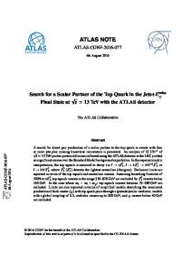
2 The ATLAS Experminent The ATLAS (A Toroidal LHC ApparatuS) detector is a general–purpose detector that will take data from proton–proton collisions at the LHC with a center of mass energy of 14 TeV at a design luminosity of 1034 cm−2 s−1 [5]. The requirements imposed by the physics program of ATLAS are discussed in section 2.1. After describing the magnet system of ATLAS in section 2.2, the three main detector subsystems are presented in the following sections, the Inner Detector in section 2.3, the calorimetry subsystems in section 2.4 and the muon spectrometer in section 2.5. The overall layout of the ATLAS detector is shown in figure 2.1.

Figure 2.1: Cut-away view of the ATLAS detector. The dimensions of the detector are 25 m in height and 44 m in length. The overall weight of the detector is approximately 7000 tonnes. Taken from [5].

9

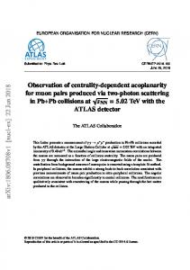
2.1 Physics requirements A primary task of the ATLAS detector is the search for the standard model Higgs boson H which is a benchmark process for many of the subdetectors of ATLAS since the production and decay mechanisms vary considerably as a function of the Higgs boson mass. Important decay channels are H → γγ, H → b¯b and H → ZZ(∗) . The sensitivity of ATLAS for the discovery of a Standard Model Higgs boson in terms of the significance of the signal for Higgs boson decays as a function of the Higgs boson mass and the integrated luminosity is shown in figure 2.2.

−1

Luminosity [fb ]

significance 10

13

ATLAS

9

H → γγ H → ZZ* → 4l H → ττ H → WW → eνµν

8 7

12 11 10 9 8

6

7

5

6 4

5 4

3

3

2

2 1 0

1 120

140

160

180

200

220

240

260

280

300

mH [GeV]

Figure 2.2: Significance contours for different Standard Model Higgs masses and integrated luminosities. The solid curve represents the 5σ discovery contour. The median significance is shown with a colour according to the legend. The hatched area below 2 fb−1 indicates the region where the approximations used in the combination of the four decay channels are not accurate, although they are expected to be conservative.

Searches for physics beyond the standard model will include processes with a transverse 0 0 momentum pT up to a few TeV. For the search for new heavy gauge bosons W and Z

10

through their lepontic decays this means that the resolution and charge identification must still be accurate in this high momentum range. The search for quark compositeness involves very high pT jets and requires a good linearity for jet energies up to several TeV. Another variable sensitive to physics beyond the standard model is the missing transverse energy1 ETmiss . For supersymmetric models2 where the R-parity is conserved, the decay of supersymmetric particles would proceed in cascades where the lightest stable supersymmetric particle (LSP) would not be able to decay any further and would escape the detector nearly without interacting with the detector therefore creating a significant ETmiss . Other models that have experimental signatures including a significant ETmiss are extra dimensions models and quantum gravity. The ATLAS detector will also perform high precision tests of the standard model of particle physics. Among the properties to be measured are the top quark mass, the top quark spin and the W boson mass with a desired precision of 10 MeV. At the design luminosity of 1034 cm−2 s−1 approximately 23 inelastic proton–proton collisions will occur at each bunch crossing. Together with a bunch crossing spacing of 25 ns this will result in a enormous particle production rate that requires a highly efficient trigger system to detect events of interest over the large background as well as fast and radiation hard sensors and electronics. All the benchmark processes mentioned above lead to the following requirements for the ATLAS detector, see table 2.1: 1. Large acceptance in ϕ and in pseudorapidity for a good ETmiss resolution. 2. Good charged-particle momentum resolution, charge identification and reconstruction efficency in the inner tracker. Good resolution for secondary vertices for τ 1

Since the detector inertial system is the center of mass system of the colliding protons, the vector sum of the momenta of all particles is zero for each proton-proton collision. Since the detector does not cover a small stereo angle around the beam axis, the sum of the momenta of the particles in the detector acceptance region can be deviate from 0. However, the transverse component of the momenta in the uncovered regions is very small. As a consequence the sum of the transverse momenta of the particles in the detector acceptance region is always very close to 0. If a particle has significant momentum and escapes the detector unmeasured, i.e. a neutrino, the sum of the measured transverse momenta is not zero and this is denoted missing transverse energy, ETmiss . 2 Supersymmetry is the concept for an invariance that links fermions and bosons. Every fermion has a bosonic supersymmetric partner and every boson has a fermionic supersymmetric partner. The main advantage of Supersymmetry is that the loop corrections in the Higgs mass renormalization cancel exactly due to the opposite sign for fermions and bosons, therefore solving the hierarchy problem in an elegant way.

11

and b-jet tagging. 3. Excellent electromagnetic calorimetry for electron and photon identification and measurements. 4. Hadronic calorimetry with large coverage for jet and ETmiss measurement. 5. Good muon momentum resolution, charge identification and reconstruction efficency in the muon spectrometer up to the TeV range. 6. The electronics and sensor elements must be fast and radiation–hard due to the experimental conditions at the LHC. 7. Efficient trigger also for low pT objects with sufficient background rejection. Turning these requirements into numbers yields the required performance listed in table 2.1. Detector component Tracking Electromagnetic calorimetry Hadronic calorimetry barrel and endcap forward Muon spectrometer

Resolution σpT /pT = 0.05%p √ T ⊕ 1% σE /E = 10%/ E ⊕ 0.7%

η measurement |η| < 2.5 |η| < 3.2

η trigger

√ σE /E = 50%/√E ⊕ 3% σE /E = 100%/ E ⊕ 10% σpT /pT = 10% at pT =1 TeV

|η| < 3.2 3.1 < |η| < 4.9 |η| < 2.7

|η| < 3.2 3.1 < |η| < 4.9 |η| < 2.4

|η| < 2.5

Table 2.1: Required performance of the ATLAS detector. The unit for E is GeV, the unit for pT is GeV/c.

2.2 Magnet System In contrast to the CMS detector, where only one solenoidal field is used, the ATLAS detector employs a unique hybrid system of four superconducting magnets to provide the magnetic field for the inner tracking detector called Inner Detector and the muon spectrometer. The total size of the magnetic system in 22 m in diameter and 26 m in length. The stored energy in the system im 1.6 GJ. Central solenoid The central solenoid provides the solenoidal field for the momentum measurement in the Inner Detector. The solenoidal field is aligned with the beam axis and has a nominal

12

strength of 2 T. The superconducting cables are made out of Al–stabilized NbTi. The central solenoid is located inside the electromagnetic barrel calorimeter. In order to achieve the required performance of the electromagnetic barrel calorimeter, the material budget of the central solenoid is crucial. A thickness of only 0.66 radiation lengths at normal incidence has been achieved.

Barrel toroid The barrel toroid provides the toroidal field for the momentum measurement in the barrel part (|η| < 1.4) of the muon spectrometer. The bending power provided by the barrel toroid is 1.5 to 5.5 Tm. The eight coils of the barrel toroid are housed in eight separate cryostats. These are linked together by a support structure to deal with the Lorentz force which amounts to the equivalent of 1400 tonnes.

Endcap toroids The two endcap toroids provide the toroidal field for the momentum measurement in the endcap part (1.6 < |η| < 2.7) of the muon spectrometer. The bending power provided by the endcap toroids is 1 to 7.5 Tm. In the transition region (1.4 < |η| < 1.6) the magnetic fields of the barrel and the endcap toroids overlap and the provided bending power is lower than in the other regions.

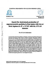
2.3 Inner Detector At the design luminosity of the LHC approximately 1000 particles will emerge from the collision point every 25 ns. The primary task of the Inner Detector is to measure the tracks of the charged particles. Based on these tracks, the Inner Detector will measure the transverse momentum of charged particles down to a transverse momentum pT of 0.5 GeV/c. It will reconstruct the primary vertex as well as secondary vertices, e.g. from τ leptons, b–quarks or c–quarks, if present. Furthermore the Inner Detector will contribute to electron identification by measuring transistion radiation. The bending power required for the momentum measurement is provided by the central solenoid. The layout of the Inner Detector is shown in figure 2.3.

13

Figure 2.3: Cut-away view of the ATLAS Inner Detector. Taken from [5]. Pixel Detector The Pixel detector is a sillicon detector consisting of 1744 pixels sensors with 46080 readout channels per sensor. The barrel part features three cylindrical layers, the two endcaps three discs each. The thickness is 250 µ with a nominal pixel size 50x400 µm2 . The Pixel detector will provide discrete space–points that will be used for high resolution tracking. The standard bias voltage is 150 V, although after 10 years of operation up to 600 V will be needed for good charge collection to compensate the degradation of the performance due to radiation damage.

Silicon Microstrip Tracker The Silicon Microstrip Tracker (SCT) is also a sillicon detector consisting of 15192 sensors with 768 strips per sensor. The barrel part features four cylindrical layers, the two endcaps 9 discs each. The thickness is 285 µm. The SCT will provide stereo pairs to the tracking algorithms. The standard bias voltage is 150 V, although after 10 years of operation up to 350 V will

14

be needed for good charge collection to compensate the degradation of the performance due to radiation damage. Transition Radiation Tracker The Transition Radiation Tracker (TRT) consists of polyimide drift tubes of 4 mm diameter. They are operated at 1530 V resulting in a gain factor of 2.5x104 and provide R − ϕ information only. The chosen gas mixture is 70% Xe, 27% CO2 and 3% O2 at 5-10 mbar over–pressure. The TRT covers the pseudorapidity range of |η| < 2.0 and has 351000 readout channels. In addition to providing typically 36 hits per track to the tracking algorithms, the TRT also contributes to the electron identification. The low energy transition radiation photons emitted by traversing electrons are absorbed in the gas mixture and yield much larger signal amplitudes for electrons than for minimum ionizing charged particles. The electron identification capabilities are implemented by using a high threshold to detect the enhanced signal for electrons in addition to a low threshold for identifying standard hits for tracking.

2.4 Calorimetry All calorimeters employed by ATLAS are sampling calorimeters. The electromagnetic (subsection 2.4.1) and hadronic (subsection 2.4.2) calorimeters cover the pseudorapidity range of |η| < 4.9. The layout of the calorimetry system is shown in figure 2.4.

2.4.1 Liquid Argon Electromagnetic Calorimeter The Liquid Argon Electromagnetic Calorimeter is a sampling calorimeter using lead as the absorber and liquid argon as the active material. It consists of a barrel part (|η| < 1.475) and two endcaps (1.375 < |η| < 3.2). A special geometry (accordion) has been developed to provide complete ϕ symmetry without azimuthal cracks has been chosen for the barrel and the endcaps. The Liquid Argon Electromagnetic Barrel Calorimeter (LAr EMB) is described in chapter 4 in more detail since the calibration of the electron energy measurement with the LAr EMB in the Combined Test Beam 2004 is the subject of chapter 5. Each endcap consists of two co–axial wheel–like structures. The outer wheel (1.375
0.8. The width of the liquid argon gap is 2.12 mm for each side of the read-out electrode. The read-out electrodes consist of three copper layers that are glued together and are separated by Kapton layers. The inner layer acts as the signal layer and is isolated from the other two high voltage layers. The nominal setting for the potential between the electrode high voltage layers and the absorbers (ground) is 2000 V. HV

Signal

Lead Prepreg Steel

Liq uid

Steel Prepreg

Arg on G

ap

Ground

Copper Kapton

Figure 4.2: Schematic layout of the absorber, the liquid argon gap and the read-out electrode (three layers glued together).

The signal is induced in the read-out electrodes by the drift of the ionization electrons in the electric field created by the high voltage.

4.2.2 Presampler Since there is a significant amount of material in front of the electromagnetic calorimeter, the amount of energy deposited in this material has to be estimated. This is done using a presampler that is placed in front of the accordion calorimeter. The presampler is a thin (11 mm) active layer of liquid argon enclosed by a 0.4 mm thin glass-epoxy shell.

31

The procedure how the presampler is used to estimate the energy deposited upstream electromagnetic calorimeter is described in section 5.7.1

4.2.3 Granularity The ATLAS Electromagnetic Barrel Calorimeter is longitudinally segmented into three layers, called the strip, middle and back layer or also sampling 1, sampling 2 and sampling 3. A sketch is shown in figure 4.3. The granularity in the η − ϕ plane is different for the three layers and reflects the trade– offs between the required position resolution and shower shape identification on the one side and the number of readout channel on the other. The granularity of the strip layer is very fine in η, providing a good angular resolution in the η direction and π 0 rejection capabilities. The middle cells are also used for seeding clusters for the trigger since most of the energy is deposited in this layer for electrons and photons above approximately 10 GeV (depending on η). The thickness of the ATLAS Electromagnetic Barrel Calorimeter varies from 22 radiation lengths (barrel) to 33 radiation lengths (gap region). Layer Strip Middle Back

∆η 0.025/8 0.025 0.05

∆ϕ 2π/64 2π/256 2π/256

Depth (radiation lengths) 2.5-4.5 16.5-19 1.4-7

Table 4.1: Granularity for the three layers of the ATLAS Electromagnetic Barrel Calorimeter.

4.3 Signal shape The signal is induced by the drift of the ionization electrons in the electric field in the liquid argon gaps. Its approximately triangular shape is shown in figure 4.4(a). Right after the signal is amplified by the preamplifier it is transformed by a shaping amplifier in order to optimize the signal-to-noise ratio. The triangular signal is transformed into a narrow peak and a long undershoot (see figure 4.4(b)). The signal is sampled only in the vicinity of the peak because the amplitude of the peak is proportional to the energy deposit in the cell [13]. The calibration of the read out chain is discussed in section 5.5.

32

Cells in Layer 3 ∆ϕ×∆η = 0.0245×0.05 Trigge r Towe ∆η = 0 r .1

2X0

47 0m

m

η=0

16X0 Trigge Tow r ∆ϕ = 0er .0982

m

m

4.3X0

15

00

1.7X0 ∆ϕ=0.0 245x 36.8m 4 mx =147.3 4 mm

ϕ

Square cells in Layer 2 ∆ϕ = 0

.0245

∆η = 0 .025 m/8 = 4.69 m m ∆η = 0 .0031 Strip cells in Layer 1

37.5m

η

Figure 4.3: Sketch of a barrel module of the electromagnetic calorimeter. The accordion structure and the granularity in η and ϕ of the cells of each of the three layers is shown.

33

Figure 4.4: Signal (a) induced by the drift of the ionization electrons in the electric field in the liauid argon gaps and the signal after shaping (b). The black circles indicate the sampling points of the shaped signal.

34

5 Calibrating the Electron Energy Measurement for the Combined Test Beam 2004 This chapter describes the calibration of the electron energy measurement for the Combined Test Beam (CTB) 2004 in the presence of a magnetic field in the Inner Detector. The whole calibration chain for the electron energy measurement in ATLAS consists of the following three consecutive steps: 1. Calibration of the readout channels, also called electronic calibration. 2. Calibration of the energy response of the whole electromagnetic calorimeter. 3. Further calibration using physics events in ATLAS from LHC collision data, e.g. electrons from Z→ee decays to calibrate the absolute scale or inclusive electrons using E/p to calibrate the relative scale between the Inner Detector and the electromagnetic calorimeter. This chapter focuses on calibration of the energy response of the whole electromagnetic calorimeter (item 2) and therefore the term calibration will be used in this chapter for this aspect of the calibration chain. For an electron impinging the detector a cluster of cells, i.e. readout channels, is formed and associated to the electron. Based on the energies from the cells in the cluster the inital energy, denoted calibrated cluster energy, of the electron is computed. The sequence of procedures for this computation is shown in figure 5.1. After a brief description of the setup (section 5.1) and the data samples (section 5.2), the event selection (section 5.3) and beam related weighting procedures (section 5.4) are presented. Section 5.5 recapitulates the way the energy deposited in a single calorimeter cell is measured and how clusters are formed out of these cells. This is followed by a comparison of the Monte Carlo simulation to data (section 5.6). Finally a Monte Carlo

35

MC simulation

Data

Readout channel calibration

Calibration runs

Cell Energies

Cell Energies

Clustering

Visible Cluster Energies

Readout channel calibration

Clustering

Calibration Hits Method

Visible Cluster Energies

Cluster Calibration

Cluster Calibration

Calibrated Cluster Energy

Calibrated Cluster Energy

Figure 5.1: Sequence of procedures to compute the calibrated cluster energy. The Readout channel calibration and the Clustering are briefly discussed in section 5.5. The Calibration Hits Method and Cluster calibration are presented in section 5.7. Monte Carlo simulation to data comparisons are discussed in section 5.6 for the Visible Cluster Energies and in section 5.8 for the Calibrated Cluster Energy. based calibration procedure for the cluster energy is presented in section 5.7 and applied to data in section 5.8 in order to extract the linearity and resolution for the liquid argon calorimeter in the presence of a magnetic field in the Inner Detector.

5.1 The Combined Test Beam 2004 During the Combined Test Beam 2004 data was taken from June until November 2004. The data that is used in this thesis comes from the last data taking period where all sub detectors participated. A sketch of the fully combined setup is shown in figure 5.2, including the coordinate system for the CTB 2004. A detailed description of the CTB

36

2004 can be found in [14]. The fully combined setup consisted of the following compoAdditional material for LAr material study and position of BIS chamber

y

x

z

00 11 11 00 00 11 00 11 00 11 00 11 00 11

Inclination of cryostat = 11.25o

Figure 5.2: Setup of the Combined Test Beam 2004. nents [15]: Pixel detector Two modules for each of the three pixel layers (B, 1 and 2 as defined in [16]), adding up to six pixel modules in total. Semiconductor Tracker (SCT) Two modules for each of the four layers of the SCT [17], meaning 8 modules in total. Transition Radiation Tracker (TRT) Two barrel wedges, constituting 1/8 of a barrel wheel [18]. LAr electromagnetic barrel calorimeter (LAr EMB) One module, constituting 1/16 of a barrel wheel [19]. Tile calorimeter Three long barrel modules and three extended barrel modules, constituting 3/98 of a barrel wheel [20]. Muon spectrometer Three stations of monitored drift tube barrel chambers and three stations of monitored drift tube endcap chambers. For some runs, including the runs used in this analysis, a monitored drift tube BIS type chamber was positioned in front of the LAr EMB cryostat.

37

The CTB 2004 setup included a magnet in order to evaluate the performance of the various detector sub systems in the presence of a solenoidal magnetic field in the Inner Detector like it will be the case for the full ATLAS detector taking data from LHC collisions. The MBPS magnet produced a field for the pixel and SCT modules. The magnetic field was directed in such a way that charged particles passing through the pixel and SCT detector were deviated in ϕ (angle in the y–z plane). Contrary to the full ATLAS setup, the TRT was not positioned inside the magnetic field. In order to be able to measure the response of the calorimeters to particles impinging at different η 1 positions the electromagnetic and hadronic calorimeter modules were mounted on a movable table that could be rotated in θ (angle in the x–z plane) and translated along the x–direction. The electrons for the runs that are used in this analysis have been provided by the CERN H8 beam line. The H8 beam is created by directing 400 GeV/c protons from the CERN Super Proton Synchrotron (SPS) onto a primary target made of up to 300 mm of Beryllium. The emerging secondary beam has momenta between 9 GeV/c and 350 GeV/c. The beam line that uses this beam is called the high energy beam line. A sketch of the H8 beam line instrumentation is shown in figure 5.3, a detailed description ˇ is given in [21]. The high energy beam line was equipped with two Cerenkov counters. CHRV1 was furthest upstream and is not shown in figure 5.3. CHRV2,HE was located 1 m upstream of the last bending magnet of the VLE spectrometer. The beam profile was determined using four beam chambers (BC-1, BC0, BC1 and BC2). The main trigger consisted of three scintillators (S1, S2 and S3). In order to reject muon halo from the beam a scintillator (SMH) with a hole of 3.4 cm in diameter was used in anti-coincidence with S1,S2 and S3. The momentum selection for the high energy beam line is performed using a spectrometer consisting of two collimators and two triplets of bending magnets [14]. The momentum selection for the high energy beam line is done 400 m upstream of the Combined Test Beam 2004 setup. Between the collimator that performs this selection and the setup, the beam particles traverse air, four mylar windows of two beam pipes ˇ and one Cerenkov counter CHRV1. These contributions add up to 15% of a radiation length and are collectively denoted as far upstream material. Since the beam line optic for these 400 m has been designed for the nominal beam momentum and the fact that 1

The pseudo rapidity η is defined by η = −ln tan θ2 where θ is the angle in the x–z plane.

38

Figure 5.3: H8 beam line instrumentation. The straight line represents the high energy beam line that was used for the data analyzed in this thesis. Run number pnominal η nominal MBPS current beam (GeV/c) (A) 2102399 100 0.45 -850 2102400 50 0.45 -850 2102413 20 0.45 -850 2102452 80 0.45 -850

Events 200000 200000 70000 200000

< pbeam > σ(pbeam ) (GeV/c) (GeV/c) 99.80 ± 0.11 0.24 50.29 ± 0.10 0.12 20.16 ± 0.09 0.05 80.0 ± 0.10 0.19

Table 5.1: Run number, nominal beam momentum, nominal η impact position, current in the MBPS magnet that provides the field for the inner detector, total number of events taken, estimated average beam momentum and beam spread for the data samples used in this analysis. some particles loose energy (and therefore momentum) while traversing the far upstream material, the acceptance of this part of the beam line has to be taken into account in the simulation. This is described in subsection 5.4.1.

5.2 Data samples The data samples that were taken during the CTB 2004 and used for the analysis in this thesis are listed in table 5.1. The average beam momentum < pbeam > and the beam spread σ(pbeam ) was computed for each run using the collimator currents from the beam momentum selection spectrometer described in section 5.1.

5.3 Event selection This section describes the event selection procedure for the CTB 2004. Subsection 5.3.1 is devoted to particle identification for electrons, subsection 5.3.2 describes the require-

39

ments concerning the beam quality and subsection 5.3.3 deals with detector imperfections. Finally subsection 5.3.4 discusses the quality requirements for reconstructed electron–like objects.

5.3.1 Particle identification The purpose of the procedures described in this subsection is to select only events for the analysis that are triggered from an electron from the beam entering the calorimeter. Requirements concerning measurement variables from the beam line instrumentation present only in the data samples are only applied there. Requirements that involve measurement variables from the calorimeters or the inner detector are applied both to the data and to the simulation samples in order to avoid introducing any bias. Where this has not been possible it is explicitly stated. The following requirements have to be met for an event to be accepted: 1. Less than 700 MeV are deposited in the first tile calorimeter layer. The purpose of this requirement is to reject pions. 2. Less than one percent of the energy deposited in the calorimeters is deposited in the tile calorimeter. The purpose of this requirement is to reject pions. 3. There must be at least 20 hits in the TRT. The purpose of this requirement is to be sure to have a good track in the TRT. 4. TRT High Level Hit Probability> 0.15: The purpose of this requirement is to reject pions and muons. This requirement is applied only to the data samples, since the TRT High Level Hit Probability is not correctly modeled in the simulation, and only electrons have been simulated. 5. Trigger from the trigger scintillators S1∧S2: This requirement guarantees that only beam particle triggered events are considered and not random tirggers that were injected to measure pedestal levels. Since the trigger scintillators are not simulated, the requirement is applied only to the data samples. 6. Muon halo veto scintillator (SMH) < 460 ADC: The purpose of this requirement is to reject muons. Since the muon halo veto scintillator is not simulated, the requirement is applied only to the data samples. 7. Cherenkov counter CHRV2,HE > 650 ADC: The purpose of this requirement is to reject pions for the run at 20 GeV/c nominal beam momentum. Since the

40

cherenkov counter is not simulated, the requirement is applied only to the data samples.

5.3.2 Beam quality

50

dN (mm−1) d∆ xBC−1

xBC−1 (mm)

Two additional cuts2 are applied to the data to ensure that only particles from the central part of the beam and no particles from the beam halo are used. 40 30 20

105

Constant 8.484e+04 ± 296 Mean −2.983± 0.002 Sigma 0.6624 ± 0.0014

104 103

10 0

102

−10 −20

10

−30 −40 −50 −20 −15 −10 −5

0

5

1 −60

10 15 20

−20

0

20

40

60

(mm−1)

Constant1.717e+04 ± 83 Mean 45.53 ± 0.01 Sigma 2.154 ± 0.008

BC−1

(mm)

104

dN d∆ y

−20

y

BC−1

−10

−40

∆ xBC−1 (mm)

x BC0 (mm)

−30

103

−40 102

−50 −60

10

−70 −80 −20 −15 −10 −5

1 0

5

10 15 20 y (mm) BC0

0

10 20 30 40 50 60 70 80 ∆y (mm) BC−1

Figure 5.4: Beam chambers BC-1 vs. BC0 x (top left) and y (bottom left) measurements with fitted line. Distribution of the orthogonal distances (∆xBC-1 and ∆yBC-1 ) from this line for x (top right) and y (bottom right) values together with a Gaussian fitted to the core of the distribution. 1. The x values measured by the beam chambers BC-1 and BC0 are linearly correlated since the setup is rigid and there is no magnetic field in the flight path between these two beam chambers. The same is true for y values. The left plots of figure 5.4 show the distributions for x and y. A line is fitted to each of the distributions and the orthogonal distances (∆xBC-1 and ∆yBC-1 ) are plotted in the right plots of figure 5.4. Gaussians are fitted to the orthogonal distance distributions and 3 times the σ of a Gaussian is defined as the largest allowed absolute orthogonal 2

The term cut refers to a requirement to has to be fulfilled for an event to be considered for the analysis. If the requirement is not fulfilled, the event is cutted away from the analysis.

41

dN (mm−1) d∆ xBC−1

xBC−1 (mm)

20 15 10

Constant 2929 ± 12.3 Mean −3.03 ± 0.00 Sigma 0.4961 ± 0.0014

103

5 102

0 −5 −10

10

−15 −20 −20 −15 −10 −5

0

5

10 15 20

−4.5 −4 −3.5 −3 −2.5 −2 −1.5 ∆ xBC−1 (mm) (mm−1)

Constant 2624 ± 12.3 Mean 45.49 ± 0.01 Sigma 1.92 ± 0.01

BC−1

−30 −35

dN d∆ y

y

BC−1

(mm)

x BC0 (mm)

−40

103

−45 102

−50 −55 −60

10

−20 −15 −10 −5

0

5

10 15 20 y (mm) BC0

40

42

44

46

48

50 ∆y

BC−1

52 (mm)

Figure 5.5: Beam chambers BC-1 vs. BC0 x (top left) and y (bottom left) measurements with fitted line with 3σ cut applied. Distribution of the orthogonal distances (∆xBC-1 and ∆yBC-1 ) from this line for x (top right) and y (bottom right) values together with a Gaussian fitted to the core of the distribution. pnominal (GeV/c) beam 20 50 80 100

(min,max) BC1x (mm) (min,max) BC1y (mm) (−15, +7) (−13, +12) (−15, +5) (−15, +15) (−5, +7) (−10, +10) (−15, +7) (−15, +15)

Table 5.2: Allowed ranges for the x and y values (denoted BC1x and BC1y ) of beam chamber BC1 for all beam momenta.

distance. The x and y distributions and the corresponding orthogonal distance distributions with these cuts applied are shown in figure 5.5.

2. The x and y values (denoted BC1x and BC1y ) of beam chamber BC1 are restricted to ranges where the total visible energy in the electromagnetic calorimeter is flat with respect to BC1x and BC1y . The intervals used are given in table 5.2.

42

5.3.3 Detector imperfections This subsection describes the procedures to discard events that have been affected by detector imperfections. Coherent noise in the presampler This cut is used to reject events with coherent noise in the presampler layer. In order to achieve this, the distribution of the presampler cell energies of all cells outside the region where the beam hits the calorimeter is considered, i.e. |ηcell − ηbeam | > 0.2. If there is no coherent noise present, this distribution is a Gaussian with mean equal to 0 and an rms equal to the average noise of the cells. Let n+ P S denote the number of presampler − cells with positive energy +and −nP S the number of presampler cells with negative energy. n −n An event is rejected if n+P S +n−P S > 0.6. Since the coherent noise is not simulated this PS PS cut is only applied to the data samples. Shaper problem The cells at 0 < ϕcell < 0.1, ηcell = 0.3875 in the middle layer suffered from an unstable signal shaper. The stochastic distortion of the signal shape introduced a variation of the order of 3% for the gain values. Although the effect on the reconstructed cluster energy is fairly small, all events with clusters that contain any of these cells are discarded. In order not to introduce a bias this cut is applied both to the data samples and to the simulation samples.

5.3.4 Quality of reconstructed objects The purpose of the requirements described in this subsection is to select events that have a reconstructed electron–like object. This object consists of a cluster in the electromagnetic calorimeter and a track in the Inner Detector that is geometrically matched to the cluster. Track to cluster matching A track in the inner detector can be extrapolated to the liquid argon calorimeter and the η and ϕ coordinates of this extrapolation can be computed. In order for a track to be matched to a cluster the following two conditions are imposed • |ϕT rack − ϕCluster | < 0.05 rad,

43

• |ηT rack − ηCluster | < 0.01. For each event all possible track–cluster combinations are tested whether the track matches to the cluster or not. The event is accepted for the analysis if there is at least one matched track-cluster combination. Track quality At least 2 hits in the pixel detector for the matched track are required. This requirement ensures an acceptable track quality.

5.4 Event weighting This section discusses two weighting schemes that are applied for the CTB 2004. In general, a weighting scheme is a technique in statistical data analysis where a number, i.e. a weight, is assigned to each data item of the analysis. The weight reflects the relative importance of the corresponding data item. As a consequence, some data items are more emphasized than others. In the case of this analysis, a weight is assigned to each event. Since a combination of weighting schemes is employed, the total weight of an event is the product of the individual weights computed by all weighting schemes for the given event. For some distributions, e.g. the impact profiles, there is a difference between the simulated Monte Carlo samples and the data samples. The purpose of the event weighing is to make these samples comparable. In order to achieve this, the events in the two samples are weighted in such a way that the differences between the simulated Monte Carlo samples and the data samples vanish for the distributions mentioned above. A weighting scheme to describe the beam line acceptance is presented in subsection 5.4.1. The angular weighting procedure introduced in subsection 5.4.2 is used to match the impact profiles of the Monte Carlo simulation to data.

5.4.1 Beam line acceptance Particles which loose a signficant amount of energy in the beam line will have a smaller probability to reach the trigger scintillators. Since the beam line was not modeled in the Monte Carlo simulation, a weighting scheme is employed to simulate the acceptance of the beam line. In the simulation a detector is placed directly after the far upstream material (see section 5.1 and subsection 5.6.1). For each event the ratio of the energy of the

44

most energetic particle E˜ measured by this detector and the nominal beam energy, i.e. ˜ nominal , is used to compute a weight from the weighting curve shown in figure 5.6. E/E beam

Weight (%)

This weight is attributed all measurement variables of the event. The weighting curve has been obtained by a dedicated beam line simulation beforehand [22]. The application of the beam line acceptance weight has no significant impact on the calorimeter measurements, but is needed for a correct description of the tail of the momentum measurement in the inner detector (see figure 5.7).

100 90 80 70 60 50 40 30 20 10 0 20

30

40

50

60

70

80

90

100

~ E / Enominal (%) beam

Figure 5.6: Beam line acceptance weight function.

5.4.2 Angular weighting The beam profile is modeled in the Monte Carlo simulation to reflect the real beam profile. Since this is possible only to a certain extent an additional weighting scheme is introduced. For the data and the Monte Carlo sample for a given nominal beam momentum, the η and ϕ distributions of the clusters (see subsection 5.6.2) in the calorimeter are computed and binned into histograms. In order to obtain the best angular resolution possible, the strips layer cells are used for the computation of η and the middle layer cells for the computation of ϕ. For each bin in the η and ϕ histograms a weighting

45

normalized number of events

0.12 Data 0.1 Simulation Simulation without Acceptance

0.08

0.06

0.04

0.02

0 0.04

0.05

0.06

0.07

0.08

0.09 -1 1 p (c GeV )

Figure 5.7: The ration of 1/p measured with the silicon detector (3 pixel layers and 4 SCT layers) for a beam momentum of pbeam =20 GeV/c. The solid circles are the data, the shaded area represents the simulation including the beam acceptance, the dashed line the simulation without the beam acceptance. The remaining discrepancy between the Monte Carlo simulation including the beam acceptance and the data comes from a slight misalignment of the Inner Detector.

factor is computed in the following way: If the bin content for the Monte Carlo sample is larger than for the data sample, this bin gets the ratio between data content and Monte Carlo simulation content (which is by definition smaller than 1) as weight for the Monte Carlo sample and 1 as weight for the data sample. If the bin content for the data sample is larger than for the Monte Carlo sample, it is done the other way round. This ensures that the distributions for the Monte Carlo and the data samples are equal after weighting and that all weights that are used are ≤ 1, therefore avoiding numerical instabilities. For each event that is accepted for the analysis all measurement variables are weighted with these weighting distributions where the η and ϕ position of the cluster is used to determine the bins whose weights are used.

46

5.5 Energy measurement The calibration of the energy measurement of the LAr calorimeter consists of two consecutive steps. First the raw signal (in ADC counts) for each cell is converted into the deposited energy in the cell. This step is denoted as electronic calibration and shortly discussed in subsection 5.5.1. During the second step clusters are formed out of calorimeter cells and an estimate of the initial energy of the impinging particle associated with the cluster is computed. The cluster formation algorithm is briefly described in subsection 5.5.2 and section 5.7 is devoted to a Monte Carlo simulation based procedure for computing the estimate for the initial energy of the particle.

5.5.1 Electronic calibration A very detailed discussion of the electronic calibration and cell energy reconstruction for the LAr EMB calorimeter is given in [23]. The signals that are induced by the drifting ions in the liquid argon gaps of the calorimeter are amplified, shaped and then digitized at a sampling rate of 40 MHz in one of the three available gain channels. In the CTB 2004 setup six samples are digitized in contrast to ATLAS where five samples are digitized. From these six samples in the CTB 2004 five samples si closest to the signal peak are chosen and the signal amplitude ADCpeak is computed by the Optimal Filtering Method [24] ADCpeak =

5 X

ai (si − p)

(5.1)

i=1

where ai are the optimal filtering coefficients that are computed from the predicted ionization pulses obtained using the technique described in [25] and p is the pedestal value which is the mean of the signal values generated by the electronic noise that is measured in dedicated calibration runs. From the signal amplitude ADCpeak the cell energy Ecell is computed by 1 X Ecell = FDAC→µA FµA→MeV MP hys Ri [ADCpeak ]i

(5.2)

MCal i=1,2

where the factors Ri model the electronic gain with a second order polynomial, converting P hys the ADCpeak amplitude into the equivalent current units (DAC). The factor MMCal takes the difference between the amplitudes of a calibration and an ionization signal of the

47

same current for the electronic gain into account [25–28]. The constants FDAC→µA and FµA→MeV finally transform the current (DAC) into energy (MeV). The details of the computation and validation of all the calibration constants used in equations 5.1 and 5.2 are described in [23]. The conversion factor FµA→MeV between the current measured by the LAr readout cells and the corresponding deposited energy3 applied in the data reconstruction is taken from the 2002 liquid argon standalone test beam [29]. This conversion factor depends on the temperature of the liquid argon in the cells and during the 2002 liquid argon standalone test beam this temperature was not known with a precision of 0.1 K like at the Combined Test Beam 2004. The absolute energy scale of the LAr calorimeter was therefore extracted from CTB 2004 data. The scale factor is computed by comparing Monte Carlo simulation to data for runs with a nominal beam momentum of 180 GeV/c taken in different periods of the Combined Test Beam 2004. The computation yields a scale factor of 1.038±0.007. The error of 0.7% is composed of • the uncertainty of the spectrometer current measurement for these runs, 0.04%, • the uncertainty of the absolute scale of the beam momentum selection for pbeam = 180 GeV/c, 0.52%, • the response uniformity of the calorimeter, 0.4%.

5.5.2 Cluster building In order to reduce the noise contribution to the energy measurement, a finite number of cells is used to calculate the energy. The process of choosing which cells are used is called cluster building. Several methods exist, e.g. topological clustering and sliding window clustering. Here a sliding window algorithm is used. For building clusters of calorimeter cells that correspond to the impinging electron the standard ATLAS clustering [30] is used. For electrons, this means that a window of 3x7 middle cells (ηxϕ extension) is slided across the calorimeter and the position with the highest energy content is used as seed position for the cluster. This seed is propagated to the other layers of the calorimeter. For each layer, cells contained in windows centered at the given seed for the layer are added to the cluster. The size of the window is different for the various layers. 3

This factor contains an average sampling fraction, hence Ecell is a rough estimate of the energy deposited in this cell. In reality, the sampling fraction depends on the initial energy of the incident particle and will be corrected afterwards (see section 5.7).

48

5.6 Monte Carlo simulation and comparison to data This section is devoted to the Monte Carlo simulation of the CTB 2004. After a description of the Monte Carlo simulation setup in subsection 5.6.1, the results of the Monte Carlo simulation are compared to data taken in the CTB 2004. This comparison is performed for the impact profile (subsection 5.6.2), the energy response for the different layers of the calorimeter (subsection 5.6.3) and the development of the electromagnetic shower (subsection 5.6.4). The Monte Carlo simulation to data comparison for the momentum measured by the Inner Detector is presented in subsection 5.6.5 because this measurement is one of the ingredients for the intercalibration procedure presented in chapter 6. Since the calibration procedure (section 5.7) relies on Monte Carlo simulation a sufficiently good agreement between the Monte Carlo simulation and the data is necessary to achieve the required level of accuracy for the electron energy measurement. For the required linearity of 5h the agreement between the Monte Carlo simulation and the data for the sum of the visible energies of all cells in a cluster also has to be at the level of 5h.

5.6.1 Monte Carlo simulation of the Combined Test Beam 2004 The response of the detector setup of the Combined Test Beam 2004 to the various beam particles is simulated using the GEANT4 toolkit [31]. GEANT4 uses Monte Carlo methods to simulate the physics processes when particles pass through matter. The QGSP-EMV physics list was used to parameterize these physics processes. The details of the geometric description of the Combined Test Beam 2004 in GEANT4 are described in [32]. The simulated energy deposits are reconstructed with the same software as the data. This is all done inside the ATLAS offline software framework ATHENA, release 12.0.95. The far upstream material (section 5.1) is taken into account with a piece of aluminum with the equivalent thickness of 15% of a radiation length placed directly downstream of the GEANT4 particle generator. All particles that emerge from the far upstream material are recorded in the simulation and are used to model the effect of the beam line acceptance (subsection 5.4.1). One effect that is not modeled in the simulation is the cross talk between strip and middle layers. This cross talk has been measured by analyzing the response of the various cells

49

to calibration pulses [33, 34]. A Middle-to-Strips cross-talk of Xmi→st = 0.05 % and a Xst→mi = 0.15 % Strips-to-Middle cross-talk have been obtained (peak-to-peak values). They are accounted for after the energy reconstruction by redistributing 8·Xmi→st ·EMiddle from the middle layer energy4 to the strip layer energy5 and Xst→mi · EStrips from the strip layer energy to the middle layer energy. The simulated electron momentum that is used in the Monte Carlo simulation is the nominal beam momentum pnominal for the given run (table 5.1). Since the average beam beam momentum < pbeam > is not identical to the nominal beam momentum pnominal beam nominal all energies in the Monte Carlo simulation are scaled by < pbeam > /pbeam . This is justified because the nonlinearities of the detector response are negligible for such small scaling factors for the investigated beam momentum range.

5.6.2 Impact profile The impact coordinates η and ϕ of a cluster are defined as the energy weighted η/ϕ values of all strip/middle layer cells belonging to the cluster (equation 5.3). P η=

ηi Ei

i∈stripcells

P

Ei

,

i∈stripcells

P ϕ=

ϕi Ei

i∈middlecells

P

Ei

(5.3) ,

i∈middlecells

where Ei , ηi and ϕi are the energy, η and ϕ values of a given cell. The Monte Carlo simulation to data comparisons for η and ϕ are shown in figures 5.8 and 5.9 for all beam momenta. Since the Monte Carlo simulation of the data is not good, the η and ϕ distributions from the Monte Carlo simulation as well as from the data were used as input for the angular weighting procedure described in subsection 5.4.2. The Monte Carlo simulation to data comparisons for η and ϕ after the angular and beam line acceptance (subsection 5.4.1) weighting are shown in figures 5.10 and 5.11 for all beam momenta. Due to the angular 4 5

The sum of the energies of all cells of a given layer is denoted as its layer energy. Each middle cell has 8 adjacent strip cells.

50

1dN Ndη

1dN Ndη

0.14

0.25

0.12 0.2 0.1 0.15 0.08

0.06

0.1

0.04 0.05 0.02

0 0.4

0.41

0.42

0.43

0.44

0.45

0.46

0.47

0.48

0.49

0 0.4

0.5

0.41

0.42

0.43

0.44

0.45

0.46

0.47

0.48

0.49

0.35

0.3

0.5

η

1dN Ndη

1dN Ndη

η

0.25

0.2

0.25 0.15 0.2

0.15

0.1

0.1 0.05 0.05

0 0.4

0.41

0.42

0.43

0.44

0.45

0.46

0.47

0.48

0.49

0.5

η

0 0.4

0.41

0.42

0.43

0.44

0.45

0.46

0.47

0.48

0.49

0.5

η

Figure 5.8: The η coordinate of the cluster for beam momenta of 20 GeV/c (left upper plot), 50 GeV/c (right upper plot), 80 GeV/c and 100 GeV/c before weighting. Shaded area: Monte Carlo simulation; dots: data. weighting the residual differences between the Monte Carlo simulation distributions and the data distributions come from the beam line acceptance weighting procedure.

5.6.3 Energy response The Monte Carlo simulation to data comparisons for all beam momenta for the reconstructed presampler layer energies EP S are shown in figure 5.12, for the reconstructed strip layer energies Estrips in figure 5.13, for the reconstructed middle layer energies EM iddle in figure 5.14 and for the reconstructed back layer energies EBack in figure 5.15. The agreement concerning the shapes of the distributions is sufficiently good in general. The scale agreement can be assessed by the Monte Carlo simulation to data comparisons of the ratio of the means of the energy deposits for the various layers that are presented in figure 5.16 for all beam momenta. For the strip and the middle layers the scale agreement is at the level of 1% except for the middle layer at pbeam =20GeV/c where it is 1.5%. The scale agreement for the presampler and the back layer is at the level of

51

1 d N (rad-1) Ndϕ

1 d N (rad-1) Ndϕ

0.2 0.18 0.16

0.22 0.2 0.18 0.16

0.14

0.14

0.12

0.12 0.1 0.1 0.08 0.08 0.06

0.06

0.04

0.04

0.02 0 -0.1

0.02 -0.08

-0.06

-0.04

-0.02

0

0.02

0.04

0.06

0.08

0 -0.1

0.1

-0.08

-0.06

-0.04

-0.02

0

0.02

0.04

0.06

0.25

0.2

0.08

0.1

ϕ (rad)

1 d N (rad-1) Ndϕ

1 d N (rad-1) Ndϕ

ϕ (rad)

0.2 0.18 0.16 0.14 0.12

0.15

0.1 0.08

0.1

0.06 0.04

0.05

0.02 0 -0.1

-0.08

-0.06

-0.04

-0.02

0

0.02

0.04

0.06

0.08

0.1

0 -0.1

-0.08

-0.06

-0.04

-0.02

0

0.02

0.04

ϕ (rad)

0.06

0.08

0.1

ϕ (rad)

Figure 5.9: The ϕ coordinate of the cluster for beam momenta of 20 GeV/c (left upper plot), 50 GeV/c (right upper plot), 80 GeV/c and 100 GeV/c before weighting. Shaded area: Monte Carlo simulation; dots: data. 10%. However, since the reconstructed layer energies for these layers are typically 1-3% of the visible energy, the impact on the agreement of the visible energy is below 0.3%. The Monte Carlo simulation to data comparisons of the visible energy EV is which is the sum of all layer energies is presented in figure 5.17 for all beam momenta. The shape agreement is best at pbeam =20GeV/c and deteriorates with increasing beam momentum. This is caused by tails towards lower energies that are larger in data than in the Monte Carlo simulation. The same behaviour has been found for runs of the CTB 2004 without magnetic field [14, 35]. The reason for this is that the beam line is not modeled in the Monte Carlo simulation. The visible energy EV is distributions are fitted with Crystall Ball functions6 and ratio of the peak µEcalib data for the data and the peak µE M C for the Monte Carlo simulation is calib plotted in figure 5.18 for all beam momenta. The deviation of µEcalib data /µE M C from 1 is calib 6

The definition of the Crystall Ball function is given in section 6.1.2, equation 6.6.

52

1dN Ndη

1dN Ndη

0.12

0.22 0.2

0.1 0.18 0.16 0.08 0.14 0.12

0.06

0.1 0.08

0.04

0.06 0.04

0.02

0.02 0 0.4

0.41

0.42

0.43

0.44

0.45

0.46

0.47

0.48

0.49

0 0.4

0.5

0.41

0.42

0.43

0.44

0.45

0.46

0.47

0.48

0.49

0.3

0.5

η

1dN Ndη

1dN Ndη

η

0.24 0.22 0.2

0.25

0.18 0.16

0.2

0.14 0.15

0.12

0.1

0.08

0.1

0.06 0.04

0.05

0.02 0 0.4

0.41

0.42

0.43

0.44

0.45

0.46

0.47

0.48

0.49

0.5

η

0 0.4

0.41

0.42

0.43

0.44

0.45

0.46

0.47

0.48

0.49

0.5

η

Figure 5.10: The η coordinate of the cluster for beam momenta of 20 GeV/c (left upper plot), 50 GeV/c (right upper plot), 80 GeV/c and 100 GeV/c after weighting. Shaded area: Monte Carlo simulation; dots: data. within the energy scale uncertainty and the error bars. The main contributions to the errors bars are the beam momentum uncertainty (data only) and the statistical errors.

5.6.4 Shower development Three quantities are investigated in order to compare the description of the shower development in the simulation with data. Concerning the lateral shower development for each event the energy profile in η direction in the strip layer is aligned with respect to the η position of the strip that received the highest energy deposit in this event. The strip layer is particularly well suited for this task due to its fine granularity ∆ηstrips in η. The aligned distance in η is denoted η¯, therefore η¯/∆ηstrips is the number of strips that separates a given strip from the strip with the highest energy deposit in this event. For each strip its energy relative to the total strip layer energy is filled into an η¯/∆ηstrips binned histogram. The histograms with the Monte Carlo simulation to data comparisons are shown in figure 5.19 for all beam momenta. The Monte Carlo simulation

53

1 d N (rad-1) Ndϕ

1 d N (rad-1) Ndϕ

0.22 0.2 0.18

0.18 0.16 0.14

0.16 0.12

0.14 0.12

0.1

0.1

0.08

0.08

0.06

0.06 0.04 0.04 0.02

0.02 0 -0.1

-0.08

-0.06

-0.04

-0.02

0

0.02

0.04

0.06

0.08

0 -0.1

0.1

-0.08

-0.06

-0.04

-0.02

0

0.02

0.04

0.06

0.2 0.18 0.16

0.08

0.1

ϕ (rad)

1 d N (rad-1) Ndϕ

1 d N (rad-1) Ndϕ

ϕ (rad)

0.2 0.18 0.16 0.14

0.14 0.12

0.12

0.1

0.1

0.08

0.08 0.06

0.06

0.04

0.04

0.02

0.02

0 -0.1

-0.08

-0.06

-0.04

-0.02

0

0.02

0.04

0.06

0.08

0.1

ϕ (rad)

0 -0.1

-0.08

-0.06

-0.04

-0.02

0

0.02

0.04

0.06

0.08

0.1

ϕ (rad)

Figure 5.11: The ϕ coordinate of the cluster for beam momenta of 20 GeV/c (left upper plot), 50 GeV/c (right upper plot), 80 GeV/c and 100 GeV/c after weighting. Shaded area: Monte Carlo simulation; dots: data.

to data comparison for the Root Mean Square (RMS) of these histograms are presented in figure 5.20. The RMS is 6-11% larger in data than in the Monte Carlo simulation, i.e. the showers tend to be a bit narrower in the Monte Carlo simulation than in the data. For the comparison of the longitudinal shower development two quantities are studied. Since in both quantities reconstructed energies appear in the nominator as well as in the denominator, they are independent of the global energy scale. The first quantity is the shower depth Xmean defined as the energy weighted average layer depth of all accordion layers by EStrips XStrips + EM iddle XM iddle + EBack XBack Xmean = (5.4) EStrips + EM iddle + EBack where XStrips , XM iddle , XBack denote the average depth of the corresponding layer in units of radiation lengths (X0 ) given in table 5.3. The Monte Carlo simulation to data comparisons are shown in figure 5.21 for all beam momenta. Again there is sufficiently good agreement, altough the simulated showers tend to get shorter with respect to the

54

1 d N (Gev-1) N dEPS


0.18 0.16 0.14

0.12

0.1

0.08 0.12 0.1

0.06

0.08 0.04

0.06 0.04

0.02 0.02 0 -1

-0.5

0

0.5

1

1.5

2

2.5

3

3.5

0 -1

4

-0.5

0

0.5

1

1.5

2

2.5

3

0.1

0.08

3.5

4

EPS (GeV)



EPS (GeV)

0.1

0.08

0.06 0.06

0.04

0.04

0.02

0.02

0 -1

-0.5

0

0.5

1

1.5

2

2.5

3

3.5

4

0 -1

-0.5

0

0.5

1

1.5

2

EPS (GeV)

2.5

3

3.5

4

EPS (GeV)

Figure 5.12: Energy deposit in the presampler for beam momenta of 20 GeV/c (left upper plot), 50 GeV/c (right upper plot), 80 GeV/c and 100 GeV/c. Shaded area: Monte Carlo simulation; dots: data. data with increasing beam momentum. stop start Layer Xlayer (X0 ) Xlayer (X0 ) Xlayer (X0 ) Presampler 1.50 1.78 1.64 Strips 2.18 6.41 4.29 Middle 6.41 25.02 15.71 Back 25.02 26.78 25.90

Table 5.3: LAr EMB layer boundaries and average depth at the beam impact point (η = 0.442, ϕ = 0). The second quantity for the longitudinal shower development is the ratio Estrips /Emiddle of the energies of the strip and middle layers. This ratio is very sensitive to the amount of material in front of the calorimeter. Therefore it can be used to assess the level of accurateness of the material description in the simulation. The Monte Carlo simulation to data comparisons are shown in figure 5.22 for all beam momenta. The shape agreement is quite good, but on average Estrips /Emiddle decreases more strongly with increasing

55

1 d N (Gev-1) N dEStrips


0.12

0.1

0.14

0.12

0.1

0.08 0.08 0.06 0.06 0.04 0.04 0.02

0

0.02

0

2

4

6

8

10

0

12

0

5

10

15

20

0.16 0.14 0.12

0.14 0.12 0.1

0.08

0.08

0.06

0.06

0.04

0.04

0.02

0.02

0

5

10

15

20

25

30

35

40

45

EStrips (GeV)

30

0.16

0.1

0

25

EStrips (GeV)



EStrips (GeV)

0

0

10

20

30

40

50

60

EStrips (GeV)

Figure 5.13: Energy deposit in the strip layer for beam momenta of 20 GeV/c (left upper plot), 50 GeV/c (right upper plot), 80 GeV/c and 100 GeV/c. Shaded area: Monte Carlo simulation; dots: data. beam momentum in the data than in the Monte Carlo simulation . This implies that the showers start earlier in the Monte Carlo simulation than in data confirming the interpretation of the shower depth distributions in figure 5.21.

5.6.5 Momentum Analysis The ratio pbeam /p of the beam momentum and the momentum measured by the Inner Detector is shown in figure 5.23 for all beam momenta and compared to Monte Carlo simulation. The inverse momentum is plotted because this quantity is actually measured in the Inner Detector. The sagitta of the curved track is directly proportional to 1/p and without bremsstrahlung and multiple scattering events is distributed like a Gaussian. The agreement of the description of the tails of the distribution is sufficiently good, but the scale agreement is not better than a few percent because of residual misalignment between the various Inner Detector components that could not be resolved [36].

56

1 d N (Gev-1) N dEMiddle


0.12

0.1

0.08

0.14

0.12

0.1

0.08 0.06 0.06 0.04 0.04 0.02

0

0

0.02

2

4

6

8

10

12

14

16

18

0

20

0

5

10

15

20

25

30

35

0.16 0.14 0.12

40

45

50

EMiddle (GeV)



EMiddle (GeV)

0.18 0.16 0.14 0.12

0.1 0.1 0.08

0.08

0.06

0.06

0.04

0.04

0.02

0.02

0

0

10

20

30

40

50

60

70

80

0

0

10

20

30

40

50

60

EMiddle (GeV)

70

80

90

100

EMiddle (GeV)

Figure 5.14: Energy deposit in the middle layer for beam momenta of 20 GeV/c (left upper plot), 50 GeV/c (right upper plot), 80 GeV/c and 100 GeV/c. Shaded area: Monte Carlo simulation; dots: data.

5.6.6 Systematic Uncertainties The level of accuracy of the Monte Carlo simulation description of the electromagnetic shower development in the LAr calorimeter is affected by uncertainties associated with the geometrical set-up and detector description (thickness of the lead absorbers, the depth of the first layer, the exact amount of material in front of the strip compartment, cables, electronics, the thickness of the cryostat and the amount of LAr in front of the presampler). Similar uncertainties will be an issue for ATLAS taking data from LHC collisions. Therefore, it is important to investigate them in the controlled testbeam environment. However, the uncertainties associated with the description of the combined test beam set-up itself will not be present in ATLAS. In order to understand the true systematic effects relevant to ATLAS, the combined test beam set-up-related uncertainties must be understood and a procedure developed to isolate them. The dominant contributions of the total systematic uncertainty are

57

1 d N (Gev-1) N dEBack


0.1

0.08

0.18 0.16 0.14 0.12

0.06

0.1 0.08

0.04 0.06 0.04 0.02 0.02 0 -0.2

-0.1

0

0.1

0.2

0.3

0 -0.2

0.4

0

0.2

0.4

0.6

0.8

0.24 0.22 0.2 0.18 0.16

1

EBack (GeV)



EBack (GeV)

0.25

0.2

0.15

0.14 0.12 0.1

0.1

0.08 0.06 0.05

0.04 0.02 0 -0.2

0

0.2

0.4

0.6

0.8

1

1.2

1.4

1.6

EBack (GeV)

0

0

0.5

1

1.5

2

EBack (GeV)

Figure 5.15: Energy deposit in the back layer for beam momenta of 20 GeV/c (left upper plot), 50 GeV/c (right upper plot), 80 GeV/c and 100 GeV/c. Shaded area: Monte Carlo simulation; dots: data. • Uncertainties in the knowledge of the beam momentum. Although the absolute beam momentum may include large errors, the relative momentum shifts between different nominal beam momenta are considerably smaller and depend on changes in beam conditions (collimator apertures, magnet currents, etc). Their total contribution is generally relatively small at the level of 0.1 % (0.2 % for a beam momentum of 20 GeV/c and below) [14]. • Simulation uncertainties in the description of the electromagnetic shower development by the simulation. Comparisons between GEANT4.8 (with multiple scattering) and GEANT4.7 (without multiple scattering) showed small differences at the level of 1 % in the lateral and longitudinal shower development. • Uncertainties in the Monte Carlo simulation description of the beam line and the description of the cryostat and the calorimeter. The impact of these contributions on the uncertainty of the reconstructed energy is smaller than 0.4 %. However, in terms of linearity, the listed effects have a much larger impact at lower energies

58

/ Strips Strips

data

MC

/

1.14 1.12 1.1 1.08

1.05 1.04 1.03 1.02 1.01

1.06 1 1.04 0.99 1.02 0.98 1 0.97 0.98 0.96 0.96 10

20

30

40

50

60

70

80

90

0.95 10

100

20

30

40

50

60

70

80

1.05

MC

1.04

data

1.03 1.02

90

100

pbeam (GeV/c)

/

data

MC

/

pbeam (GeV/c)

1.14 1.12 1.1 1.08

1.01 1.06 1 1.04 0.99 1.02 0.98 1 0.97 0.98 0.96 0.96 0.95 10

20

30

40

50

60

70

80

90

100

10

20

30

40

50

60

pbeam (GeV/c)

70

80

90

100

pbeam (GeV/c)

Figure 5.16: Monte Carlo simulation to data comparison for the mean of the energy deposit for the presampler (left upper plot), strips (right upper plot), middle (left lower plot) and back (right lower plot) layer energies. than at higher energies; their impact on the linearity for energies > 20 GeV is estimated to be less than 0.1 %. These uncertainties – except uncertainties of the beam-line description – will also be present for ATLAS and are therefore listed below. Most of them come from the limited precision of the measurement of some parameters like the beam-line geometry, detector geometry, cross-talk, etc. – Cross-talk in the strip compartment –

MP hys MCal

in the strip compartment (see subsection 5.5.1)

– Cross-talk between the strip and middle compartments – Depth of the strip section compartment) – Lead absorber thickness – Monte Carlo simulation description of the presampler response – Upstream material in the beam line – Material in front of the presampler

59

1 d N (Gev-1) N dEVis


0.1

0.08

0.22 0.2 0.18 0.16 0.14

0.06

0.12

0.04

0.08

0.1

0.06 0.04

0.02

0.02 0 14

15

16

17

18

19

20

21

0

22

38

40

42

44

46

48

50

52

0.25

0.2

0.25

0.2

0.15

0.15

0.1

0.1

0.05

0.05

0

65

70

75

80

85

54

EVis (GeV)



EVis (GeV)

0 85

EVis (GeV)

90

95

100

105

110

EVis (GeV)

Figure 5.17: Visible energy for beam momenta of 20 GeV/c (left upper plot), 50 GeV/c (right upper plot), 80 GeV/c and 100 GeV/c. Shaded area: Monte Carlo simulation; dots: data. – Dead material between the presampler and the strip compartment – Simulation of charge collection – Monte Carlo simulation description of lateral and longitudinal shower shape The dominant contributions of the total systematic uncertainty are quantified in table 5.4. A detailed description of the systematic uncertainties can be found in [14].

5.7 The Calibration Hits Method In the LAr EMB calorimeter only energy deposits inside the active material of the calorimeter are measured. This implies that certain energy deposits are not measured directly. These are 1. Energy deposited outside the electromagnetic calorimeter: In the Monte Carlo simulation this energy is split into 3 contributions:

60

1.015

EMC Vis

µ

Edata Vis

/µ

1.02

1.01 1.005

1 0.995 0.99 0.985 0.98 10

20

30

40

50

60

70

80

90

100

pbeam (GeV/c)

Figure 5.18: Ratio of the peak µEcalib data of the visible energy EV is for the data and the M C of the visible energy EV is for the Monte Carlo simulation for all beam peak µEcalib momenta. The yellow band representes the energy scale uncertainty for the data. Error Cross-talk in strip layer Mphys /Mcali in strip layer Cross-talk between strip and middle layer Strip-middle layer boundary Lead thickness PS response Material in beam line Material in front of PS Material between PS-strip layer Charge collection simulation EM shower shape modeling Total

Magnitude of effect 6% < 1% 0.28 X0 1.3 X0 0.75 X0 8% -

Uncertainty 0.5 % 1% 0.1 % 1 mm 1% 5% 0.05 X0 0.02 X0 0.02 X0 2% 1%

Effect on linearity from 9-250 GeV 0.1 % < 0.1 % < 0.1 % 0.0 < 0.1 % < 0.1 % 0.1 % 0.05 % 0.2 % 0.1 % < 0.1 % < 0.4 %

Table 5.4: Summary of the effects of systematic uncertainties of the detector description in the MC simulation on the electron energy linearity from 9-250 GeV.

61

) d EStrip 1 N d (!#/ "!

Strips

d EStrip 1 N d (!#/ "!

10-2

-3

10

1

Strips

10-1

)

1

-6

-4

-2

0

2

10-1

10-2

-3

10

4 6 # ! / "!

-6

-4

-2

0

2

4 6 # ! / "!

)

10-1

Strips

10-2

-3

10

1

Strips

1

) d EStrip 1 N d (!#/ "!

Strips

d EStrip 1 N d (!#/ "!

Strips

-6

-4

-2

0

2

10-1

10-2

-3

10

4 6 # ! / "!

-6

-4

-2

0

2

4 6 # ! / "!

Strips

Strips

2.3 2.2 2.1 2 1.9

Data

1.8 1.7

Monte Carlo simulation

1.15

Strips

) ) d EStrip MC 1 RMS ( N d (!#/ "!

) )

2.4

Strips

2.5

d EStrip 1 RMSdata( N d (!#/ "!

d EStrip 1 RMS( N d (!#/ "!

Strips

) )

Figure 5.19: Lateral shower profile for beam momenta of 20 GeV/c (left upper plot), 50 GeV/c (right upper plot), 80 GeV/c and 100 GeV/c. Shaded area: Monte Carlo simulation; dots: data.

1.1

1.05

1

0.95

0.9

1.6 1.5 10

20

30

40

50

60

70

80

90

100

pbeam (GeV/c)

0.85 10

20

30

40

50

60

70

80

90

100

pbeam (GeV/c)

Figure 5.20: Root Mean Square (RMS) of the lateral shower profiles for all beam momenta (left). Monte Carlo simulation to data comparison for the Root Mean Square (RMS) of the lateral shower profiles (right).

62

dN 1 (X -1) N d ShowerDepth 0


0.12

0.1

0.08

0.06

0.14

0.12

0.1 0.08

0.06 0.04 0.04 0.02

0

8

0.02

9

10

11

12

13

14

15

0

16

8

9

10

11

12

13

0.16 0.14 0.12 0.1

14

15

16

ShowerDepth (X 0)



ShowerDepth (X 0)

0.18 0.16 0.14 0.12 0.1

0.08 0.08 0.06

0.06

0.04

0.04

0.02 0

8

0.02

9

10

11

12

13

14

15

16

ShowerDepth (X 0)

0

8

9

10

11

12

13

14

15

16

ShowerDepth (X 0)

Figure 5.21: Longitudinal shower profile for beam momenta of 20 GeV/c (left upper plot), 50 GeV/c (right upper plot), 80 GeV/c and 100 GeV/c. Shaded area: Monte Carlo simulation; dots: data. true • EupstreamP S Energy deposited upstream of the presampler, see subsection 5.7.1.

• EPtrue S−Acc Energy deposited between the presampler and the accordion, see subsection 5.7.1. true • Edownstream Energy deposited downstream of the accordion, see subsection 5.7.3.

2. Energy deposited inside the electromagnetic calorimeter, but outside of the reconstructed cluster: In order to minimize the noise contribution, clusters of finite size are used for the energy measurement. However, the energy deposits in the calorimeter cells outside the cluster are not taken directly into account and therefore have to be estimated, see subsection 5.7.2. 3. Energy deposited inside the reconstructed cluster in the inactive material: Because the LAr EMB calorimeter is a sampling calorimeter and the development and energy deposition of the electromagnetic cascade for an electron

63

dN 1 N d(EStrips/EMiddle)


0.1

0.08

0.1

0.08

0.06

0.06

0.04

0.04

0.02

0.02

0

0

0.2

0.4

0.6

0.8

1

1.2

0

1.4

0

0.1

0.2

0.3

0.4

0.5

0.6

0.7

0.8

0.9

0.1

0.08

0.1

0.08

0.06

0.06

0.04

0.04

0.02

0.02

0

0

0.1

0.2

0.3

0.4

0.5

0.6

0.7

0.8

1

EStrips EMiddle



EStrips EMiddle

0

0

0.1

0.2

EStrips EMiddle

0.3

0.4

0.5

0.6

0.7

EStrips EMiddle

Figure 5.22: Ratio between the energy deposit in the strips layer and in the middle layer for beam momenta of 20 GeV/c (left upper plot), 50 GeV/c (right upper plot), 80 GeV/c and 100 GeV/c. Shaded area: Monte Carlo simulation; dots: data. is a stochastic process, the ratio of the energy deposits in the active and passive material inside the cluster varies event by event and also as a function of the beam momentum. At 0th order this ratio is approximated by a single factor which is already applied at the cell reconstruction level. Higher order corrections are presented in subsection 5.7.2.

These energy deposits are recorded as additional hits in the simulation, therefore the name Calibration Hits Method. The idea of this calibration procedure is to estimate these different kinds of energy deposits by means of Monte Carlo simulations and correlate them to measurable quantities, namely the measured presampler energy EP S , the measured accordion energy EAcc which is the sum of the strips, middle and back layer energies, EAcc = EStrips + EM iddle + EBack ,

64

(5.5)

1 dN N pbeam d p

1 dN N pbeam d p

0.25

0.14

0.12 0.2 0.1 0.15 0.08

0.06

0.1

0.04 0.05 0.02

0

0

0.5

1

1.5

2

2.5

0

3

0

0.5

1

1.5

2

2.5

0.12

0.1

3

pbeam p

1 dN N pbeam d p

1 dN N pbeam d p

pbeam p

0.09 0.08 0.07

0.08 0.06 0.05

0.06

0.04 0.04

0.03 0.02

0.02 0.01 0

0

0.5

1

1.5

2

2.5

3

pbeam p

0

0

0.5

1

1.5

2

2.5

3

pbeam p

Figure 5.23: Ratio pbeam /p of the beam momentum and the momentum measured by the Inner Detector for beam momenta of 20 GeV/c (left upper plot), 50 GeV/c (right upper plot), 80 GeV/c and 100 GeV/c. Shaded area: Monte Carlo simulation; dots: data. or the shower depth Xmean . Therefore quantities for the different energy deposits are defined for each event. These quantites are binned wrt. the measurable quantity that is used to parameterize the energy deposits. For each bin a representative value is computed. Finally a fit to these extracted representative values is made in order to obtain the desired parameterization for the estimate. General strategy for the computation of representative values for distributions For the distribution of a random variable there are various ways to extract a characteristic number representing the average value of the random variable. The most obvious choices are the mean, the median or the most probable value, also denoted as the peak position, of the distribution. For an asymmetric distribution the values for these different choices can differ considerably. Most of the distributions in this section as well as the distribution of the variable to be calibrated with this method, the cluster energy, are fairly asymmetric in the presence of a magnetic field in the Inner Detector.

65

Over the last years a consensus has been established in the ATLAS Egamma group (the group responsible for the calibration of electrons and photons) that the calibration of the electron energy has to be performed with respect to the peak position of the calibrated cluster energy. The reason for this choice is to minimize the effect of event selection cuts for physics analyses. These cuts mostly affect events in the tails of the various distributions and the dependece of peak values on these tails is the smallest among the three possible strategies mentioned above. In order to be consistent, the peak position of a distribution is used to characterize its average value throughout this section. Some example distributions are shown in figure 5.24 in section 5.7.1.

5.7.1 Estimation of the energy deposited upstream of the accordion The energy deposited upstream of the accordion consists of the energy deposited uptrue true stream of the presampler EupstreamP S , the energy deposited in the presampler EP S and the energy deposited between the presampler and the accordion EPtrue S−Acc . For a given true beam momentum the sum of these energies, denoted EupstreamAcc is estimated as a function of the measured presampler energy EP S . For bins of EP S covering the whole energy true range of presampler energy measurements, the EupstreamAcc distributions are accumutrue distributions are shown in figure 5.24 for pbeam =20GeV/c to lated. The EupstreamAcc demonstrate the asymmetry of the distributions. For each bin a fit with a Gaussian is performed around the peak and the mean of the true is attributed to the measured presampler energy corresponding Gaussian E¯upstreamAcc to the center of the bin. The resulting profiles are plotted in figure 5.25 for all beam momenta. For each beam momentum a line is fitted. The obtained offsets a ¯(pbeam ) and slopes ¯b(pbeam ) are shown in figure 5.26. For the runs at the Combined Test Beam 2004 without magnetic field in the Inner Detector the offsets a ¯(pbeam ) are a monotonously rising function of pbeam [35]. With magnetic field in the Inner Detector, the tracks of the particles with lower momentum are bent more strongly resulting in a smaller impact angle. This leads to an increase of the lengths of the tracks in the cryostat and therfore to an increase of a ¯(pbeam ). As a consequence, the obtained offsets a ¯(pbeam ) are a nearly constant function of pbeam within the erros. Next, the offset as a function of the beam momentum is parameterized by fitting a ˆ(pbeam ) = a0 + a1 log pbeam ,

66

(5.6)

50

Entries

Entries

Entries

true Figure 5.24: EupstreamAcc distributions for the various EP S bins for pbeam =20GeV/c.

100

140

120 40

80

30

60

20

40

10

20

100

80

60

40

20

0

0

0.5

1

1.5

2

0

2.5

0

0.5

1

1.5

2

Etrue (GeV) upstreamAcc

180 160

0

0.5

1

1.5

2

(b)

0.06GeV< EP S 0.5 GeV/c originating from photons from pi0 /η decays. Taken from [5].

relative to the total visible energy or the lateral shower shape measured by the energy distribution in the strip layer in η direction. In ATLAS, high pT electrons (pT >15 GeV/c) coming from W decays can be used to determine the amount of material in various locations [47]. In figure 8.7 the impact of additional material equivalent to 7% of a radiation length between the presampler and the strips layer on the relative energy deposit in the strip layer and on the lateral shower width measured as the η width of the shower in the strip layer is shown using 2.5 million events. In figure 8.8 the impact of additional material equivalent to 15% of a radiation length in the cryostat on the relative energy deposit in the presampler layer, on the relative energy deposit in the strip layer, on the relative energy fraction of the strip layer outside a core of 3 strips and on the lateral shower width measured as the η width of the shower in the strip layer is shown using 2.5 million events. Using these variables the material in front of the calorimeter can be identified to the level of a few percent of a radiation length. If differences in the shower shape variables between the Monte

135

0.14 0.12

Energy fraction in S1

Carlo simulation and the data are observed for a certain region, the determination of the position along the particle tracks in this region, where the material description in the Monte Carlo simulation has to be modified, will be highly nontrivial and will have to be cross–checked with the other presented methods.

reference extra material

0.1 0.08

0.24 0.238 0.236 0.234 0.232

0.06 0.23 0.04 0.228 0.02 0.226 00

0.05

0.1

0.15

0.2

0.25

0.3

-3

0.35 0.4 0.45 0.5 Energy Fraction in S1

0.16 0.14 0.12 0.1 0.08 0.06

-1.5

-1

-0.5

0 ϕ

1.444 1.442 1.44 1.438 1.436 1.434 1.432 1.43

0.04

1.428

0.02 00.8

-2

(b) Profile of the relative energy in the strip layer versus ϕ η-width with ± 4 strips

(a) Relative energy in the strip layer

-2.5

1.426 1

1.2

1.4

1.6

1.8 2 η-width with ± 4 strips

-3

-2.5

-2

-1.5

-1

-0.5

0 ϕ

(c) η–width in the 9 (±4+1) strips around the (d) Profile of the η–width in the 9 (±4+1) strips strip energy maximum around the strip energy maximum versus ϕ

Figure 8.7: Distribution and profile versus ϕ for different material sensitive measurement variables without (solid reference) and with (dashed) additional material between the presampler and the strips layer.

8.3.5 Material mapping using E/p Percentage of events in the tail of the E/p distribution Detailed Monte Carlo simulation studies have revealed that the tail of the E/p distribution (E/p >2.0) is mainly populated by electrons, having emitted bremsstrahlung in the pixel detector. The idea is therefore to correlate the fraction of the number of events in the tail of the E/p distribution with the total material in the pixel detector [48]. Figure 8.9 shows the fraction of events in the tail of the E/p distribution (E/p >2.0) for electrons coming from heavy flavour (red circles) decays and the amount of material in

136

Energy fraction in PS

0.1 0.09 0.08 0.07 0.06 0.05 0.04

0.094 0.092 0.09 0.088 0.086

0.03

0.084

0.02 0.082

0.01 00

0.02

0.04

0.06

0.08

0.1

0.12

0.12

reference extra material

0.1 0.08

-3

-2.5

-2

-1.5

-1

-0.5

0 ϕ

(b) Profile of the relative energy in the presampler layer versus ϕ Energy fraction in S1

(a) Relative energy in the presampler layer

0.14

0.08

0.14 0.16 0.18 0.2 Energy fraction in PS

0.242 0.24 0.238 0.236 0.234 0.232

0.06

0.23

0.04

0.228

0.02

0.226 00

0.05

0.1

0.15

0.2

0.25

0.3

0.35 0.4 0.45 0.5 Energy Fraction in S1

(c) Relative energy in the strip layer

0.16 0.14 0.12 0.1 0.08 0.06 0.04

-2.5

-2

-1.5

-1

-0.5

0 ϕ

(d) Profile of the relative energy in the strip layer versus ϕ S1 Energy Fraction Outside Core

0.18

-3

0.28 0.275 0.27 0.265 0.26

0.02 00

0.1

0.2

0.3

0.255

0.4 0.5 0.6 S1 Energy Fraction Outside Core

-3

-2.5

-2

-1.5

-1

-0.5

0 ϕ

η-width with ± 4 strips

(e) Relative energy fraction of the strip layer (f) Profile of the relative energy fraction of the outside a core of 3(±1+1) strips around the strip strip layer outside a core of 3(±1+1) strips energy maximum around the strip energy maximum versus ϕ 0.16 0.14 0.12 0.1 0.08

1.46 1.455 1.45 1.445 1.44

0.06

1.435

0.04

1.43

0.02 00.8

1.47 1.465

1.425 1

1.2

1.4

1.6

1.8 2 η-width with ± 4 strips

1.42

-3

-2.5

-2

-1.5

-1

-0.5

0 ϕ

(g) η–width in the 9 (±4+1) strips around the (h) Profile of the η–width in the 9 (±4+1) strips strip energy maximum around the strip energy maximum versus ϕ

Figure 8.8: Distribution and profile versus ϕ for different material sensitive measurement variables without (solid reference) and with (dashed) additional material in the cryostat.

137

the Pixel detector (lines) as a function of η. The fraction of tail events tracks the amount of material in the pixel detector; however, the correlation still has to be quantified.

Figure 8.9: The fraction of events in the tail of the E/p distribution (E/p >2.0) for electrons coming from heavy flavour (red circles) decays and the amount of material in the Pixel detector (lines) as a function of η. On the right the axis for the amount of material in the Pixel detector is added.

Fitting the tail of the E/p distribution Using the modeling and fitting procedure described in chapter 7 the tail parameter τe (equation 7.1) of the response function of the electromagnetic calorimeter can be determined from the E/p distribution [49]. The tail parameter obtained from the E/p distribution as well as the ratio of the tail parameter obtained from the E/p distribution and the tail parameter obtained from the E/ptrue distribution are presented in figure 8.10 for an integrated luminosity of 24 pb−1 as a function of η. The precision is at the level of 10-20% and still dominated by statistics. Using the nominal material description and the geometry with additional material in the Monte Carlo simulation the tail parameter τe obtained from the E/p distribution can be correlated with the amount of material in front of the calorimeter at a given η position. In figure 8.11 this correlation is plotted and modeled with an exponential curve. For an integrated luminosity of 24 pb−1 and taking the correlation between the fit parameters of the exponential model into account, the precision on the amount of material in front of the calorimeter is 8.8% of a radiation length. Extrapolating these results to an integrated luminosity of 100 pb−1 the amount of material in front of the

138

Eτ /E τ true

Eτ

-π < φ < -π/2

0.08

-π < φ < -π/2 -π/2 < φ < 0

0 < φ < π/2

1.6

0 < φ < π/2

π/2 < φ < π

1.4

-π/2 < φ < 0

0.1

2 1.8

π/2 < φ < π

1.2 0.06

1 0.8

0.04

0.6 0.4

0.02

0.2 -2

-1.5

-1

-0.5

0

0.5

1

1.5

2

0

-2

η

(a) ET from the E/p distribution

-1.5

-1

-0.5

0

0.5

1

1.5

2

η

(b) Ratio of ET from E/p and E/ptrue distributions

Figure 8.10: The tail parameter, denoted ET , obtained from the E/p distribution and the ratio of the tail parameter obtained from the E/p distribution and the tail parameter obtained from the E/ptrue distribution as a function of η.

Eτ

Eτ

calorimeter can be determined with a precision of approximately 5% of a radiation length.

model: y = Exp(a + b x) 10.39/7 (1.48) χ2/ndf a -4.639 ± 0.050 b 0.4724 ± 0.0183

0.07 0.06

model: y = Exp(a + b x) 42.26/22 (1.92) χ2/ndf a -4.852 ± 0.072 b 0.4545 ± 0.0295

0.05

0.04

0.05 0.04

0.03

0.03 0.02

-π < φ < π

0.02

uncorrelated Fit error

0.01

0.01

correlated Fit error

1

1.5

2

2.5

3

3.5

4 X [X ] 0

(a) Nominal material description

-π < φ < -π/2 -π/2 < φ < 0 0 < φ < π/2 π/2 < φ < π uncorrelated Fit error correlated Fit error

1

1.5

2

2.5

3

X [X ] 0

(b) Geometry with additional material

Figure 8.11: The tail parameter, denoted ET , of as a function of the amount of material in front of the calorimeter.

8.4 Combined strategy The calibration of electrons with the Calibration Hits methods for each η–ϕ bin relies on the accurate material description in the Monte Carlo simulation and on the energy scale. These two ingredients are not independent from each other, e.g. more material in

139

the real detector than in the Monte Carlo simulation changes the position of the peak of the response function of the electromagnetic calorimeter. Furthermore, the scale will be set at low energy (3 GeV) by the J/ψ and at medium energy (40-50 GeV) by the Z boson mass peak and by W boson decays. The impact of the material description on the extrapolation from these energies to the whole energy spectrum also has to be taken into account. The challenge will be to disentangle material effects from the calibration of the energy scale and not to compensate material effects by applying scale factors for different detector regions. Starting with a coarse η–ϕ binning and gradually refining it, the calibration will be performed in several iterations which involve the following steps for each η–ϕ bin: 1. Idenify discrepancies in sensitive measurement variables between the Monte Carlo simulation and the data with the methods presented in section 8.3. 2. Derive a better estimate of the material description and the electron energy scale parameter. 3. Rerun the Monte Carlo simulation with the updated material description and electron energy scale parameter, derive the new calibration constants and perform the Monte Carlo simulation to data comparison again. The very details of the iteration process are still under discussion. In the long term, the precision of the energy measurement of electrons for the various parts of the energy spectrum will be driven by the needs of the physics program of ATLAS. For example, the material description that is adequate for the Z mass peak calibration is likely to be the good choice for the precision measurement of the W boson mass. Since this material description is obtained with electrons in the same energy range as the electrons for the W boson mass measurement, a partial compensation for material effects by scale factors would only have a minor impact. For the search for a 0 heavy Z boson with a mass larger than 1 TeV/c2 the energy scale at a few hundred GeV is essential. Therefore a partial compensation for material effects by scale factors would have to be extrapolated to these energies and the impact would be much larger for the 0 Z boson search.

140

Conclusions During the combined test beam in summer 2004 a slice of the ATLAS barrel detector including all detector sub systems from the inner tracker, the calorimetry to the muon system - was exposed to particle beams (electrons, pions, photons, muons) with different momenta (1 GeV/c to 350 GeV/c). The aim was to study the combined performance of the different detector subsystems in ATLAS-like conditions. The first part of the thesis covered the analysis of data taken at the combined test beam 2004 with the ATLAS LAr calorimeter with particles traversing a magnetic field prior to their measurement similar to ATLAS data taking. The calibration of the energy measurement for electrons with the presence of a magnetic field has been investigated and the differences with respect to the calibration without magnetic field have been analyzed. The linearity obtained is 0.28% for the energy range of 20 to 100 GeV which is within the estimated systematic uncertainties. The stochastic term of the energy resolution is (10.1 ± 0.1)% GeV1/2 after noise subtraction. This is compatible with previous test beam results without magnetic field and fulfills the physics requirements for the ATLAS LAr calorimeter. I developed a method to intercalibrate the energy scale of the electromagnetic calorimeter and the momentum scale of the Inner Detector by investigating the E/p distribution for electrons. This method has been evaluated with data from the combined test beam 2004. It has been demonstrated that the correlation between E and p has to be taken into account in order to intercalibrate the two scales with a precision better than a 1%. The precision obtained for the relative scale is better than 5h when the correlation computed with Monte Carlo is applied to the data and is limited by the available statistics. The intercalibration method using the E/p distribution developed for the combined test beam 2004 has been adapted for the ATLAS detector using electrons from W boson decays and studied with Monte Carlo simulations. It has be demonstrated that the intercalibration method will allow the calibration of the scale of the electromagnetic calorimeter with an integrated luminosity of 20 pb−1 , i.e. approximately 235.000 events, at the level of a few h including the systematic uncertainties arising from the description of the material upstream of the electromagnetic calorimeter and the parameter extraction

141

procedure. The intercalibration method which I have developed in this thesis will be used for the calibration of the energy scale of the electromagnetic calorimeter with the first LHC collisions data. It is one of the main ingredients to obtain a calibrated ATLAS detector with an integrated luminosity of 100 pb−1 . Using this calibration ATLAS will be ready for discoveries beyond the present frontiers of experimental high energy physics.

142

Appendix A For the Monte Carlo simulation of the ATLAS detector a dedicated geometry has been implemented to assess the impact of the material distribution in the detector on various measurement variables. The ATLAS geometry tag for this geometry with additional material is ATLAS-CSC-02-02-00. The geometrical acceptance of the detector was divided in 8 regions (4 quadrants in ϕ and η positive/negative) and a different material configuration was implemented by adding additional material to the Inner Detector or the Liquid Argon electromagnetic calorimeter for each region. Inner Detector For the Inner Detector, material was only added in the upper half of the detector (0 < ϕ < π). The additional material was implemented as additional thin layers of material. Carbon has been used when enough free space was available, otherwise aluminium or copper has been used. The depths of the material contributions are quoted in radiation lengths X0 . They are listed below for particles impinging normal to the surface. • Sensitive layers (These additions are all much larger than the uncertainty but smaller increments would not be visible.) 1. Barrel Pixel detector: Just after B-layer: +1% X0 (Aluminium) 2. Barrel SCT layer 2: increasing from +1% X0 at z = 0 to +3% X0 at z = zmax (Carbon) 3. End-cap SCT disks 1 and 6 at side z < 0: +2% X0 (Copper) 4. End-cap SCT disks 3 and 5 at side z > 0: +3% X0 (Copper) 5. End-cap pixel disks: +1% X0 for disk 2 at side z < 0 and for disk 3 at side z > 0 (Carbon)

143

• Barrel services 1. Pixel barrel services in front of the pixel disks: +1% X0 (Carbon) 2. Pixel-SCT boundary: increasing from +0.6% X0 at z = zmin to +1.2% X0 at z = zmax (Carbon) 3. TRT barrel at z = zmax : +3% X0 (Carbon) • End-cap services 1. SCT end-cap services at R = 55 cm at side z < 0: +5% X0 (Copper) 2. SCT end-cap services at R = 55 cm at side z > 0: +5% X0 (Copper) • Services along cryostat 1. PPB1 and PPF1 at side z < 0: +7.5% X0 (Copper) 2. PPB1 and PPF1 at side z > 0: +15% X0 (Copper) 3. Inner Detector end-plate and pixel services at side z < 0: +5.4% X0 (Aluminium + Copper) 4. Inner Detector end-plate and pixel services at side z > 0: +13.5% X0 (Aluminium + Copper) 5. All services along cryostat bore at side z < 0: +7.5% X0 (Copper) 6. All services along cryostat bore at side z > 0: +4.5% X0 (Copper)

Liquid Argon Electromagnetic Calorimeter • Barrel cryostat upstream of the calorimeter: +8-11% X0 (radial, i.e to be multiplied by cosh(η) to get the amount seen by particles at η) for η > 0 • Between barrel presampler and strips: +5% X0 (radial) for π/2 < ϕ < −π/2 and η>0 • Between barrel presampler and strips: +5% X0 (radial) for −π/2 < ϕ < π/2 and η 0 • Gap barrel-endcap cryostats: Density of material increased by a factor of 1.7 (much more than the expected uncertainty)

144

Description of the material added to the Inner Detector in the Monte Carlo simulation for the geometry ATLAS-CSC-02-02-00 for 0 < ϕ < π for side A (left), i.e. η > 0, and for side C (right), i.e. η < 0.

145

List of Acronyms ALICE A Large Ion Collider Experiment. Heavy ion experiment at the LHC. ATHENA ATLAS offline software framework. ATLAS A Toroidal LHC ApparatuS. General purpose experiment at the LHC. CERN European Center of Particle Physics located in Geneva, Switzerland. CMS Compact Muon Solenoid. General purpose experiment at the LHC. CSC Cathode Strip Chambers. Part of the ATLAS Muon Spectrometer. CTB Combined Test Beam FCal Forward Calorimeter. Part of the calorimeter system of ATLAS. FEB Front End Board LAr Liquid Argon LAr EMB Liquid Argon Electromagnetic Barrel calorimeter. Part of the calorimeter system of ATLAS. LEP Large Electron–Positron collider previously located at CERN. LHC Large Hadron Collider located at CERN. LHCb Heavy flavour physics experiment at the LHC. MC Monte Carlo (simulation) MDT Monitored Drift Tubes. Part of the ATLAS Muon Spectrometer. OFC Optimal Filter Coefficients. Computed with the Optimal Filtering Method. QCD Quantumchromodynamics

147

RPC Resistive Plate Chambers. Part of the ATLAS Muon Spectrometer. SCT SemiConductor Tracker. Part of the ATLAS Inner Detector. SPS CERN Super Proton Synchrotron TGC Thin Gap Chambers. Part of the ATLAS Muon Spectrometer. TRT Transition Radiation Tracker. Part of the ATLAS Inner Detector.

148

Bibliography [1] Lyndon Evans and Philip Bryant (editors). LHC Machine. Journal of Instrumentation, 3(08):S08001, 2008. [2] The ALICE Collaboration and K Aamodt et al. The ALICE experiment at the CERN LHC. Journal of Instrumentation, 3(08):S08002, 2008. [3] The CMS Collaboration and S Chatrchyan et al. The CMS experiment at the CERN LHC. Journal of Instrumentation, 3(08):S08004, 2008. [4] The LHCb Collaboration and A Augusto Alves Jr et al. The LHCb Detector at the LHC. Journal of Instrumentation, 3(08):S08005, 2008. [5] The ATLAS Collaboration and G Aad et al. The ATLAS Experiment at the CERN Large Hadron Collider. Journal of Instrumentation, 3(08):S08003, 2008. [6] C. Amsler et al. (Particle Data Group). Review of Particle Physics. Physics Letters, B667, 1, (2008) and 2009 partial update for the 2010 edition. [7] Christian W. Fabjan and Fabiola Gianotti. Calorimetry for particle physics. Rev. Mod. Phys., 75(4):1243–1286, Oct 2003. [8] R. Wigmans. Calorimetry. Oxford University Press, 2000. [9] Egidio Longo and Ignazio Sestili. Monte carlo calculation of photon-initiated electromagnetic showers in lead glass. Nucl. Instrum. Methods Phys. Res., Sect. A, 128(2):283–307, October 1975. [10] The ATLAS Collaboration. Expected Performance of the ATLAS Experiment: Detector, Trigger and Physics. CERN, Geneva, 2008. [11] The ATLAS collaboration. Detector and Physics Performance Technical Design Report. Technical Report CERN/LHCC/99-14/15, CERN, 1999.

149

[12] B. Aubert et al. Construction, assembly and tests of the ATLAS electromagnetic barrel calorimeter. Nucl. Instrum. Methods Phys. Res., A, A 558 (2006) 388-418, 2006. [13] N.J. Buchanan et al. Design and implementation of the Front End Board for the readout of the ATLAS liquid argon calorimeters. J.Instrum., 3 P09003, 2008. [14] M. Aharrouche et al.(ATLAS Liquid Argon Group). Measurement of the Response of the ATLAS Liquid Argon Barrel Calorimeter to Electrons in the Energy Range from 1 to 250 GeV at the 2004 Combined Test-Beam. submitted to Nucl. Instrum. Meth., NIMA-D-09-00590, 2009. [15] B. Di Girolamo et al. ATLAS Barrel Combined Run in 2004 Test Beam Set-up and its Evolutions. ATLAS EDMS Note, ATC-TT-ID-0001, EDMS Id: 406980, 2005. [16] M. Gilchriese (editor). Construction and Performance of the ATLAS Pixel Detector. J.Instrum., [NOT YET PUBLISHED]. [17] A. Abdesselam et al. The Barrel Modules of the ATLAS SemiConductor Tracker. Nucl. Instrum. Methods Phys. Res., A, A568 (2006) 642671, 2006. [18] E. Abat et al. The ATLAS TRT Barrel Detector. J.Instrum., 3 P02014, 2008. [19] The ATLAS collaboration. Liquid Argon Calorimeter Technical Design Report. Technical Report CERN/LHCC/96-041, CERN, 1996. [20] J. Abdallah et al. Design, Construction and Installation of the ATLAS Hadronic Barrel Scintillator-Tile Calorimeter. J.Instrum., [NOT YET PUBLISHED], ATLTILECAL-PUB-2008-001, 2008. [21] B. Di Girolamo et al. Beamline instrumentation in the 2004 combined ATLAS testbeam. ATLAS Internal Note, ATLAS-TECH-PUB-2005-001, 2005. [22] M. Boonekamp. Private communication. [23] M. Aleksa, M. Delmastro, M. Fanti, R. Lafaye, W. Lampl, S. Laplace, D. Prieur, F. Tarrade, I. Wingerter-Seez. ATLAS Combined Testbeam: computation and validation of the electronic calibration constants for the electromagnetic calorimeter. ATLAS Internal Note, (ATL-LARG-PUB-2006-003), 2006. [24] W.E. Cleland and E.G. Stern. Signal processing considerations for liquid ionization calorimeter in a high rate environment. Nucl. Instrum. Methods Phys. Res., A, 338, 1984.

150

[25] D. Banfi, M. Delmastro and M. Fanti. Cell response equalization of the ATLAS electromagnetic calorimeter without the direct knowledge of the ionization signals. J.Instrum., 1:P08001, 2006. DOI: 10.1088/1748-0221/1/08/P08001. [26] L. Neukermans, P.Perrodo and R. Zitoun. Understanding the electromagnetic barrel pulse shapes and the absolute electronic calibration. ATLAS Internal Note, ATLLARG-2001-008, 2001. [27] M. Citterio, M. Delmastro and M. Fanti. A study of the electrical properties and of the signal shapes in the ATLAS Liquid ARgon Accordion Calorimeter using a hardware model. ATLAS Internal Note, ATL-LARG-2001-018, 2001. [28] D. Prieur. Using Time Convolution Method to compute Optimal Filtering Coefficients for LARG electromagnetic calorimeter. ATLAS Internal Note, ATL-LARG2005-001, 2005. [29] M. Aharrouche et al.(ATLAS Liquid Argon Group). Energy Linearity and Resolution of the ATLAS Electromagnetic Barrel Calorimeter in an Electron Test-Beam. Nucl. Instrum. Meth., A568:601–623, 2006. [30] W Lampl, S Laplace, D Lelas, P Loch, H Ma, S Menke, S Rajagopalan, D Rousseau, S Snyder, and G Unal. Calorimeter clustering algorithms: Description and performance. Technical Report ATL-LARG-PUB-2008-002. ATL-COM-LARG-2008-003, CERN, Geneva, Apr 2008. [31] S. Agostinelli et al. (GEANT4 Collaboration). Geant4: A simulation toolkit. Nucl. Instrum. Meth., A506:250, 2003. [32] B. Di Girolamo, M. Gallas and T. Koffas. 2004 ATLAS Barrel Combined Test Beam Layout. ATLAS EDMS Note, ATC-TT-IN-0001, 2005. [33] F. Hubaut, B. Laforge, D. Lacour, F. Orsini. Test beam Measurement of the Crosstalk in the EM Barrel Module 0. ATLAS Internal Note, ATL-LARG-2000-007, 2000. [34] F. Hubaut. Crosstalk Measurements in the EM Barrel Module 0 from 99’, May 00’ and July 00’ Beam Tests. ATLAS Internal Note, ATL-LARG-2000-009, 2000. [35] M. Delmastro, M. Aleksa, T. Carli, R. Froeschl, I. Wingerter-Seez. Response of the ATLAS Liquid Argon Electromagnetic Barrel Calorimeter to Very Low Energy Electrons at the 2004 ATLAS Combined Test-Beam. ATLAS Internal Note, (ATLCOM-LARG-2009-014), 2009.

151

[36] T. Koffas, T. Vu Anh. Private communication. [37] D. Banfi, L. Carminati and L. Mandelli. Calibration of the ATLAS electromagnetic calorimeter using calibration hits. ATLAS Note, (ATL-LARG-PUB-2007-012), 2007. [38] M Aleksa, F Bergsma, P-A Giudici, A Kehrli, M Losasso, X Pons, H Sandaker, P S Miyagawa, S W Snow, J C Hart, and L Chevalier. Measurement of the atlas solenoid magnetic field. J. Instrum., 3(SN-ATLAS-2008-068):P04003. 20 p, Dec 2007. Accepted as Scientific Note SN-ATLAS-2008-068. [39] J. E. Gaiser. Charmonium Spectroscopy from Radiative Decays of the J/ψ and ψ 0 . PhD thesis, SLAC-R-255, 1982. The Crystal Ball function is defined in Appendix F, p.178. [40] V. M. Abazov et al. (D0 Collaboration). Simultaneous measurement of the ratio R = B(t → Wb)/B(t → Wq) and the top-quark pair production cross section with the d0 detector at sqrt(s) = 1.96 tev. Physical Review Letters, 100(19):192003, 2008. [41] V. Gallo, S. Haug. Private communication. [42] M Aleksa, F Bergsma, L Chevalier, P A Giudici, J C Hart, A Kehrli, M Losasso, P S Miyagawa, X Pons, H Sandaker, and S W Snow. Results of the ATLAS solenoid magnetic field map. J. Phys.: Conf. Ser., 110:092018, 2008. [43] M Aleksa, F Bergsma, P-A Giudici, A Kehrli, M Losasso, X Pons, H Sandaker, PS Miyagawa, SW Snow, JC Hart, and L Chevalier. Measurement of the solenoid magnetic field. Technical Report ATL-MAGNET-PUB-2007-001. ATLCOM-MAGNET-2007-002, CERN, Geneva, Sep 2007. [44] M. Aharrouche et al. Response uniformity of the ATLAS liquid argon electromagnetic calorimeter. Nucl. Instrum. Methods Phys. Res., A, 582:429–455, Sep 2007. [45] N Makovec. In-situ calibration of the electromagnetic calorimeter using Z → ee events (Monte-Carlo studies). Technical Report ATL-COM-LARG-2008-008, CERN, Geneva, Nov 2008. [46] Reconstruction of photon conversions. Technical Report ATL-PHYS-PUB-2009006. ATL-COM-PHYS-2009-172, CERN, Geneva, Apr 2009. CSC PUB Note.

152

[47] M Kuna, C Gabaldon Ruiz, F Hubaut, and P Pralavorio. Study of material in front of the EM calorimeter with high pt electron shower shapes and tracks. Technical Report ATL-PHYS-INT-2008-026. ATL-COM-PHYS-2008-081, CERN, Geneva, Jun 2008. [48] M. Vincter. Private communication. [49] S. Rossegger, R. Froeschl, M. Aleksa. Private communication.

153

Curriculum vitae Robert Fr¨ oschl geboren am 1. August 1976 in Wien verheiratet, eine Tochter 6/94 Matura mit Auszeichnung ab 10/94 Technische Universität Wien, Studium der Technischen Mathematik 03/97-06/97 Tutor am Institut f¨ ur numerische und angewandte Mathematik, Technische Universität Wien ab 10/97 Universität Wien, Studium der Physik 12/97-08/98 Siemens Austria Space Business Unit ab 10/98 Universität Wien, Studium der Astronomie 03/99 Sponsion zum Diplom-Ingenieur (Technische Mathematik) mit Auszeichnung 12/99 W¨ urdigungspreis des Bundesministers f¨ ur hervorragende Studienleistungen (unter den besten 58 von ca. 15000 Absolventen ¨ in ganz Osterreich im Jahr 1999) 09/99-04/00 Präsenzdienst an der Landesverteidigungsakademie in Wien, Abteilung f¨ ur internationale Kontakte 07/00 ESA Summer School Alpbach ”Extragalactic Astronomy & Cosmology from Space” 06/02 Summer School ”Post-Accident Radiation Monitoring Techniques”, Kyiv, Ukraine 04/03 Sponsion zum Magister der Naturwissenschaften (Physik) mit Auszeichnung 07/04-02/07 Austrian Research Centers - Material Research ab 03/07 Technische Universität Wien & CERN, Doktoratsstudium Physik

155

Calibrating the CERN ATLAS Experiment with E/p - Core

Calibrating the CERN ATLAS Experiment with E/p - Core

Suggest Documents

Hierarchical Control for the ATLAS Experiment - CERN

The ATLAS Experiment at the CERN Large Hadron ...

The ATLAS experiment at the CERN Large Hadron ...

EP-38 - CERN

The SHiP experiment at CERN

The NOMAD Experiment at CERN

Calibrating Carbonate Wireline Data with Core

Calibrating convective-core overshooting with eclipsing binary ...

The ALICE experiment at the CERN LHC

Projects proposal at the CMS Experiment CERN ... - CERN Indico

Projects proposal at the CMS Experiment CERN ... - CERN Indico

Calibrating a large computer experiment simulating ... - CiteSeerX

Search for new quarks with the ATLAS detector - CERN Indico

Search for new quarks with the ATLAS detector - CERN Indico

ATLAS document - CERN Document Server

ATLAS document - CERN Document Server

ATLAS document - CERN Document Server

ATLAS document - CERN Document Server

ATLAS document - CERN Document Server

atlas note - CERN Document Server

ATLAS document - CERN Document Server

ATLAS document - CERN Document Server

ATLAS document - CERN Document Server

ATLAS document - CERN Document Server