CALIBRATION OF A CIRCULAR LOOP ANTENNA*

C z B=

AYDIN AYKAN Tutzing, Germany

× A

Hav

L2 S2

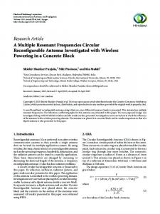
A time-varying magnetic field at a defined area S can be determined with a calibrated circular loop connected to the input of an appropriate measuring receiver (Fig. 5). There may be a passive or an active network between the loop and the output port. The measuring loop can also include a shielding over its circumference against any perturbation of strong and unwanted electric fields. The shielding must be interrupted at a point on the loop circumference. Generally in the far field the streamlines of magnetic flux are uniform, but at near field, in the vicinity of the generator of a magnetic field, they depend on the source and its periphery. Figure 4 shows the streamlines of the electromagnetic vectors generated by the transmitting loop L1. In the near field, the spatial distribution of the magnetic flux B ¼ m0 H over the measuring loop area is not known. Only the normal components of the magnetic flux, averaged over the closed-loop area, can induce a current through the loop conductor. The measuring loop must have a calibration (conversion) factor or set of factors that, at each frequency, expresses the relationship between the field strength impinging on the loop and indication of the measuring receiver. The calibration of a measuring loop requires the generation of a well-defined standard magnetic field on its effective receiving surface. Such a magnetic field is generated by a circular transmitting loop when a defined root-mean-square (RMS) current is passed through its conductor. The unit of the generated or measured magnetic field strength Hav is A/m (amperes per meter) and therefore is also an RMS value. The subscript ‘‘av’’ strictly indicates the average value of the spatial distribution, not the average over a period of T of a periodic function. This statement is important for nearfield calibration and measuring purposes. For far-field measurements the result indicates the RMS value of the magnitude of the uniform field. The traceability of the calibration must be established for the calibration process, through linking the assigned value of any components to the International System of Units (SI). In the following we discuss the requirements for the near-zone calibration of a measuring loop.

∆

CALIBRATION OF A CIRCULAR LOOP ANTENNA*

r2

P

I2 A R () d

E

L1 G

S1

T ds1

A x

r1

0

H +

I y

Figure 1. Configuration of two circular loops.

magnetic field strength Hav in A/m generated by a circular filamentary loop at an axial distance d including the retardation due to the finite propagation time was obtained earlier by Greene [1]. The average value of field strength Hav was derived from the retarded vector potential Aj as a tangential component on the point P of the periphery of loop L2:

Hav ¼

RðjÞ ¼

Ir1 pr2

Z 0

p jbRðjÞ

e

RðjÞ

cosðjÞ dj

qffiffiffiffiffiffiffiffiffiffiffiffiffiffiffiffiffiffiffiffiffiffiffiffiffiffiffiffiffiffiffiffiffiffiffiffiffiffiffiffiffiffiffiffiffiffiffiffiffiffiffiffiffiffiffiffiffi d2 þ r21 þ r22 2r1 r2 cosðjÞ

ð1aÞ

ð1bÞ

In these equations for thin circular loops, I is the transmitting loop RMS current in amperes, d is the distance between the planes of the two coaxial loop antennas in meters, r1 and r2 are filamentary loop radii of transmitting and receiving loops in meters, respectively, b is wavelength constant, b ¼ 2p/l, and l is wavelength in meters. Equations (1) give the exact results for the separation distances even from d ¼ 0. For d ¼ 0 the radii of the loops must be r1ar2, otherwise the integral gives a singularity for j ¼ p, because for r1 ¼ r2 the root in Eq. (1b) being zero. The use of any approximate formula (Eq. 25 in Ref. 1 and Eqs. (2) in Ref. 2) is not suitable, because it imposes restrictions on the range applicability for the approximate equations. Using the expressions of maximum magnetic field Hmax would also not be suitable for purposes of nearfield calibration purpose (see Fig. 2 in Ref. 2). Generally the Eqs. (1) can be determined by numerical integration. To this end we separate the real and imaginary parts of the integrand using Euler’s formula

1. CALCULATION OF STANDARD MAGNETIC FIELDS To generate a standard magnetic field, a transmitting loop L1 is positioned coaxial and plane-parallel at a separation distance d from the loop L2 to be calibrated, as in Fig. 1. The analytical formula for the calculation of the average *This article is based on ‘‘Calibration of Circular Loop Antennas,’’ by Aydin Aykan, which appeared in IEEE Transactions on Instrumentation and Measurement, Vol. 7, No. 2, r 1998 IEEE. 560

CALIBRATION OF A CIRCULAR LOOP ANTENNA

1.5

A I1 ZL Q

Vo

r1 I1

1

E F

I2 = Imax dB

VL

0 I1 = .r1 x

Ix

I1

A VL

0.5

Hav

D

ZL

−0.5 E Z2 = 0

Q

V2 = 0

I2 = Imax

Vo D

Ix

I1

F I

Ix Iav

I2 = Imax Iav

I1 l

561

π.r1

x

0

1

2

5

10 MHz

20

50

100

Figure 3. Deviation of Iav/I1 for a loop radius 0.1 m as 20 log(Iav/I) in decibels versus frequency.

wavelength l and the loop current to be constant in phase around the loop and the loop proper to be sufficiently lossfree. The single-turn thin loop was considered as a circular balanced transmission line fed at points A and D and short-circuited at points E and F (Fig. 2). In an actual calibration setup the loop current I1 is specified at the terminals A and D. The average current was given as a function of input current I1 of the loop [2]:

Figure 2. Current distribution on a circular loop.

Iav ¼ I1

e jj ¼ cos(j) j sin(j) and rewrite Eq. (1a) as Hav ¼

Ir1 ðF jGÞ pr2

ð2aÞ

where Z

p

F¼ 0

Z

p

G¼ 0

cosðbRðjÞÞ cosðjÞ dj RðjÞ

ð2bÞ

sinðbRðjÞÞ cosðjÞ dj RðjÞ

ð2cÞ

and the magnitude of Hav is then obtained as jHav j ¼

Ir1 pffiffiffiffiffiffiffiffiffiffiffiffiffiffiffiffiffi F 2 þ G2 pr2

ð2dÞ

tanðbpr1 Þ bpr1

ð3Þ

The fraction of Iav/I1 from Eq. (3) expressed in decibels gives the conditions for determining of the highest frequency f and the radius of the loop r1. The deviation of this fractions is plotted in Fig. 3. The current I in Eq. (1a) must be substituted with Iav from Eq. (3). Since Eq. (3) is an approximate expression, it is recommended to keep the radius of the transmitting loop small enough for the highest frequency of calibration to minimize the errors. For the dimensioning of the radius of the receiving loop, these conditions are not very important, because the receiving loop is calibrated with an accurately defined standard magnetic field, but the resonance of the loop at higher frequencies must be taken into account. 2.2. Circular Loops with Finite Conductor Radii

It is possible to evaluate the integrals in Eqs. (2) numerically with an appropriate mathematics software on a personal computer. Some mathematics software can directly calculate the complex integral of Eqs. (1). Hence, some of the following equations are written in complex form for convenience. 2. ELECTRICAL PROPERTIES OF CIRCULAR LOOPS 2.1. Current Distribution around a Loop The current distribution around the transmitting loop is not constant in amplitude and in phase. A standing wave of current exists on the circumference of the loop. This current distribution along the loop circumference is discussed by Greene [1, pp. 323–324]. He has assumed the loop circumference 2pr1 to be electrically smaller than the

A measuring loop can be constructed with one or more windings. The form of the loop is chosen as a circle because of the simplicity of the theoretical calculation and calibration. The loop conductor has a finite radius. At high frequencies the loop current flows on the conductor surface and shows the same proximity effect as two parallel, infinitely long cylindrical conductors. Figure 4 shows the cross section of two loops in intentionally exaggerated dimensions. The streamlines of the electric field are orthogonal to the conductor surface of the transmitting loop L1 and they intersect at points A and A0 . The total conductor current is assumed to flow through a fictive thinffi filamenqffiffiffiffiffiffiffiffiffiffiffiffiffiffi tary loop with the radius a1 ¼ r21 c21 , where qffiffiffiffiffiffiffiffiffiffiffiffiffiffiffiffiffiffiffiffiffiffiffiffiffi 2

2

a1 ¼ OA ¼ QP ¼ OQ QP . The streamlines of the magnetic field are orthogonal to the streamlines of electric field. The receiving loop L2 with the finite conductor

562


H

2.3. Impedance of a Circular Loop

Hn

The impedance of a loop can be defined at chosen terminals Q, D as Z ¼ V/I1 (Fig. 2). Using Maxwell’s equation with Faraday’s law curl(E) ¼ joFm, we can write the line integrals of the electric intensity E along the loop conductor through its cross section, along the path joining points D,Q and the load impedance ZL between the terminals Q, A:

Hav

H c2 Br

Ar

Br'

Qr

Or

T

L2

Ar' Qr'

T'

b2

Z

a2 r2

Z

Z

Es ds þ ðAEFDÞ

Es ds þ

Es ds ¼ joFm

ðDQÞ

ð5aÞ

ðQAÞ

h e P L1

Q c1

O

B

Here Fm is the magnetic flux. The impressed emf (electromotive force) V acting along the path joining points D and Q is equal and opposite to the second term of Eq. (5a):

Q'

B' A'

A

Z V¼

Es ds

ð5bÞ

ðDQÞ

b1 a1

The impedance of the loop at the terminals D, Q can be written from Eqs. (5) dividing with I1 as

r1 Figure 4. Filamentary loops of two loops with finite conductor radii and orthogonal streamlines of the electromagnetic vectors, produced from transmitting loop L1.

radius c2 can encircle a part of magnetic field with its effective circular radius b2 ¼ r2 c2. The sum of the normal component of vectors H acting on the effective receive area S2 ¼ pb22 induces a current in the conductor of the receiving loop L2. This current flows through the filamentary loop with the radius a2. The average magnetic field vector Hav is defined as the integral of vectors Hn over effective receiving area S2, divided by S2. The magnetic streamlines, which flow through the conductor and outside of loop L2, cannot induce a current through the conductor along the filamentary loop Ar, Ar0 of L2. The equivalent filamentary loop radii a1, a2 and effective circular surface radii b1, b2 can be seen directly from Fig. 4. The equivalent thin current filament radius a1 of the transmitting loop L1: qffiffiffiffiffiffiffiffiffiffiffiffiffiffiffi a1 ¼ r21 c21

ð4aÞ

The equivalent thin current filament radius a2 of the receiving loop L2 is a2 ¼

qffiffiffiffiffiffiffiffiffiffiffiffiffiffiffi r22 c22

ð4bÞ

The radius b1 of the effective transmitting circular area of the transmitting loop L1 is b 1 ¼ r1 c1

Z¼

V ¼ I1

ð4dÞ

Z

Es ds ðAEFDÞ

þ

I1

Es ds

ðQAÞ

þ

I1

joFm ¼ Zi þ ZL þ Ze I1 ð6Þ

where Zi indicates the internal impedance of the loop conductor. Because of the skin effect, the internal impedance at high frequencies is not resistive. For the calculation of the Zi, we refer to Schelkunoff, [3, p. 263] and Ramo et al. [4, p. 185]. ZL is a known load or a source impedance on Fig. 2. Ze is the external impedance of the loop:

Ze ¼ jo

Fm m Hav S ¼ jo 0 I1 I1

ð7aÞ

We can consider that the loop consists of two coaxial and coplanar filamentary loops (i.e., separation distance d ¼ 0). The radii a1 and b1 are defined in Eqs. (4). The average current Iav flows through the filamentary loop with the radius a1 and generates an average magnetic field strength Hav on the effective circular surface S1 ¼ pb21 of the filamentary loop with the radius b1. From Eqs. (1) and (3) we can rewrite Eq. (7a), for the loop L1:

Ze ¼ j

tanðbpa1 Þ m0 oa1 b1 bpa1

ð4cÞ

The radius b2 of the effective receiving circular area of the receiving loop L2 is b 2 ¼ r2 c2

Z

R0 ðjÞ ¼

Z 0

p jbR0 ðjÞ

e

R0 ðjÞ

cosðjÞdj

qffiffiffiffiffiffiffiffiffiffiffiffiffiffiffiffiffiffiffiffiffiffiffiffiffiffiffiffiffiffiffiffiffiffiffiffiffiffiffiffiffiffiffiffiffiffiffiffi a21 þ b21 2a1 b1 cosðjÞ

ð7bÞ

ð7cÞ

The real and imaginary parts of Ze are the radiation resistance and the external inductance of loops,


respectively: Z p tanðbpa1 Þ sinðbR0 ðjÞÞ m0 oa1 b1 cosðjÞdj ReðZe Þ ¼ bpa1 R0 ðjÞ 0 ð7dÞ ImðZe Þ ¼


Z

p 0

cosðbR0 ðjÞÞ cosðjÞdj ð7eÞ R0 ðjÞ

From Eq. (7e) we obtain the external self-inductance: Le ¼

tanðbpa1 Þ m0 a1 b1 bpa1

Z

p

0

cosðbR0 ðjÞÞ cosðjÞdj R0 ðjÞ

ð7f Þ

563

Arranging Eq. (7b) for Z2e and the current ratio I2/I1 from Eqs. (10), we obtain the external mutual impedance: Z12e ¼ j


Z 0

p jbRd ðjÞ

e

Rd ðjÞ

cosðjÞdj

ð11bÞ

The real part of Z12e may be described as mutual radiation resistance between two loops. The imaginary part of Z12e divided by o gives the mutual inductance M12e ¼

tanðbpa1 Þ m0 a1 b2 bpa1

Z 0

p

cosðbRd ðjÞÞ cosðjÞ dj Rd ðjÞ

ð11cÞ

Equations (7) include the effect of current distribution on the loop with finite conductor radii.

Equations (11b) and (11c) include the effect of current distribution on the loop with finite conductor radii.

2.4. Mutual Impedance between Two Circular Loops

3. DETERMINATION OF THE ANTENNA FACTOR

The mutual impedance Z12 between two loops is defined as

The antenna factor KH is defined as a proportionality constant with necessary conversion of units. KH is the ratio of the average magnetic field strength Hav bounded by the loop to the measured output voltage VL on the input impedance Ri of the measuring receiver.

Z12 ¼

V2 Z2 I2 ¼ I1 I1

ð8Þ

The impedance of Z2 in Eq. (8) can be defined as in Eqs. (6): V2 ¼ Z2i þ ZL þ Z2e Z2 ¼ I2

ð9Þ

here Z2i is the internal impedance, ZL is the load impedance, and Z2e is the external impedance of the second loop L2. The current ratio I2 to I1 in Eq. (8) can be calculated from Eqs. (1), (3), and (4). The current I1 of the transmit loop with separation distance d I1 ¼

tanðbpa1 Þ a1 bpa1

Rd ðjÞ ¼

H pb2 Z av p jbR ðjÞ d e cosðjÞdj 0 Rd ðjÞ

qffiffiffiffiffiffiffiffiffiffiffiffiffiffiffiffiffiffiffiffiffiffiffiffiffiffiffiffiffiffiffiffiffiffiffiffiffiffiffiffiffiffiffiffiffiffiffiffiffiffiffiffiffiffiffiffiffiffiffi d2 þ a21 þ b22 2a1 b2 cosðjÞ

ð10aÞ

tanðbpa2 Þ a2 bpa2

H pb2 Z av p jbR ðjÞ 0 e cosðjÞdj 0 R0 ðjÞ

qffiffiffiffiffiffiffiffiffiffiffiffiffiffiffiffiffiffiffiffiffiffiffiffiffiffiffiffiffiffiffiffiffiffiffiffiffiffiffiffiffiffiffiffiffiffiffiffi R0 ðjÞ ¼ a22 þ b22 2a2 b2 cosðjÞ

ð10bÞ

I2 ¼ Z12i þ Z12L þ Z12e I1

ð12aÞ

Equation (12a) can also be expressed logarithmically: kH ¼ 20 logðKH Þ in dBðA=mÞ . V1

ð12bÞ

For evaluation of the antenna factor there are two methods. The first is by calculation of the loop impedances, and the second is with the well-defined standard magnetic field calibration.

If a measurement loop, (e.g., L2), has a simple geometric shape and a simple connection to a voltage measuring device with a known input impedance Ri, we can determine the antenna factor by calculation. In the case of the unloaded loop from Fig. 2, the open-circuit voltage is

ð10cÞ

V0 ¼ jom0 Hav S2

ð13aÞ

For the case of the loaded loop the current is ð10dÞ

The general mutual impedance between two loops from Eqs. (8) and (9) is Z12 ¼ ðZ2i þ ZL þ Z2e Þ

Hav in ðA=mÞ . V1 VL

3.1. Determination of the Antenna Factor by Computing from the Loop Impedances

and the current I2 of the receive loop for the same Hav (here d ¼ 0) is I2 ¼

KH ¼

ð11aÞ

here Z12i is the mutual internal impedance, Z12L denotes the mutual load impedance, and Z12e is the external mutual impedance.

I¼

V0 V0 ¼ Z RL þ Zi þ Ze

ð13bÞ

The antenna factor from Eq. (12a) can be written with VL ¼ ZLI and Eqs. (13) and (1) as KH ¼

1 Ze Zi 1þ þ in ðA=mÞ . V1 jom0 S2 RL RL

ð14Þ

The effective loop area is S2 ¼ pb22 . The external loop impedance Ze can be calculated with Eqs. (7). The internal

564


The usable highest frequency of the loop L1 decreases with the additional electrical length of the twisted-pair line. This consideration is used to define an appropriate length of the twisted-pair transmission line. The antenna factor in Eqs. (12) can be fully defined for each frequency through the measurement of the transmitting loop current I1 at the interface M0 and voltage VL at the interface F:

impedance Zi is in general small in respect to external impedance Ze, and can be neglected. For a more precise calculation of the internal impedance Zi due to the skin effect, refer to Refs. 3 and 4. 3.2. Standard Magnetic Field Method In the calibration setup in Fig. 5 we measure the voltages with standard laboratory measuring instrumentation with the 50 O interface impedances. The device to be calibrated consists at least of a loop and a cable with an output connector. The measuring loop can also include a passive or active network between the terminals C, D and a coaxial shield on the circular loop conductor against unwanted electric fields, depending on its development and construction. The impedance ZCD and the voltage VCD at the terminals C,D is not accurately measurable. The behavior of the attenuation and/or the gain between the interfaces D,C and F cannot be accurately defined. Such a complex measuring loop must be calibrated with the standard magnetic field method through the calibration setup in Fig. 5. To prevent the deterioration of the magnetic field, produced by L1, we must place the attenuators sufficiently far from the transmitting loop using a twistedpair balanced line. The attenuators (e.g., nominal 10 dB) must have the calibrated attenuations m for attenuator 1 and n for attenuator 2, and the calibrated interface resistances (nominal 50 O). The shielding of the attenuators must be electrically connected at the points x. The ferrite pads on the twisted-pair line and on the coaxial cable attenuate the magnetic field scattering from the measuring transmission lines. The electrical length Le of the twisted transmission line must be taken into account and the equation (3) must be redefined for the average current Iav: Iav ¼ I1

tanðbðpa1 þ LeÞÞ bðpa1 þ LeÞ

Z p jbRd ðjÞ I1 tanðbðpa1 þ LeÞÞ a1 e cosðjÞdj pb2 0 Rd ðjÞ pa1 þ Le KH ¼ ð16aÞ VL Here r1 ¼ a1, r2 ¼ b2, Le is the electrical length of the twisted-pair transmission line and Rd defined with Eq. (10b). Attenuator 1 attenuates the current I1 with the ratio m and hence the current through the interface M0 becomes we m . I1. The transmitting loop current is I1 ¼ V2/m R2. Consequently, the current flowing through the interface N0 is I1/(n . m). With the measuring receiver we can measure first the voltage V2 at the interface M0 to obtain the transmitting loop current I1, which produces the magnetic field Hav in the receiving loop L2. We then measure the voltage VL at the interface F, which is produced by the same magnetic field Hav. With setting a ¼ V2/VL, we can write Eq. (16a) as Z p jbRd ðjÞ a tanðbðpa1 þ LeÞÞ a1 e cosðjÞ dj ð16bÞ KH ¼ m R2 ðbpa1 þ LeÞ pb2 0 Rd ðjÞ Equation (16b) is expressed in SI units [(A/m)V 1] and can also be expressed logarithmically as

ð15Þ

kH ¼ 20 logðKH Þ in dB½ðA=mÞ . V1 Hav

1. Step: Terminator 2. Step: Receiver

Network D

VL

Ri

VCD

F

I2

ZCD

r2

C

Measuring loop L2 d

1. Step: Receiver 2. Step: Terminator V2 R2

M'

m·I1

Attennuator 1 m M x

Generator Q

R1

V0

V1

N N'

B r1

2 n x

I1/n·m

Le

A Transmitter loop L1

Figure 5. Calibration setup for circular loop antennas.

I1

ð16cÞ

CAPACITANCE EXTRACTION

The ratio of the measured voltages is an attenuation and with an appropriate measuring setup the calibration is realized as an attenuation measurement. A network analyzer is generally used for this purpose instead of discrete measurements at each individual frequency with a signal generator and a measuring receiver. A network analyzer can normalize the frequency characteristic of the transmit loop current I1 and gives a quick overview of the measured attenuation for the frequency band under consideration. Equation (16b) reduces the calibration process of the loop to an accurate measurement of attenuation a for each frequency. The other terms of Eq. (16a) can be calculated depending on the geometric configuration of the calibration setup at the working frequency band of the measuring loop. The calibration uncertainties are also calculable with the given expressions. The uncertainty of the separation distance d between two loops must be taken into consideration as well. At a separation distance doa1, the change in the magnetic field is high (see Fig. 2 in Ref. 2). For a calibration setup the separation distance d can be defined as small as possible. However, the effect of the mutual impedance must be taken into account in the calibration process, and a condition for definition of the separation distance d must be given (Fig. 5). If the second loop is open-circuited, that is, if the current I2 ¼ 0, the current I1 is defined only from the impedances of the transmitting loop L1. In the case of a short-circuited second loop L2, I2 is maximum and the value of I1 will change depending on the supply circuit and loading of the transmitting loop. A current ratio q between these two cases can be defined as the condition of the separation distance d between the two loops. It is assumed that the generator voltage V0 is constant. The measuring loop L2 is terminated by ZL. For ZL ¼ 0 and VCD ¼ 0, one obtains the current I1 in the transmitting loop as I1ðZL ¼ 0Þ ¼

V0 Z2 R1 þ R2 þ ZAB 12 ZCD

ð17aÞ

V0 R1 þ R2 þ ZAB

All equations in this article are written in their original exact form without approximations, which usually restrict their range of validity in applications regarding frequency range, distance, and other quantities. Also, no simplifications of the equations are made. All equations deliver the results directly in units of SI with an appropriate mathematical software on a personal computer. The electrical properties of the loops are calculable without approximation. The necessary conditions are given for the choice of dimensions of the measuring and transmitting circular loops and the separation distance d. For calibration of circular loop antennas, the standard magnetic field method is recommended with the calibration setup in Fig. 5 and also for determination of the antenna factor KH and kH in Eqs. (16b) and (16c). The calibration process is based on the measurement of attenuation at each frequency on the same impedance level of 50 O, using the standard laboratory equipment. The measurement can also be accelerated by using a network analyzer. BIBLIOGRAPHY 1. F. M. Greene, The near-zone magnetic field of a small circularloop antenna, J. Rese. Natl. Bur. Stand. Eng. Instrum. 71C(4): 319–326 (Oct.–Dec., 1967). 2. A. Aykan, Calibration of circular loop antennas, IEEE Trans. Instrum. Meas. 47(2): 446–452 (April 1998). 3. S. A. Schelkunoff, Electromagnetic Waves, Van Nostrand, New York, 1943.


I1ðZL ¼ 0Þ R þ R þ Z 1 2 AB ¼ q 2 I1ðZL ¼ 1Þ Z12 R þ R þ Z 1 1 2 AB ZAB ZCD

q ¼

4. CONCLUSION

ð17bÞ

The ratio of Eq. (17a) to Eq. (17b) is

here with the coupling factor k ¼ Z12 = two loops:

The influence of the loading of the second loop on the transmitting loop can also be found experimentally. The change of voltage V2 at R2 in Fig. 5 must be considerably small (e.g., o0.05 dB) when the measuring loop is shortcircuited at the chosen separation distance d.

4. S. Ramo, J. R. Whinnery, and T. van Duser, Fields and Waves in Communication Electronics, 3rd ed., Wiley, New York, 1994.

and for ZL ¼ N, that is, I2 ¼ 0 I1ðZL ¼ 1Þ ¼

565

ð18aÞ

pffiffiffiffiffiffiffiffiffiffiffiffiffiffiffiffiffi ZAB ZCD between

R1 þ R2 þ ZAB 2 R1 þ R2 þ ZAB ð1 k Þ

WENJIAN YU ZEYI WANG

ð18bÞ

where R1 ¼ R2 ¼ 50 O and ZAB, ZCD, and Z12 can be calculated from Eqs. (7) and (11). For greater accuracy one must try to keep the ratio q close to unity (e.g., q ¼ 1.001).

Tsinghua University Beijing, China

1. INTRODUCTION Since the early 1950s, microwave circuits have evolved from discrete circuits to planar integrated circuits, then to multilayered and three-dimensional integrated circuits. With the increased circuit density, the multiconductor line in multilayered dielectric media has become the major form of the transmission line or interconnect. Multilayered routing reduces the area as well as the volume of the

566


circuit. However, as a result, electromagnetic coupling among conductors greatly influences circuit performance. In some microwave integrated circuits, this coupling effect is utilized to construct compact circuit components. But under most circumstances, it is regarded as a parasitic effect that must be modeled accurately for verification of the circuit’s validity and performance. In the related field of very-large-scale integration (VLSI) circuits, electromagnetic coupling among interconnects is also becoming increasingly important. With the introduction of deep-sub-micrometer (DSM) semiconductor technologies, the on-chip interconnect wire can no longer be considered equipotential jointing. The parasitic effects introduced by the wires display a scaling behavior that differs from that of active devices such as transistors, and these effects tend to gain importance as device dimensions are reduced and circuit speed is increased. In fact, they begin to dominate some of the relevant metrics of digital integrated circuits such as speed, energy consumption, and reliability. A typical recursive design flowchart of a state-of-the-art integrated circuit (IC) is shown in Fig. 1, where a postlayout step termed parasitic extraction precedes gate-level simulation. The task of parasitic extraction is to model the electromagnetic effects of the wire with parasitic components of capacitance, resistance, and inductance, so that a more accurate circuit simulation can be performed. With the increase in working frequency and development of silicon technologies, the discrepancy between the microwave IC and the common VLSI circuit becomes marginal. Therefore, the electromagnetic modeling and accurate extraction of the interconnect parasitics have become a subject of advanced research in both fields to date. Among the three parasitic parameters, capacitance has attracted the most attention because it greatly influences time delay, power consumption, and the signal integrity and its calculation becomes complicated under DSM technologies. In the following sections, the fundamental theory and contemporary methodology and algorithms of capacitance extraction will be discussed.

Function Spec.

Front-end

RTL

Behavior Simul.

Logic Synth.

Stat. Wire Model

Gate-level Net.

Gate-level Simul.

2. PROBLEM FORMULATION As is well known, the capacitor is a commonly used component in electric or electronic equipment. It is usually composed of two conductors insulated from each other. When charged, the two surfaces of the conductor facing each other carry equal and opposite charges Q and Q, respectively (see Fig. 2). The electric potential difference between the two conductors f1–f2 is called the voltage of the capacitor and is always denoted by V. Experiments and theoretical analyses show that, for a capacitor, Q is always proportional to V and thus the ratio Q/V is a constant determined by the structure of the capacitor. This ratio is called the capacitance of the capacitor and is denoted by C: C ¼ (Q/V). In the International System of Units (SI), the unit of capacitance is the faraday (F). It expresses the capacitance of a capacitor that has one coulomb on one of its poles when the potential difference is 1 V. Other commonly used units of capacitance are mF (10 6 F), pF (10 12 F), and f F (10 15 F). The capacitance of some simple capacitor can be calculated easily. For example, for the parallel-plate capacitor shown in Fig. 2, we have C¼

e0 ¼

1 ¼ 8:85 1012 C2 =N . m2 4p 9 109

where er is the relative permittivity of the insulating material, S is the area of the plate, and d is the distance between two parallel plates. Specific capacitors widely used in the design of microwave circuits include the interdigital capacitor and the metal–insulator–metal (MIM) capacitor. Figure 3 shows the physical layout of an interdigital capacitor with nine fingers, and Fig. 4 shows the cross-sectional view of an MIM capacitor with the GaAs process. The interdigital capacitor works with the electrostatic coupling between the intercrossed fingers, and has a very high Q value. So, it is widely used in the high-frequency microwave circuits.

1

Floorplanning Parasitic Extraction Place & Route

ð1Þ

where e0 is the dielectric constant of free space and in SI, is expressed as

+Q

d Back-end

e0 er S d

r S

2

−Q

Layout Figure 1. A typical flowchart of IC design.

Figure 2. A parallel-plate capacitor.


567

Master conductor, IV Neumann boundary

z 15.00

Figure 3. An interdigital capacitor.

30

30.00

The MIM capacitor has simple geometry and is easily fabricated, and its capacitance is controlled by the dimensions of the polar planes. Since the interdigital capacitor and the MIM capacitor are widely used, calculation of the parameters of their structures within given the working frequency and corresponding capacitor value becomes an important issue for both design and optimization. This can be regarded as the reverse procedure of capacitance extraction. For further discussion of this issue, please refer to the literature [39,40]. Actually, the capacitor has more generalized forms than that described above, which consists of two insulated conductors. The capacitance of a single conductor (conductor 1) is defined as if another conductor (conductor 2) were located at an infinite distance away to form a joint capacitor (conductors 1 þ 2). For example, the capacitance of an isolated conductor sphere with radius of R can be calculated as C ¼ 4pe0 R. Many conductor interconnect wires are involved in the microwave IC and the common VLSI circuit, and they are insulated by some dielectric such as oxide SiO2. The capacitance between any two wires reflects the electrostatic coupling effect between these wires, and calculating these capacitances with high accuracy is very important for analysis of the circuit’s performance. For an N-conductor system, such as the interconnect wires in an IC, an N N capacitance matrix [Cij]N N is defined by

Grounded substrate

3.00

Figure 5. A structure involving 2 2 crossover interconnect wires.

conductor i, and Uj is the electric potential of conductor j (usually the known bias voltage). Figure 5 shows a typical crossover wires in the VLSI system, where the coupling capacitances between any two conductors need to be calculated. Accurate modeling of the wire capacitances in a stateof-the-art integrated circuit is not a trivial task. It is further complicated by the fact that the interconnect structure of contemporary integrated circuits is threedimensional (see Fig. 5). The capacitance of such a wire is a function of its shape, environment, distance from the substrate, and distance to surrounding wires. Generally SiO2 is the insulating material among interconnect wires in integrated circuits, although some materials with lower permittivity, and thus lower capacitance, are coming into use. The relative permittivity er of several dielectrics commonly used in integrated circuits is presented in Table 1. It should also be pointed out that er of air or vacuum is 1.

3. METHODOLOGY AND ALGORITHMS Qi ¼

N X

Cij Uj ;

i ¼ 1; 2; . . . N;

ð2Þ

j¼1

where Cij (iaj) is the coupling capacitance between conductors i and j, and Cii is the self-capacitance or total capacitance of conductor i. Qi is the induced charge on

With the advances in IC technology, the methodology of capacitance extraction has evolved from one-dimensional (1D), two-dimensional (2D), 2.5-dimensional (2.5D), to three-dimensional (3D) to meet the required accuracy. In this section, the 1D and 2D methods are briefly introduced. Then, the 2.5-D method and the mechanism of the modern commercial capacitance extraction tools that employ the 3D capacitance extractor are presented. Finally, we will discuss some details of algorithms of the 3D field solver for capacitance extraction. 3.1. 1D and 2D Methods

SiN

SiO2

GaAs

Figure 4. An MIM capacitor (cross-sectional view).

From the formula for calculation of parallel-plate capacitance [Eq. (1)], we can infer that the capacitance is proportional to the overlapping area between the conductors and inversely proportional to their separation distance. This is very important for capacitance extraction without a high degree of precision.

568


Table 1. Relative Permittivity of Several Commonly used Dielectric Materials Dielectric Material Relative permittivity (er)

Silicon

Alumina (Package)

Silicon Nitride (Si3N4)

Glassepoxy (PCB)

Silicon Dioxide

Polyimides (Organic)

Aerogels

11.7

9.5

7.5

5

3.9

3–4

B1.5

Figure 6 shows a typical microstrip structure, where there is only a single rectangular conductor over a ground plane. This structure is very different from the above parallel-plate model discussed because of the existence of the capacitance between the sidewalls of the wire and the substrate, called the fringing capacitance. To avoid the time-consuming numerical modeling of this geometry, an approximate 1D method can be used as a good engineering practice. The capacitance is assumed to be the sum of two components: (1) a parallel-plate capacitance determined by the vertical field between a wire of width w and the ground plane and (2) the fringing capacitance modeled by a cylindrical wire with radius equal to the conductor thickness H. So, this simple and practical 1D formula becomes C ¼ Carea þ Cfringe ¼

e.w 2pe þ d log ðd=HÞ

where w ¼ W H/2 is a good approximation for the width of the parallel-plate capacitor (W is the width of the wire), d is the distance between the ground plane and the bottom of wire, and e is the permittivity of the insulating material. With this formula, we obtain the approximate capacitance per unit length. In another kind of 1D capacitance extraction, the area and perimeter parameters of interconnect geometries are first obtained. Then, a fine-tuned set of area and perimeter weights per routing layer can be used to calculate capacitance values as an inner product [1]: C ¼ ðarea amount; perimeter amountÞ . ðarea weight; perimeter weightÞ Such area and perimeter weights can be obtained by precharacterization of an ‘‘average’’ environment of a wire. The area can be that from single layer or a combination of layer overlaps. Usually, the 1D extraction method works well when the number of interconnect layers is restricted to only one or two. However, the current process technology often involves many more interconnect layers, and they are also of high density. So, several capacitance components of a wire embedded in the multilayered interconnect system may

exist, other than the only capacitive coupling to the ground plane (see Fig. 7). Each wire is coupled not only to the grounded substrate but also to the neighboring wires on the same layer and on adjacent layers. Not all capacitive components terminate at the grounded substrate; actually a large number of them connect to other wires. These (fringing, lateral, parallel, etc.) capacitors between wires not only form a source of noise (crosstalk among signal lines) but also can have a negative impact on the circuit performance. To model the capacitance in the multilayered interconnect system with higher accuracy, 2D capacitance extraction methodology was developed. In 2D capacitance extraction, accurate geometry modeling and numerical techniques are implemented for the cross section of simulated structure (as in Fig. 7). For the 2D region of dielectrics, the electric field equation is solved with numerical techniques. 2D extraction ignores all three dimensional details and assumes that the geometries being modeled are uniform in one dimension, usually the signal propagation direction. Therefore, 2D capacitance extraction is only suitable only for some special cases, such as like the transmission line. The details of numerical techniques for solving the electric field will be introduced in Section 3.3, albeit in a 3D manner. 3.2. 2.5D Method and Commercial Capacitance Extraction Tool The 2.5D (also called quasi-3D) method goes a step further than 2D extraction. Its main idea is to calculate the capacitance of several cross sections (using the 2D method) and combine the 2-D results into the final capacitance value. A typical 2.5D capacitance extraction method is also called the ‘‘(2 2)D method’’, in which any 3D structure is swept in two perpendicular directions and by considering the geometry overlapping, 3D structure can be modeled more accurately (see Fig. 8). In Fig. 8, an m2 wire crosses an m1 wire. Along direction A, a 2D cross-sectional view is shown in the middle. Along direction B, the other 2D cross section is shown to

Fringing

Parallel Lateral

Cfringe

Carea Ground Figure 6. A conductor above a ground plane (cross-sectional view).

Substrate Figure 7. Capacitive coupling between wires in a multilayered interconnect system.


A

569

Conformal dielectric

w2 B

C1f1 C C1f 2 1o

w1

C2f1 C2o C2f 2

m1 m2

Top view

Cross section view A

Cross section view B

Figure 8. 2.5D capacitance for a crossover structure.

the right. Solving the two orthogonal strictly 2D problems numerically, we obtain CA ¼ C1f1 þ C10 þ C1f2, CB ¼ C2f1 þ C20 þ C2f2 (see Fig. 8). Then, Cm1,m2 ¼ CA w1 þ (CB C20) w2, where w1, w2 are the widths of wires m1 and m2, respectively. However, this method is still not very accurate. The error could be more than 10%, especially for coupling capacitance, which is very important for signal integrity analysis. Obviously, true 3D extraction is a straightforward method to achieve high precision. However, the 3D electrostatic Laplace equation must be solved numerically within a complicated 3D structure. This consumes extensive computational effort. 3D capacitance extraction (usually called the ‘‘field solver’’) is actually not a trivial extension of the 2D case. This aspect is discussed further in Section 3.3. For the current task of capacitance extraction in modern IC design, using the 3D extraction method directly is impossible because of its huge expense of memory and CPU time. To obtain a good tradeoff between accuracy and efficiency, modern capacitance extraction tools utilize special techniques for the full-chip extraction task, which is usually divided into three major steps [1]: 1. Technology Precharacterization. Given a description of the process cross sections, tens of thousands of test structures are enumerated and simulated with 2D and/or 3D field solvers. These structures are of medium dimensions. The resulting data are collected either to fit some empirical formulas or to build lookup tables (either type is called a ‘‘pattern library’’). In Ref. 3, analytical equations are used for model fitting. A good fit would require fewer simulation points. The number of patterns can be reduced by pattern reduction techniques. Arora et al. [4] present a pattern compression technique that reduces the total number of precharacterizaiton patterns. With this technology, the capacitance in some layout pattern can be extrapolated from the capacitance values in two simpler precharacterization patterns, without losing much accuracy. Capacitance field solvers employ different numerical algorithms, and they may give different answers for certain special layout structures depending on the problem setup and boundary conditions. Therefore, the precharacterizaiton software should have the flexibility to incorporate any third-party field solvers. This first step should be performed only

Figure 9. A realistic vertical cross section of IC interconnect. We see that conductors on layers 1–5 are trapezoidal, and there is a conformal dielectric on top of the top layer metal (passivation). (SEM photograph courtesy of IBM Corp. r Copyright IBM Corp. 1994, 1996.)

once per process technology. The challenge in this area includes the handling of increasingly complex processing technology, such as low-k dielectric, airbubble dielectric, nonvertical conductor cross sections, conformal dielectric (see Fig. 9), and shallow trench isolations. 2. Geometric Parameter Extraction. This is also an integral part of precharacterization. If a geometric pattern requires 10 parameters to describe, there is a corresponding precharacterization of 1 510 (B10,000,000) patterns to simulate. This is assuming that five sample points are taken in each of the 10 parameters, resulting in a 10-dimensional (10D) table of the dimensions given above. This is clearly not feasible. On the other hand, if a geometric pattern can be described by very few parameters, then it is difficult for it to be accurate. In a full-chip situation, the runtime of geometric parameter extraction can be very time/space-consuming, with millions of interconnect polygons to analyze. Time/ space-efficient geometric processing algorithms are very important. Habitz and Wemple [5] present a geometric parameter reduction technique in which geometric parameters can be dramatically reduced by taking advantage of the shielding effect. Conductors two layers away from the main conductor of interest do not require a precise description. This is particularly useful for the very-deep-sub-micrometer geometry, where a very distant conductor mesh behaves like a large airplane. 3. Calculation of Capacitance from Geometric Parameters. Here, the geometric parameters are matched to some entries in the pattern library. Usually a fullchip or full-path extraction task involves at least thousands of conductors. The whole structure is chopped into medium-size pieces first, which are then calculated with the pattern-matching approach described above. Finally, the capacitance values must be combined to get the desired result.

570


One major source of error is called the pattern mismatch, where extracted geometry parameters do not have an exact match in the pattern library. At this time, there are two remedies to perform the capacitance calculations. One method is to enhance the pattern library by running field solvers at the full-chip extraction time. The other method is to employ heuristics to synthesize a solution from closely matched precharacterization patterns. Even if all the geometric patterns match the library completely, there could still be discontinuities in the layout pattern decomposition, which is another source of error. This error is analyzed in Ref. 6, where the error bound was obtained by utilizing the ‘‘empty’’ and ‘‘full’’ boundary conditions.

ð3Þ

should be pointed out that the infinite-domain model is ideal for simulating isolated structures, but for the on-chip application it is not accurate because of the influence of neighboring conductors. On the other hand, the finitedomain model considers a part cut from actual layout of VLSI circuit; it is suitable for the realistic capacitance extraction of VLSI interconnects [8]. Now, both models of capacitance extraction are used in different applications, and accordingly the numerical methods are also different. The problems a numerical algorithm usually encountered in modeling are discussed below. Classifications of the 3D field solver methods include the domain discretization method, the boundary integral equation method, semianalytical approaches, and the stochastic method. The domain discretization method includes the finite-difference method (FDM) [10], finiteelement method (FEM) [11], and the method of the measured equation of invariance (MEI) [13,14]. The boundary integral equation method includes the method of moment [15], indirect boundary element method (BEM) [8,17–27], and direct boundary element method [28–34]. The semianalytical approaches combine the analytical formulas and some traditional numerical methods [9,35–37]. The stochastic method is based on statistical theory [38]. FDM and FEM discretize the entire 3D domain, thus producing a linear algebra system with large order; hence the computational speed of these methods is greatly limited. However, since both methods are relatively well established, they are still used in the industry as a reference tool with accurate values calculated under fine grids. For example, the famous software of 2/3D capacitance extraction ‘‘Raphael’’ utilizes FDM, and the ‘‘SpiceLink’’ of Ansoft Corp. is based on FEM. Since the mid-1990s, the boundary integral equation method has begun to replace the domain discretization method because of its high performance. In both indirect and direct BEM, only the boundary of 3D domain is discretized, and a smaller system of linear equations is obtained. Problems encountered with the complex boundary can be effectively handled with BEM, whose accuracy is superior to that of FEM as well. Thus, the BEM with rapid computating techniques has become the focus of research on the 3D field solver.

where u is the electric potential. This equation can be transformed into different mathematical formulations. Then, various numerical methods are employed to solve it with different levels of efficiency. According to the domain of the above Laplace equation (3), there are two models for capacitance extraction: (1) the infinite-domain model, in which the electrostatic field spreads to the infinite, resulting in an infinite problem space; and (2) the finite-domain model, where the electrostatic field is restricted within a finite domain, with the Neumann condition on the outer boundary [8]: ð@u=@nÞ ¼ 0. This means that electric field is not able to spread out of the finite problem domain. The Neumann condition is also called the reflective boundary condition, and is introduced as the ‘‘magnetic wall’’ in Ref. 9. It

3.3.2. Indirect Boundary-Element Method. The indirect boundary method can be regarded as a variation of the method of moments (MoM). Because only the domain boundary needs to be discretized, the indirect BEM involves much fewer unknowns than does FDM or FEM. However, it leads to a dense coefficient matrix, whose formation and solution introduce many difficulties. The innovation of the multipole acceleration method, the singular-value decomposition (SVD) method, and the hierarchical method has made the indirect BEM more applicable. Now, indirect BEM combined with a fast computational technique has become a main choice for the 3D field solver. The indirect BEM method is also called the equivalent charge method, whose boundary integral equation involves the surface charge density sðx0 Þ as an unknown

3.3. Algorithms for 3D Field Solver The 3D method can be used model the actual geometry accurately, so it behaves with the highest precision. 3D capacitance extraction becomes increasingly important under the DSM technology of VLSI circuit, although presently it is used widely only as a library-building tool in the industry. More recently, much research work has been devoted to improve the efficiency of the 3D extraction method. Related papers are published on the annually held conferences (Design Automation Conf., Int. Conf. Computer-Aided Design, etc.) and many academic journals (IEEE Trans. Microwave Theory Tech., IEEE Trans. Comput. Aided Design, etc.). To date, some 3D extraction algorithms have been developed to integrate with the commercial software of some electronic design automation (EDA) companies in the Silicon Valley (in California). Research on 3D capacitance extraction is still advancing very rapidly. In this section, the principles and mainstream techniques of the 3D field solver are introduced. More cuttingedge techniques are mentioned with related references. 3.3.1. Overview. For a system involving multiple conductors (see Fig. 5), with one conductor setting 1 V and others 0 V, the electrostatic equation (called the Laplace equation) need to be solved with a homogenous dielectric region [7]: r2 u ¼

@2 u @2 u @2 u þ 2 þ 2 ¼0 @x2 @y @z


function Z uðxÞ ¼

Gðx; x0 Þsðx0 Þda0 ðx 2 GÞ

ð4Þ

G

where Gðx; x0 Þ is Green’s function. For free space, Gðx; x0 Þ ¼ 1=jjx x0 jj; G is the boundary surface. After solving the surface charge density sðx0 Þ, the charge on conductor i can be calculated with Qi ¼

Z

sðx0 Þda0

ð5Þ

Sd ðiÞ

where Sd(i) is the surface of conductor i. We discretize the surfaces of m conductors into n constant elements (or panels); then the potential at the center of the kth panel xk can be expressed as a sum of the contributions of all the panels uk ¼

n Z X j¼1

sj ðx0 Þ da0 0 Gj kx xk k

where sj ðx0 Þ is the surface charge density of panel j (Gj ). Substituting the known boundary conditions, we obtain a dense linear algebra equation. Pq ¼ b

ð6Þ

where the coefficient matrix P is dense and nonsymmetric. The Krylov subspace iterative method, such as the generalized minimal residual algorithm (GMRES) [2], is usually used to solve this equation. For a problem involving multiple dielectrics, the polarization charge density on the dielectric interface needs to be introduced, which contributes to the potential distribution together with the free charge density on conductor surfaces. Therefore, the problem becomes equivalent to that in the free space and the simple free-space Green function is used to form Eq. (4). Except for Eq. (4) on each conductor panel, the normal derivative of the potential satisfies ea

@u þ ðxÞ @u ðxÞ ¼ eb @na @na

ð7Þ

with xAinterface of ea and eb at any point x on a dielectric interface. Here na is the normal to the dielectric interface at x that points into dielectric a and ea and eb are the permittivities of the corresponding homogenous dielectric region; u þ (x) is the potential at x approached from the side of the interface ea , and u (x) is the analogous potential for the b side. For the multidielectric problem, the so-called totalcharge Green function approach presented above involves more unknowns at the interfaces. Another choice to deal with the problem is to employ the multilayered Green function. Then, only the free charge density on the conductor surfaces needs to be considered as an unknown function. However, to evaluate the Green function for the multilayered medium, infinite summations are involved,

571

which is very time-consuming. Oh et al. [20] derived a closed-form expression of Green’s function for the multilayered medium by approximating the Green function using a finite number of images in the spectral domain. This greatly reduces the computational task. Li et al. [22] presented for the first time the general analytical formulas for the static Green functions for shielded and open arbitrarily multilayered media. Zhao et al. [21] an efficient scheme for the generation of multilayered Green functions using a generalized image method presented. The multilayered Green function is much more complicated than the free-space Green function; it is applicable only to the simple stratified structure of multiple dielectrics, while for more complex structures, such as the conformal dielectric, the deduction of Green’s function may be impossible. More research work has been undertaken to accelerate the capacitance extraction using the total-charge Green’s function approach. In 1991, Nabors et al. applied the multipole accelerated (MPA) method successfully, proposed earlier by Greengard and Rokhlin [16], to 3D capacitance extraction with the indirect BEM. In the MPA method, calculation of the interaction between charges [i.e., the coefficients in (6)] is divided into two parts: the near-field computation and the far-field computation. For the near-field computation, the coefficients are calculated directly; for the far-field computation, the multipole expansion and local expansion are used to expedite the computation. Therefore, the CPU time of forming and solving (6) with the iterative equation solver is greatly reduced. Figure 10 illustrates of the multipole expansion. Nabors and White [18], developed the adaptive, preconditioned MPA method. The corresponding software prototype FastCap is shared on the MIT Website, and has become a popular tool of capacitance extraction for relevant researchers. To date, the capacitance extraction using the MPA indirect BEM is still undergoing research [25]. In 1998, a fast hierarchical algorithm for 3D capacitance extraction was proposed at the Design Automation Conference, and was reprinted in a journal article [24]. Similar to the multipole algorithm, it is also based on fast computation of the ‘‘N-body’’ problem. For the singular integral kernel of 1=jjx x0 jj, it can achieve high acceleration of computation, and only O(N) operations are needed

n2 charge points R i

r

ri

n1 evaluation points Figure 10. Evaluation point potentials are approximated with a multipole expansion [17].

572


for each iteration. For other weaker-singular kernels, the efficiency of this method may be reduced. In 1997, Kapur et al. and Long [19] proposed an accelerated method based on the singular-value decomposition (SVD) method that is independent of the kernel and based on the Galerkin method using the pulse function as the basis function. It requires an O(N) times operation to construct the coefficient matrix and O(N log N) operations to perform an iteration. The precorrected fast Fourier transform (FFT) algorithm [23] has the same computational complexity, while it is based on the collocation method for discretization. These studies on capacitance extraction with indirect BEM all handle the infinite-domain model. In 1996, Wang et al. [8] improved the multipole accelerated indirect BEM, enabling it to handle the finite-domain problem and also proposed a parallel multipole accelerated 3D capacitance simulation method based on nonuniformed cube partition. Other fast computational methods for indirect BEM include those based on wavelets [26] and the multiscale method [27]. 3.3.3. Direct Boundary-Element Method. The direct BEM is based on the direct boundary integral equation (BIE), and is suitable for solving the 3D Laplace equation with varied boundary conditions [12]. However, the direct BEM method is generally used to deal with the finite-domain model of capacitance extraction. Within the finite domain that is involved in capacitance extraction (see Fig. 11), the electric potential u satisfies the following Laplace equation with mixed boundary conditions [32] 8 e r2 u ¼ 0; > > < i u ¼ u0 ; > > : q ¼ @u=@n ¼ q0 ¼ 0;

in Oi ði ¼ 1; . . . ; MÞ on Gu

ð8Þ

on Gq M

where the whole domain O ¼ [ Oi , where Oi stands for the space possessed by the ith dielectric. Gu represents the Dirichlet boundary (conductor surfaces), where u is known as the bias voltages; Gq represents the Neumann boundary (outer boundary of the simulated region), where the electric flux q is supposed to be zero. Here n denotes the unit vector outward normal to the boundary. At the dielectric interface, the compatibility equation (7) holds. With the fundamental solution as the weighting function, the Laplace equations in (8) are transformed into the

Conductor

Neumann boundary

3 2 1 Substrate Figure 11. A structure with three dielectrics (cross-sectional view).

following direct BIEs by the Green identity [12] cs uis þ

Z

q ui dG ¼ @Oi

Z

u qi dG ði ¼ 1; . . . ; MÞ @Oi

where uis is the electric potential at collocation point s (in dielectric region i) and cs is a constant dependent on the boundary geometry near to the point s. u ¼ 1=4pr is the fundamental solution of the 3D Laplace equation, whose derivative along the outward normal direction n is q ¼ @u =@n ¼ ðr; nÞ=4pr3 , r is the distance from the collocation point to the point on G, and qOi is the boundary that surrounds dielectric region i. Employing the collocation method after discretizing the boundary, such as that in the indirect BEM, we obtain system of linear equations [32]: Ax ¼ f

ð9Þ

Finally, with the preconditioned Krylov iterative equation solver, such as the GMRES algorithm [2], the normal electric field intensity on the conductor surface is obtained [32]. In direct BEM, variables of both potential and field intensity are involved; thus two kinds of integral kernels are found. Although this is more complex than the indirect BEM method, direct BEM has its own advantages: (1) it is suitable for capacitance extraction within the finite domain since two variables are included, and (2) because the variables in each BIE are within the same dielectric region, it has a ‘‘localization’’ characteristic, which leads to a sparse linear system for problem with multiple dielectrics. In direct BEM, a great deal of time and memory are consumed in forming and solving the system of discretized BEM equations. Wang et al. continued the research work of Fukuda [28] on 2D capacitance extraction using direct BEM, extending it to the 3D structure of VLSI interconnects [32]. An efficient analytical/semianalytical integration scheme was used to accurately calculate the boundary integrals under the VLSI planar process. This method achieves high computational speed and accuracy when forming Eq. (9) [32]. In 1996, Bachtold et al. [29] extended the multipole method to handle the ‘‘potential boundary integral’’ (whose kernel is 1/r3) in the direct BEM. They discussed the model of multiple dielectrics within the infinite domain. In 1999, Gu et al. extended the fast hierarchical method used in the indirect BEM and made it feasible to apply it for direct-BEM-based capacitance extraction [30]. In 2000, Yu et al. proposed a quasi-multiple medium (QMM) method, based on the localization characteristic of direct BEM [32]. The QMM method exploits the sparsity of the resulting coefficient matrix when handling the multidielectric problem. Together with the efficient equation organization and iterative solving technology, the QMM accelerated method has greatly reduced the computing time and memory usage. Figure 12 shows that a typical 3D interconnect capacitor with five dielectric layers is cut into 5 3 2 fictitious medium regions. The QMM method has been successfully applied to actual 3D multidielectric


Neumann boundaries, where electrical flux is 0

573

y z

Dielectric layers

z

x y

x Master conductor, 1 V (Other conductors are with 0V)

Figure 12. A typical 3D interconnect capacitor with five dielectric layers is cut into 3 2 structure.

capacitance extraction [32,34]. For the finite-domain multidielectric problem, the QMM-based method has shown a 10 higher computation speed and memory saving over the multipole approach (FastCap 2.0) with comparable accuracy [34]. Another kind of field solver, called the ‘‘global approach,’’ does not solve the resulting linear system in the usual way. The global approach discretizes the field equations and converts them to a circuit network of resistors or capacitors. Finally, with circuit reduction or matrix computation, the whole resistance or capacitance matrix can be obtained directly. In 1997, Dengi of Carnegie Mellon University proposed a global approach (called ‘‘macromodel’’ method) for 2D interconnect capacitance extraction based on direct BEM [31]. More recently, Lu et al. successfully extended the concept of boundary element macromodel to the 3D case, and developed a rapid hierarchical block boundary element method (HBBEM) for interconnect capacitance extraction [33]. 3.3.4. Semianalytical Approaches. Semianalytical approaches have been proposed as a solution for 3D capacitance extraction. Basically, they take certain special procedures and reduce the original problem by one dimension, such as using domain decomposition. Since some subdomains with specific geometry symmetry can be handled using the analytical formula, these approaches have very high computational speed as well as much less memory usage. Another characteristic of these approaches is that the FDM is often used for the general and complicated subdomain. That is why these approaches are sometimes considered as improvements over the finite-difference method. The semianalytical approaches include the dimensionreduction technique (DRT) [9] and techniques based on the domain decomposition method [35–37]. The principles of the latter two techniques will be briefly discussed as follows. 3.3.4.1. Dimension Reduction Technique. The DRT attempts to solve problems within the finite domain. Most VLSI interconnects have stratified structures, and every layer is homogeneous along the direction perpendicular to the interfaces of the layers (denoted as the z direction; see Fig. 13). The DRT takes full advantage of this fact. It first

Conductor

Dielectric

Figure 13. A 3D interconnect capacitor and the stratified layers.

partitions the whole structure according to these homogeneous layers. Then, for each layer the 3D Laplace equation can be reduced to a 2D Helmholtz equation, which is solved with the most efficient method (including the analytical formula) according to the arrangement of the conductors. Finally, the solutions for these cascading 2D problems are combined together to yield the final result. For the finite-domain problem of the ith layer with Eq. (8), denote W ðiÞ ðx; y; Vc Þ as a linear function of x, y and the bias voltage setting on conductors (denoted by vector Vc ), and let uðiÞ ¼ vðiÞ þ W ðiÞ ðx; y; Vc Þ: If there exists a function such as W ðiÞ ðx; y; Vc Þ, that function vðiÞ satisfies 8 2 ðiÞ r v ðx; y; zÞ ¼ 0 > > < vðiÞ ðx; y; zÞ ¼ 0; > > : ðiÞ @v ðx; y; zÞ @n ¼ 0;

ðx;yÞ 2 GðiÞ u ðx; yÞ 2 GðiÞ q

then from the method of separation of variables, the general solution of v(i) is vðiÞ ðx; y; zÞ ¼

X

ðiÞ Tm ðx; yÞLðiÞ m ðzÞ

m¼1 ðiÞ is the mode function fulfilling the Helmholtz where Tm equation and LðiÞ m can be solved analytically [9]. According to the conductor arrangement in the layer and the preceding analysis, the layer slices are classified as follows:

1. An Empty layer or a layer containing some simple conductors (such as that involving straight lines penetrating the structure) for which the linear function W and the analytical solution of the Helmholtz equation both exist. 2. The layer for which the linear function W exists, allowing the corresponding 3D problem to be transferred into the 2D Helmholtz equation. 3. A complex layer for which the W function does not exist. The 3D Laplace equation must be solved, but

574


only the 2D finite-difference grid is utilized because of the geometry symmetry along the z direction.

z D9

The main drawback of the DRT is that the geometry it employs has some limitations; For instance, it is difficult to apply DRT to nonplanarized structures. So, for generalized and complicated interconnect structures using the DSM technology, the efficiency of DRT is not guaranteed. 3.3.4.2. Domain Decomposition Method. The domain decomposition method (DDM) is a newly developed numerical method. It can be subgrouped into the overlapping domain decomposition method (ODDM) and the nonoverlapping domain decomposition method (NDDM). The former is also called the Schwarz alternating method and the latter, the Dirichlet–Neumann alternating method. ODDM partitions the whole structures into some overlapped subdomains. Then, a global iteration is used for the solution. Its principles are discussed below [35]. Consider a 3D finite domain Laplace problem with the Dirichlet boundary condition (

r2 u ¼ 0; ðx; y; zÞ 2 O uG ¼ gðx; y; zÞ

Assume that the problem domain O involves two overlapping subdomains O1 and O2 (see Fig. 14), and denote Gj and Lj as the outer boundary and fictitious boundary of Oj ðj ¼ 1; 2Þ, respectively. Then, the Schwarz alternating method is represented as 8 2 iþ1 r u1 ¼ 0; > > < ui1þ 1 ¼ ui2 ; > > : iþ1 u1 ¼ gðx; y; zÞ; 8 r2 ui2þ 1 ¼ 0; > > < ui2þ 1 ¼ ui1þ 1 ; > > : iþ1 u2 ¼ gðx; y; zÞ;

ðx; y; zÞ 2 O1 ðx; y; zÞ 2 L1 ðx; y; zÞ 2 G1 L1 ðx; y; zÞ 2 O2 ðx; y; zÞ 2 L2 ðx; y; zÞ 2 G2 L2

0

with i ¼ 0; 1; 2; . . ., where u is the initial value for iteration. In each iterative step, the known values of u on L1 are used to solve the field of subdomain O1 . Then, the field of subdomain O2 is resolved with the u obtained on L2 . The discrepancy of u on L1 between two adjacent iterative steps is used as the criterion of convergence. A relaxation factor o can be introduced to these formulas to accelerate the convergence. It is also obvious that the convergence rate of the Schwarz alternating method is closely related to the size of the overlapping region. Usually the iteration

Γ1

Λ2 Ω1

Γ2

Λ1 Ω2

Figure 14. Two overlapping subregions.

D8 D7 D6 D5 D4 D3 D2 D1

x Figure 15. Four conductors embedded in nine dielectric layers.

error decreases exponentially with increase in the ratio of the overlapping domain over the subdomain [35]. It is straightforward to extend the preceding formulas of two subdomains to the generalized case with more subdomains. In each iterative step an analysis similar to that used in DRT can be employed to achieve high efficiency. In the actual application to capacitance extraction, the iteration sequence and selection of relaxation factor need to be considered. Figure 15 shows a cross-sectional view of an interconnect capacitor with nine layers, and the domain partition scheme is illustrated. In the NDDM technique, the decomposed subdomains do not overlap each other, while the iteration algorithm is similar to that in ODDM; the difference is that in the adjacent subdomains the problem is solved with the Dirichlet boundary condition and the Neumann boundary condition, respectively, in the NDDM. In NDDM, there are fewer unknowns in the subdomain, and sometimes only 2D discretization is needed for a simple subdomain with homogeneous structure. However, the convergence rate of NDDM is slower than that of ODDM [36]. Research on capacitance extraction based on the domain decomposition method is still underway. More recent progress can be found in Ref. 37. 3.3.5. Other Methods. The measured equation of invariance (MEI) method can be considered as a variation of FDM. To solve the infinite-domain model of capacitance extraction, the MEI method terminates the meshes very close to the object conductors and still preserves the sparsity of the finite-difference (FD) equations. The geometryindependent measured equation of invariance (GIMEI) is proposed for the capacitance extraction of the general 2D and 3D interconnects by using the free-space Green function only [13]. The MEI method has now been developed to the on-surface level, where a surface mesh is used to minimize the number of unknowns [14]. The stochastic method is based on the random-walk theory and can effectively handle complex 3D structures. Its most recent progress can be found in Ref. 38. 4. PERSPECTIVE In this article, we reviewed the state of the art in capacitance extraction techniques. These methods are discussed


mainly for the accurate analysis of VLSI interconnects. However, they can also be easily to applied to computeraided design of microwave ICs. With the development of IC technologies, the following issues related to capacitance extraction are important: 1. 3D capacitance extraction (i.e., 3D field solution) has the highest computational accuracy, and is suitable for complex interconnect structure under the DSM technologies. Many accelerating techniques have been developed to improve its speed. However, it is yet not feasible to use the 3D field solver directly in the full-chip extraction task. More effort should be devoted to improving the computational speed of the 3D field solver, or to develop special techniques for the full-chip task. The full-chip extraction method employing the 3D field solver would give both high computational speed and high accuracy. 2. Currently, few 3D capacitance extraction methods can be ‘‘tuned’’ for performance versus accuracy. The error estimation of the boundary-element method is also not established for practice. To make the 3D field solver suitable for various applications, its flexibility in tradeoff of accuracy versus computational performance must be improved. The adaptive algorithm and stable element partition scheme will be the focus of research in the future. 3. Mixed-signal integrated circuits have been demonstrated to provide high-performance system solutions for various applications such as wireless communications. Also, the silicon-based CMOS technology is increasingly widely used because of the fabrication cost advantage. To consider the significant impact of the lossy nature of the silicon substrate on the on-chip interconnects of the mixedsignal ICs, the frequency-dependent parameters of interconnects in high-speed circuits must be extracted accurately. Defining the complex permittivity of a material, the parasitic capacitance and conductance in a frequency-dependent model can be extracted using methods similar to that employed for traditional capacitance extraction. The most efficient algorithms for frequency-dependent capacitance extraction should be considered. Acknowledgment The authors would like to thank Prof. W. Hong, Southeast University, Nanjing, China, for much helpful advice. BIBLIOGRAPHY 1. W. H. Kao, C. Lo, M. Basel, and R. Singh, Parasitic extraction: Current state of the art and future trends, Proc. IEEE 89(5):729–739 (2001). 2. Y. Saad and M. H. Schultz, GMRES: A generalized minimal residual algorithm for solving nonsymmetric linear systems, SIAM J. Sci. Stat. Comput. 7(3):856–869 (1986). 3. U. Choudhury and A. Sangiovanni-Vicenelli, Automatic generation of analytical models for interconnect capacitances, IEEE Trans. Comput. Aided Design 14(4):470–480 (1995).

575

4. N. D. Arora, K. V. Raol, R. Schumann, and L. M. Richardson, Modeling and extraction of interconnect capacitances for multilayer VLSI circuits, IEEE Trans. Comput. Aided Design 15(1): 58–67 (1996). 5. P. A. Habitz and I. L. Wemple, A simpler, faster method of parasitic capacitance extraction, Electron. J. 11–15 (Oct. 1997). 6. E. A. Dengi, A Parasitic Capacitance Extraction Method for VLSI Interconnect Modeling, Ph.D thesis, Carnegie Mellon Univ., March 1997. 7. J. D. Jackson, Classical Electrodynamics, Wiley, New York, 1975. 8. Z. Wang, Y. Yuan, and Q. Wu, A parallel multipole accelerated 3-D capacitance simulator based on an improved model, IEEE Trans. Comput. Aided Design 15(12):1441–1450 (1996). 9. W. Hong, W. Sun, and Z. Zhu, A novel dimension-reduction technique for the capacitance extraction of 3-D VLSI interconnects, IEEE Trans. Microwave Theory Tech. 46(8): 1037–1043 (1998). 10. A. Seidl, M. Svoboda, et al., CAPCAL-A 3-D capacitance solver for support of CAD systems, IEEE Trans. Comput. Aided Design 7(5):549–556 (1988). 11. T. Chou and Z. J. Cendes, Capacitance calculation of IC packages using the finite element method and planes of symmetry, IEEE Trans. Comput. Aided Design 13(9):1159–1166 (1994). 12. C. A. Brebbia. The Boundary Element Method for Engineers, Pentech Press, London, 1978. 13. W. Sun, W. W. Dai, and W. Hong, Fast parameter extraction of general interconnects using geometry independent measured equation of invariance, IEEE Trans. Microwave Theory Tech. 45(5):827–835 (1997). 14. Y. W. Liu, K. Lan, and K. K. Mei, Computation of capacitance matrix for integrated circuit interconnects using on-surface MEI method, IEEE Microwave Guided Wave Lett. 9(8): 303–304 (1999). 15. R. F. Harrington, Field Computation by Moment Methods, Macmillan, New York, 1968. 16. L. Greengard and V. Rokhlin, A fast algorithm for particle simulations, J. Comput. Phys. 73:325–348 (1987). 17. K. Nabors and J. White, FastCap: A multipole accelerated 3-D capacitance extraction program, IEEE Trans. Comput. Aided Design 10(11):1447–1459 (1991). 18. K. Nabors and J. White, Multipole-accelerated capacitance extraction algorithms for 3-D structures with multiple dielectrics, IEEE Trans. Circ. Syst. I: Fund. Theory Appl. 39(11):946–954 (1992). 19. S. Kapur and D. Long, IES3: A fast integral equation solver for efficient 3-dimensional extraction, Proc. IEEE/ACM Int. Conf. Comput. Aided Design 34:448–455 (1997). 20. K. S. Oh, D. Kuznetsov, and J. E. Schutt-Aine, Capacitance computations in a multilayered dielectric medium using closed-form spatial Green’s functions, IEEE Trans. Microwave Theory Tech. 42(8):1443–1453 (1994). 21. J. Zhao, W. W. M. Dai, et al., Efficient three-dimensional extraction based on static and full-wave layered Green’s functions, Proc. IEEE/ACM Design Automation Conf. 35:224–229 (1998). 22. K. Li, K. Atsuki, and T. Hasegawa, General analytical solution of static Green’s functions for shielded and open arbitrarily multilayered media, IEEE Trans. Microwave Theory Tech. 45(1):2–8 (1997).

576

CAVITY RESONATORS

23. J. R. Phillips and J. K. White, A precorrected-FFT method for electrostatic analysis of complicated 3-D structures, IEEE Trans. Comput. Aided Design 16(10):1059–1072 (1997).

CAVITY RESONATORS ARVIND K. SHARMA

24. W. Shi, J. Liu, N. Kakani, and T. Yu, A fast hierarchical algorithm for three-dimensional capacitance extraction, IEEE Trans. Comput. Aided Design 21(3):330–336 (2002). 25. Y. C. Pan, W. C. Chew, and L. X. Wan, A fast multipole-method-based calculation of the capacitance matrix for multiple conductors above stratified dielectric media, IEEE Trans. Microwave Theory Tech. 49(3):480–490 (2001). 26. N. Soveiko and M. S. Nakhla, Efficient capacitance extraction computations in wavelet domain, IEEE Trans. Circ. Syst. I: Fund. Theory Appl. 47(5):684–701 (2000). 27. J. Tausch and J. White, A multiscale method for fast capacitance extraction, Proc. IEEE/ACM Design Automation Conf. 36:537–542 (1999). 28. S. Fukuda, N. Shigyo, et al., A ULSI 2-D capacitance simulator for complex structures based on actual processes, IEEE Trans. Comput. Aided Design 9(1):39–47 (1990). 29. M. Bachtold, J. G. Korvink, and H. Baltes, Enhanced multipole acceleration technique for the solution of large possion computations, IEEE Trans. Comput. Aided Design 15(12):1541–1546 (1996). 30. J. Gu, Z. Wang, and X. Hong, Hierarchical computation of 3-D interconnect capacitance using direct boundary element method. Proc. IEEE Asia South Pacific Design Automation Conf. 2000, Vol. 6, pp. 447–452. 31. E. A. Dengi and R. A. Rohrer, Boundary element method macromodels for 2-D hierarchical capacitance extraction, Proc. IEEE/ACM Design Automation Conf. 35:218–223 (1998). 32. W. Yu, Z. Wang, and J. Gu, Fast capacitance extraction of actual 3-D VLSI interconnects using quasi-multiple medium accelerated BEM, IEEE Trans. Microwave Theory Tech. 51(1):109–120 (2003). 33. T. Lu, Z. Wang, and W. Yu, Hierarchical block boundary-element method (HBBEM): A fast field solver for 3-D capacitance extraction, IEEE Trans. Microwave Theory Tech. 52(1):10–19 (2004). 34. W. Yu and Z. Wang, Enhanced QMM-BEM solver for threedimensional multiple-dielectric capacitance extraction within the finite domain, IEEE Trans. Microwave Theory Tech. 52(2):560–566 (2004). 35. Z. Zhu, H. Ji, and W. Hong, An efficient algorithm for the parameter extraction of 3-D interconnect structures in the VLSI circuits: domain-decomposition method, IEEE Trans. Microwave Theory Tech. 45(7):1179–1184 (1997). 36. Z. Zhu and W. Hong, A generalized algorithm for the capacitance extraction of 3-D VLSI interconnects, IEEE Trans. Microwave Theory Tech. 47(10):2027–2030 (1999).

TRW Redondo Beach, California

1. RESONANT STRUCTURES Resonant structures are network elements that are used extensively in the development of various microwave components [1]. At low frequencies, resonant structures are invariably composed of lumped elements. As frequencies increase, lumped-element resonant circuits are attained by using transmission lines. Microwave resonant structures are almost invariably understood as cavity resonators. Conventional resonators consist of a bounded electromagnetic field in a volume enclosed by metallic walls. The electric and magnetic energies are stored in the electric and magnetic fields, respectively, of the electromagnetic fields inside the cavity and the equivalent lumped inductance and capacitance of the structure can be determined from the respective stored energy. It is important to note that cavity resonators, in contrast to lumped resonators, have an infinite number of resonant frequencies (or modes). In the vicinity of each resonant frequency, the cavity can be approximated by an associated lumped equivalent circuit. Some energy is dissipated as finite conductivity of the metallic walls, and the equivalent resistance can therefore be determined from the currents flowing on the walls of the cavity resonator [2,3]. In this article, a brief description of the cavity resonators most commonly employed in various microwave components is presented. As far as possible, simple expressions have been provided for design applications. Basic parameters of microwave resonators are first presented because they describe a cavity. Then, various coaxial and waveguide resonators are described. Fabrication, coupling, measurements, and applications of cavity resonators are also included.

2. RESONATOR PARAMETERS 2.1. Resonant Frequency

39. I. Bahl, Lumped Elements for RF and Microwave Circuits, Artech House, 2003.

The parameters of a resonator at microwave frequencies are essentially similar to those of a lumped-element resonator circuit at low frequencies. They can easily be described using an RLC series or parallel network. Consider, for instance, an RLC parallel network as shown in Fig. 1a. The input impedance of such a network as a function of frequency has both real and imaginary parts. At resonance, the input impedance is real and is equal to the resistance of the circuit. The electric and magnetic stored energies are also equal, leading to the expression for the resonant frequency as

40. L. Zhu and K. Wu, Accurate circuit model of interdigital capacitor and its application to design of new quasi-lumped miniaturized filters with suppression of harmonic resonance, IEEE Trans. Microwave Theory Tech. 48(3):347–356 (2000).

1 o0 ¼ pffiffiffiffiffiffiffi LC

37. V. V. Veremey and R. Mittra, Domain decomposition approach for capacitance computation of nonorthogonal interconnect structures, IEEE Trans. Microwave Theory Tech. 48(9): 1428–1434 (2000). 38. A. Brambilla and P. Maffezzoni, A statistical algorithm for 3D capacitance extraction, IEEE Microwave Guided Wave Lett. 10(8):304–306 (2000).

ð1Þ

CAVITY RESONATORS

577

width BW is defined as R

BW ¼

I Z in

V

R

L

Z in

C

(a)

ð8Þ

L

2.4. Loaded Quality Factor

C

In practical situations, the resonant circuit is coupled to an external load RL that also dissipates power, and the loaded quality factor QL is given by

(b)

1 1 1 ¼ þ QL Q Qe

Figure 1. Lumped-element (a) parallel and (b) series resonant circuits.

ð9Þ

where Qe is the external quality factor for a lossless resonator in the presence of the load.

2.2. Quality Factor The performance of a resonant circuit is described in terms of the quality factor Q, and such features as frequency selectivity, bandwidth, and damping factors can be deduced from this. The quality factor is defined as Q¼o

2Do 1 ¼ o0 Q

time-averaged stored energy energy lost per second

ð2Þ

for the lumped resonant circuits

2.5. Damping Factor Another important parameter associated with a resonant circuit is the damping factor dd. It is a measure of the rate of decay of the oscillations in the absence of an exciting source. For high-Q resonant circuits, the rate at which the stored energy decays is proportional to the average energy stored. Consequently, the stored energy as a function of time is given by W ¼ W0 e2ddt ¼ W0 eo0 t=Q

R Q ¼ oRC ¼ oL

which implies that

for the parallel network in Fig. 1a, and Q¼

1 oL ¼ oCR R

dd ¼ ð4Þ

for the series network in Fig. 1b. 2.3. Fractional Bandwidth The input impedance of the parallel resonant circuit of Fig. 1 is given by

1 1 Zin ¼ þ þ joC R joL

R 1 j2QðDo=o0 Þ

o0 2Q

ð11Þ

1 oc ¼ o0 þ jdd ¼ o0 1 þ j 2Q

ð12Þ

ð5Þ so that

ð6Þ

From Eq. (6), it is clear that at o ¼ o0 the input impedance is only resistive. However, when Do ¼

o0 2Q

Thus, we see that the damping factor is inversely proportional to the Q of the resonant circuit. In the presence of an external load, the Q should be replaced by QL. Alternately, the input impedance in the vicinity of resonance Zin given by Eq. (6) can be rewritten to take into account the effect of losses in terms of the complex resonant frequency

1

At a frequency o07Do in the vicinity of the resonant frequency, Eq. (5) reduces to Zin ¼

ð10Þ

ð3Þ

ð7Þ

pffiffiffi the magnitude of the input impedance decreases to R 2 of its maximum value R, and the phase angle is p/4 for ooo0 and p/4 for o4o0. From Eq. (7), the fractional band-

Zin ¼

o0 R=ð2QÞ jðo oc Þ

ð13Þ

In Eq. (13) the parameter R/Q is called the figure of merit and describes the effect of the cavity on the gain–bandwidth product. In terms of the lumped elements of the resonant circuit, we obtain R ¼ Q

rffiffiffiffi L C

ð14Þ

3. COAXIAL CAVITY RESONATORS At microwave frequencies, the dimensions of lumped resonator circuits become comparable to the wavelength, and

578

CAVITY RESONATORS

this may cause energy loss by radiation. Therefore, resonant circuits at these frequencies are shielded to prevent radiation. Perfectly conducting enclosures, or cavities, provide a means of confining energy. Usually, cavities with the largest possible surface area for the current path are preferred for low-loss operation, and the energy is coupled to them by the various means described later in this article. 3.1. Coaxial Resonators A coaxial cavity resonator (Fig. 2) supporting TEM (transverse electromagnetic) waves can easily be formed by a short section of coaxial line. Resonances appear whenever the length d of the cavity is an integral number of halfwavelengths. The resonance modes occur at nc f¼ ; n ¼ 1; 2; . . . 2d

ð15Þ

where c is the speed of light. The lowest resonant frequency corresponds to n ¼ 1, and the Q of the cavity for this mode is given by [4] Q

d 1 ¼ l0 4 þ 2ðd=bÞð1 þ b=aÞ= lnðb=aÞ

equations Jn0 ðkaÞNn0 ðkbÞ Jn0 ðkbÞNn0 ðkaÞ ¼ 0 for TE modes and Jn ðkaÞNn ðkbÞ Jn ðkbÞNn ðkaÞ ¼ 0

3.2. Reentrant Coaxial Resonators Another coaxial cavity configuration consists of a short section of coaxial line with a gap in the center conductor. Figure 3a shows a capacitively loaded coaxial cavity. Radial cavity as shown in Fig. 3b is another possible variation. They are also referred to as reentrant coaxial cavities because the metallic boundaries extend into the interior of the cavity. They are widely used in microwave tubes. The resonant frequency of such a structure can be evaluated from the solution of the transcendental equation

ð16Þ

where d is the skin depth and a and b are inner and outer radii, respectively. It is also possible to have higher-order resonance modes, depending on the structural parameters of the coaxial line. The first higher-order mode appears when the average circumference is equal to the wavelength in the dielectric medium of the line. The cutoff frequency of this mode is ð17Þ

knml ¼ p2nm þ

dc oa2 lnðb=aÞ

ð21Þ

where d is the gap in the center conductor, and 2 l þ d is the length of the cavity. From Eq. (21), it is obvious that the capacitively loaded coaxial cavity can have an infinite number of modes. For the radial reentrant cavity of Fig. 3b, the resonant frequency can be evaluated by calculating the inductance and capacitance of the structure. The expression for the resonant frequency is 2 0

where er is the dielectric constant of the medium. Other higher-order modes correspond to TE (transverse electric) and TM (transverse magnetic) waves that exist in a circular waveguide with the radius of the center conductor approaching zero. The resonance condition is "

ð20Þ

for TM modes. Here Jn and Nn are the nth-order Bessel functions of the first and second kinds, respectively, and the prime denotes their derivatives with respect to their arguments.

tan bl ¼

c fc ¼ pffiffiffiffi p er ða þ bÞ

ð19Þ

1

31=2

c 6 Ba 2 0:765 C b7 f ¼ pffiffiffiffi 4al@ ln qffiffiffiffiffiffiffiffiffiffiffiffiffiffiffiffiffiffiffiffiffiffiffiffiffiffiA ln 5 2p er 2d l a 2 l2 þ ðb aÞ

l

ð22Þ

l

2 #1=2

lp 2d

ð18Þ d

2b 2a

where knml ¼ 2pfnml/c and pnm is the cutoff wavenumber that is obtained as the mth root of the transcendental

(a) l

d 2b 2a 2b

d

2a (b)

Figure 2. Coaxial cavity resonator and its cross section.

Figure 3. Reentrant coaxial cavity resonators: (a) capacitively loaded coaxial cavity resonator; (b) radial cavity resonators.

CAVITY RESONATORS

An approximate expression for the Q of the cavity is Q

d 2l lnðb=aÞ ¼ l0 l 2 lnðb=aÞ þ l½ð1=aÞ þ ð1=bÞ

ð23Þ

for a tunable reentrant cavity, d is large, and (l d) is also large compared with b. The resonances occur whenever the length of the center conductor is approximately a quarter-wavelength. 3.3. Annular Coaxial Resonator An annular coaxial resonator is formed by a figure of revolution of a coaxial radial cavity resonator (refer to Fig. 3) about an axis that is offset from and parallel to the center conductor [5]. As shown in Fig. 4, the electric field in the plane containing the axis is similar to that of the radial cavity resonator. The electric field in the plane normal to the axis is radial and is same along the circumference. In effect, the annular resonator is equivalent to a half wavelength coaxial resonator with a small shunt capacitance in the middle. One of the important application of this type of resonator is that it can be coupled simultaneously with several sources. The electric field at the gap is quite high and results in good coupling to external sources. 4. WAVEGUIDE CAVITIES 4.1. Rectangular Waveguide Resonators Rectangular resonant cavities are formed by a section of rectangular waveguide of length d. This cavity can also support an infinite number of modes. The field configura-

579

tion of the standing-wave pattern for the incident and reflected waves is not unique, that is, it depends on the assumed direction of propagation of the wave. In order to be consistent, we shall assume that wave propagation is in the positive z direction. The standing-wave pattern is then formed by the incident and reflected waves traveling in þ z and z directions, respectively. The cutoff wavenumber kcmn is given by k2cmn ¼

mp 2 a

þ

np 2 b

; m ¼ 0; 1; 2; . . . ; n ¼ 0; 1; 2; . . . ð24Þ

where a and b are waveguide dimensions. The resonant wavenumber is then expressed as kmnp ¼

mp 2 a

þ

np 2 b

þ

pp 2 1=2 d

; p ¼ 1; 2; . . .

ð25Þ

and the resonant frequency is defined as fmnp ¼

kmnp c 2p

ð26Þ

From the preceding discussion, we see that the resonant frequency is the same for TE and TM modes. Therefore, they are referred to as degenerate modes. The field configuration of the dominant TE101 mode is shown in Fig. 5b. The quality factor Q of the dominant TE101 mode in the rectangular resonant cavity having surface resistance Rs can be evaluated using the expression " # 120p2 2bða2 þ d2 Þ3=2 Q¼ 4Rs adða2 þ d2 Þ þ 2bða3 þ b3 Þ

ð27Þ

d g

c b

a Turning plunger Side g

(a) a y

b x

z

d Top (a)

(b) Figure 4. Two views of annular coaxial resonator structure.

(b)

Figure 5. (a) Rectangular waveguide cavity resonator; (b) field configuration of the dominant TE101 mode.

580

CAVITY RESONATORS

In rectangular cavities, the resonant frequency increases for higher-order modes, as does the Q at a given frequency. Higher-order mode cavity or ‘‘echo boxes’’ are useful in applications where a slow rate of decay of the energy stored in the cavity after it has been excited is required. 4.2. Circular Waveguide Resonators Circular waveguide cavities are most useful in various microwave applications. Most commonly, they are used in wavemeters to measure frequency, have a high Q factor, and provide greater resolution. These consist of a section of circular waveguides of radius a and length d as shown in Fig. 6. The resonance wavenumber of the circular waveguide cavity is given by

knml ¼

" x

nm 2 a

2 #1=2 lp þ ; l ¼ 0; 1; 2; . . . d

ð28Þ

z

Table 1. Roots of the Transcendental Equation Jn0 (ka) ¼ 0 Modes n

m

p0nm

0 1 2 0 3 4

1 1 1 2 1 1

0.0 1.841 3.054 3.832 4.201 5.318

where ( xnm ¼

p0nm

for TE modes

pnm

for TM modes

ð29Þ

Values for p0nm for various modes are given in Table 1. Field lines for TE111, TM011, and TE011 modes are shown in Fig. 6. Simplifying Eq. (28) yields ð2afnml Þ2 ¼

cx 2 cl2 2a2 nm þ p 2 d

ð30Þ

The Q of the circular cavity for TEnml modes can be evaluated from d 2a

Q

(a) A

TE111 mode

2d

Cross section through A−A

l

TM011 mode

A A

2d

Cross section through A−A

l

A

d ½1 ðn=p0nm Þ2 ½ðp 0nm Þ2 þ ðlpa=dÞ2 3=2 ¼ 2 2 0 l0 2p½ðp 02 nm þ 2a=dðlpa=dÞ þ ð1 2a=dÞðnlpa=pnm dÞ ð31Þ

and for the dominant TE111 mode, Q can be obtained by substituting n ¼ m ¼ l ¼ 1 in the preceding equation. Using Eq. (30), plots of (2af)2 versus (2a/d)2 can be used to construct mode charts, as shown in Fig. 7. From this it can be seen that, for the TE011 mode operation, the safe value of (2a/d)2 is between 2 and 3. For TM model operation, the Q is given by 8 > ½p2nm þ ðlpa=dÞ2 1=2 > > < d 2pð1 þ 2a=dÞ Q ¼ > l0 > pnm > : 2pð1 þ a=dÞ

for l> 0 ð32Þ for l ¼ 0

As with rectangular cavity resonators, the Q is higher for higher-order modes.

A

TE011 mode

4.3. Elliptic Waveguide Resonators 2d

l

A

(b) Figure 6. (a) Circular cylindrical waveguide cavity resonator; (b) field configurations for TE111, TM011, and TE011 modes in cylindrical cavities.

Elliptic resonant cavities that are formed using a section of an elliptic waveguide offer several advantages. There is no mode splitting caused by slight deformations in the cavity surface, and the electric field configuration in the transverse plane is fixed with respect to its axes. Also, the longitudinal electric field of the TM111 mode in an elliptic cavity with semi–major axis a is always greater than the circular cavity with radius a. This feature may be useful in the dielectric material characterization that uses perturbation techniques [6].

CAVITY RESONATORS

11

= 90°

21

1

TM

= 0 11

1

TM

01

1

TE

1, 01

TE

12

TE 11

= 0

TE

TE 212 TM 0

TM 1

12

2

1

y

20 × 108

15 × 108 TM110 (2af )2 (cm2 MHz2)

581

= 180°

F′

F

0

=0 x

10 × 108 = 270° (a) TM010 5×

108

0

2

4

TMC011

6

TEC011

(2a/d )2 Figure 7. Mode chart of a circular cylindrical cavity resonator.

The elliptic waveguide supports four different types of modes, namely, even TE and TM modes and odd TE and TM modes. The TE modes have Ez ¼ 0 and the TM modes have Hz ¼ 0. From the solution of wave equations, there exist four different modes. The modes having cosine-type variation are called even modes, and modes having sine-type variation are called odd modes. The subscripts c and s are added to the mode designation to describe this variation. The elliptic waveguide in Fig. 8a is shown along with the orthogonal elliptic coordinate system. As can be seen, the confocal elliptic cylinders are formed with constant x, and confocal hyperbolic cylinders are formed with constant Z. The distance between the two foci, F and F0 is 2 h. The outer wall of the elliptic waveguide is formed with x ¼ x0. The semi–major axis is then 2a ¼ 2h cosh x0

ð34Þ

where ( xrmn ¼

0

qrmn

for TErmn modes

qrmn

for TMrmn modes

ð37Þ

ð35Þ

The resonance wavenumber for elliptic cavity is given by " pffiffiffiffiffiffiffiffiffiffi 2 #1=2 2 xrmn 2 lp krmnl ¼ þ ; l ¼ 0; 1; 2; . . . d ae

(b) Figure 8. (a) Elliptic waveguide cavity resonator; (b) field configuration for some modes in elliptical cavities.

Alternatively, the eccentricity e is qffiffiffiffiffiffiffiffiffiffiffiffiffiffiffiffiffiffiffiffiffiffi e ¼ 1= cosh x0 ¼ 1 ðb=aÞ2

TEc111 TES111

ð33Þ

and, the semi–minor axis is 2b ¼ 2h sinh x0

TMc111 TMS111

ð36Þ

In Eq. (37), r can be substituted with c and s to obtain even and odd modes, respectively. The parameter qcmn(qsmn) is the nth parametric zero of the even (odd) modified Mathieu function of order m with argument x0 and is used to calculate TMcmn(TMsmn) modes. Similarly, for a TEcmn(TEsmn) mode, the parameter q0cmn ðq0smn Þ is the nth parametric zero of the first derivative of the even (odd)

582

CAVITY RESONATORS

where a0 and a1 are the semi–major axes of the outer and inner ellipses, respectively. Alternatively, the eccentricities e0 and el are also expressed as

modified Mathieu function of order m with argument x0 and is used to calculate TEcmn(TEsmn) modes. The equations used to find the parametric zeros are given next [7]: TM modes :

Cem ðx0 ; qÞ ¼ 0 even Sem ðx0 ; qÞ ¼ 0 odd

TE modes :

Se0m ðx0 ; qÞ ¼ 0 odd Field lines for some modes are shown in Fig. 8b.

ð40Þ

e1 ¼ 1= cosh x1 ¼

qffiffiffiffiffiffiffiffiffiffiffiffiffiffiffiffiffiffiffiffiffiffiffiffiffiffi 1 ðb1 =a1 Þ2

ð41Þ

where b0 and b1 are the semi–minor axes of the outer and inner ellipses, respectively. The axial coordinates of the outer and inner ellipses are x0 and x1. In a manner similar to the elliptic waveguide, the eigenvalue equation for annular elliptic waveguide was solved by Bra¨ckelmann [8]. The relevant equations for TM and TE modes follow. Even modes, TEcmn:

4.4. Annular Elliptic Resonator The annular elliptic waveguide in Fig. 9a is shown along with the orthogonal elliptic coordinate system. The outer ellipse with eccentricity e0 and the inner ellipse with eccentricity e1 form a confocal annular elliptic waveguide. The distance between the two foci F and F 0 is 2h and is related to the other structural parameters via the relation 2h ¼ 2a0 e0 ¼ 2a1 e1

qffiffiffiffiffiffiffiffiffiffiffiffiffiffiffiffiffiffiffiffiffiffiffiffiffiffi 1 ðb0 =a0 Þ2

and

ð38Þ

Ce0m ðx0 ; qÞ ¼ 0 even

e0 ¼ 1= cosh x0 ¼

Ce0m ðx0 ; qcmn ÞFey0m ðx1 ; qcmn Þ Ce0m ðx1 ; qcmn ÞFey0m ðx0 ; qcmn Þ ¼ 0

ð39Þ y = 1 = 0

F′

F x

(a)

TMC011

TMC101

TMS111

TEC101

TEC011

TES111

(b) Figure 9. (a) Annular elliptic cavity resonator; (b) field configuration for some modes in annular elliptic cavities.

ð42Þ

CAVITY RESONATORS

Odd modes, TEsmn:

583

Electric field Magnetic field

Se0m ðx0 ; qsmn ÞGey0m ðx1 ; qsmn Þ Se0m ðx1 ; qsmn ÞFey0m ðx0 ; qsmn Þ ¼ 0

ð43Þ

I

I

Even modes, TMcmn: Cem ðx0 ; qcmn ÞFeym ðx1 ; qcmn Þ ð44Þ Cem ðx1 ; qcmn ÞFeym ðx0 ; qcmn Þ ¼ 0 Odd modes, TMsmn:

Section through axis TM101 mode 0 = 1.4 a

Sem ðx0 ; qsmn ÞGeym ðx1 ; qsmn Þ

Section through equator

(a)

ð45Þ Sem ðx1 ; qsmn ÞFeym ðx0 ; qsmn Þ ¼ 0 In Eqs. (42)–(45), Cem(x, q) and Sem(x, q) are the even and odd modified Mathieu functions of the first kind and order m. Feym(x, q) and Geym(x, q) are the even and odd modified Mathieu functions of the second kind and order m [9]. The primes in Eqs. (42)–(45) denote the derivative with respect to the argument x. The parameter q0cmn is the nth parametric zero of Eq. (42), and qcmn is the nth parametric zero of Eq. (44). Similar explanation applies for Eqs. (43) and (45) for the odd TE and TM modes. The resonance wavenumber for annular elliptic cavity is given by " pffiffiffiffiffiffiffiffiffiffi 2 #1=2 2 xrmn 2 lp krmnl ¼ þ ; d ae

l ¼ 0; 1; 2; . . .

a

Equatorial section

Axial section TE101 mode 0 = 2.29 a (b)

ð46Þ

Figure 10. Fields in a spherical cavity resonator at the first and second resonant frequencies.

where ( xrmn ¼

results in dominant TM101 resonance at q0rmn

for TErmn modes

qrmn

for TMrmn modes

ð47Þ

l0 ¼ 2:29a

ð49Þ

and the second TM102 resonance at a wavelength of The annular elliptic resonators also supports four different types of modes, namely, even TE and TM modes and odd TE and TM modes. Field lines for some modes are shown in Fig. 9b. 4.5. Spherical Resonators Another cavity resonator shape is the spherical resonator. Based on the solution of Maxwell’s equations in the spherical coordinate system, the axial symmetry results in TM modes containing Er , Ey , Hf, and TE modes containing Hr , Hy , Ef. Because the origin is included inside the hollow spherical cavity, the resonance condition is easily obtained by setting Ey ¼ 0 at r ¼ a, where a is the radius of the sphere. Solution of the transcendental equation ka tan ka ¼ 1 ðkaÞ2

ð48Þ

l0 ¼ 1:4a

ð50Þ

The modes in a spherical cavity are shown graphically in Fig. 10. The Q of a spherical cavity operating in the dominant mode is Q

d ¼ 0:318 l0

ð51Þ

and the equivalent shunt resistance is simply R

d ¼ 104:4 l0

ð52Þ

4.5.1. Spherical Resonators with Reentrant Cones. Spherical resonators with reentrant cones were found to be suitable for realizing oscillators for klystrons [10].

584

CAVITY RESONATORS

0

30

a 20 R

E

Figure 11. Spherical resonator with reentrant cones and fields in the fundamental modes.

10

It consists of a hollow conducting sphere of radius a and two cones whose apex is at the center of the sphere and subtends an angle of 2y0. Its structure and fundamental mode fields are shown in Fig. 11. The resonant wavelength is not a function of y, as is the case in spherical resonators. The resonant wavelength is

0

l0 ¼ 4a

ð53Þ

However, Q and R of the resonator are functions of the angle y. The plots of Q(d/l0) and R(d/l0) [4] are given in Figs. 12 and 13, respectively. As can be seen, the maximum Q is obtained at y ¼ 341 and is given by Q

d ¼ 0:1095 l0

0

10

20

30

40

50

60

70

80

90

0 Figure 13. R(d/l0) of a spherical resonator with reentrant cones.

Fig. 14. The distance between foci a as well as the hyperboloid that determines part of the resonator is held constant. The normalized resonant wavelength l0/b, where b is the equitorial radius, is plotted as a function of the shape factor s0 ¼ 2b/a. Interestingly, the shape of the resonators vary widely as the shape factor is increased. Both the Q as well as the R are functions of the shape factor. The Q(d/l0) and R(d/l0) (given in Ref. 4) are plotted as a function of shape factor in Figs. 15 and 16, respectively.

ð54Þ

and the maximum R occurs at y ¼ 91 and is given by R

d ¼ 32:04 l0

ð55Þ a

90°

4.6. Ellipsoid–Hyperbolic Waveguide Resonators Another cavity resonator suitable for klystrons is of ellipsoid–hyperboloid shape. This shape is a figure of revolution about the axis passing through its foci, as shown in

0

7 1.0

6

0

5 0.8 0 0

Q

4 0.6

3 0.4

2

0.2 0

1

0

10

20

30

40

50

60

70

80

90

0 Figure 12. Q(d/l0) for a spherical resonator with reentrant cones.

0 0.01

0.1

1

0

10

100

1000

Figure 14. Ellipsoid–hyperboloid resonator and normalized resonant wavelength l0/b as a function of shape factor s0 ¼ 2b/a.

CAVITY RESONATORS

5. FABRICATION

3

5.1. Materials

Q

4

2 1 0 0.01

0.1

1

0

10

100

Figure 15. Q(d/l0) of an ellipsoid–hyperboloid resonator as a function of shape factor s0 ¼ 2b/a.

4.7. Arbitrarily Shaped Resonators The early work in microwaves focused on analytical and numerical solutions of hollow waveguide problems. Most of the attempts were to solve them for TE and TM modes, either exactly or approximately. Ng [11] compiled the methods used to calculate the cutoff wavenumbers of hollow waveguides. As pointed out there, three basic crosssectional shapes can be distinguished: 1. Convex shape 2. Nonconvex with smooth reentrant portion 3. Nonconvex with sharp reentrant portion A resonant structure can be formed using any of these shapes by closing the hollow waveguide with endwalls. The cutoff wavenumbers can be found using references given in Table II of Ref. 11. The resonant frequency can be easily calculated. The basic equation to use is " 2 #1=2 2pf0 lp 2 k¼ ; ¼ ðkc Þ þ c d

l ¼ 0; 1; 2; . . .

585

Microwave and millimeter-wave cavities are usually made from the same material used for the waveguide such as copper, brass, or aluminum. In order to provide low-loss characteristics, the interior (and exterior) is plated with low-loss materials such as silver and gold. There exists a wide range of waveguide sizes to cover frequencies from as low as 400 MHz–200 GHz. The operating bandwidth of the waveguide increases as the frequency increases. Therefore, the method of fabrication is very important in realizing low-loss or high-Q cavities. Cavities are formed using short sections of waveguides. There are various approaches used in their fabrication. The waveguide tubing formed using extrusion process generally provides various dimensional tolerances varying from 0.008 in. (0.2 mm) to 0.001 in. (0.025 mm). In order to realize accurate waveguide dimensions, particularly at millimeter wavelengths, the process of electroforming is generally used. A conducting or nonconducting mandrel is used as a starting material in the electroforming process. The mandrel is later removed to leave the electroformed waveguide. Special-grade stainless-steel mandrels with high surface finish can be used to electroform the waveguide. They are removed by heating and applying uniform force. Nonconducting mandrels formed using plastics or highly compressed wax can be used to form complicated cross sections. Such mandrels can be chemically dissolved to retain the final form of the electroformed waveguide. In most applications, the waveguide must interact with cavities to realize the prescribed description of the component. Fabrication from a solid metal block using a milling process is preferred because it provides an integrated component for some complicated waveguide assemblies. This approach reduces reflections and spurious transmission by minimizing interfaces or flanges.

ð56Þ 5.2. Cavity Perturbation At resonance the cavity contains equal amounts of average electric and magnetic energy. Any perturbation in the structural dimensions or imperfections in the cavity wall will require readjustment in resonant frequency such that the electric and magnetic energies are equal. It is possible to measure accurately the frequency shift Do/o, which can be used to determine other parameters of the cavity [2].

100

5.3. Effects of Temperature and Humidity

R

1000

10

0.1

1

0

10

100

Figure 16. R(d/l0) of an ellipsoid–hyperboloid resonator as a function of shape factor s0 ¼ 2b/a.

The resonant frequencies of a cavity resonator depend on the dimensional variations of the material used in the construction as well as on the variations in the dielectric constant. As temperature changes, the dimensions of the cavity change in accordance with the thermal expansion coefficient of the material used in its construction. The change in the resonant frequency can be easily determined using the equation for the resonant frequency for a given cavity

586

CAVITY RESONATORS

g 4

structure. This change can be minimized by bimetals with a lower coefficient of thermal expansion. Furthermore, the dielectric constant of the air within an unsealed cavity also varies depending on the temperature, atmospheric pressure, and humidity level.

g 4

g 4

5.4. Tunable Cavities Various microwave and millimeter-wave applications require resonators that can be tuned frequently and at high speeds. Both contacting as well as noncontacting plungers are used to tune cavity resonators. 5.4.1. Contacting Plunger. A movable short circuit is provided by the direct contact between the plunger and the cavity walls. The plunger is typically a quarter wavelength long at the center frequency. In order to provide good electrical contact, the contacting plungers, as shown in Fig. 17, have axial serrations. These serrated fingers maintain sufficient pressure to scratch off any insulating film formed inside the cavity walls. Because the contact is made at or near a current node, the losses are minimized. In some cases, particularly for millimeter-wave applications, a metal shoulder is also added to move the short circuit reference plane forward. In this case, the actual contact is not at or near a current node. Contacting resonators have several disadvantages, such as *

*

*

They provide erratic contact due to small metal particles and nonsmooth cavity interior walls. They are not repeatable because of the backlash in the mechanical driving mechanism as well as the friction between the contacting surfaces. The contact causes wear and produces an insulating film, which results in increased contact resistance. The increases losses will result in lower Q of the cavity.

5.4.2. Noncontacting Plunger. The disadvantages of the contacting plungers can be eliminated by using noncontacting plungers. These plungers provide a near short

(a)

(b) Figure 17. Contacting plunger.

b Figure 18. Noncontacting plunger.

circuit over a wider frequency range. The impedance at the face of the plunger is a complex impedance with a low value of resistance. The capacitive, choke, or buckettype plungers, as shown in Fig. 18, provide reasonable performance [5]. Multisection plungers are formed by quarter-wavelength low–high–low impedance sections. The leakage through these sections may cause parasitic resonance; therefore, the back of the plunger section must be terminated in the characteristic impedance of the transmission line used to realize the cavity. 6. COUPLING INTO AND OUT OF CAVITIES As we have seen, the cavities are essentially enclosed structures. In order to use them, we must couple them to transmission lines. We can use the coaxial line or any form of waveguide to couple power into and out of the cavities. In this sense, the input and output coupling structures act as a load on the cavity. The cavity parameters, such as resonant frequency and Q, are invariably affected by the presence of these structures. The resonant behavior of the cavities is exploited extensively in the realization of filters with prescribed functional forms. 6.1. General Coupling Coupling structures provide a means of coupling energy into and/or out of the cavity. The excitation of the cavity can be accomplished by electric or magnetic coupling. In case of electric coupling, the electric field of the coupling structure is parallel to the electric field of the cavity. The magnetic coupling is provided when the magnetic field of the coupling structure is parallel to the magnetic field of the cavity. The coaxial line can be used to provide either electric or magnetic coupling. 1. Electric Probes. The center conductor of the coaxial line acts as a probe. Its direction is parallel to the direction of the electric field in the cavity. 2. Current Loops. The center conductor of the coaxial line is terminated in a short circuit to form a loop. The loop produces a magnetic field perpendicular to the plane of the probe and in the same direction as the magnetic field in the cavity.

CAVITY RESONATORS

Coaxial line

Coaxial line

(a)

(b)

Cavity

Waveguide

Aperture (c)

Figure 19. Cavity excitation using (a) loop coupling, (b) electric probe coupling, and (c) aperture coupling.

Cavities are also excited by waveguides though apertures formed by holes and slits (Fig. 19). The coupling mechanism can be of electric or magnetic type. 1. Magnetic Coupling Apertures. The aperture is located between the cavity and input waveguide such that the magnetic field in the waveguide is parallel to the magnetic field in the cavity. Round holes in the wall separating the waveguide and cavity provide magnetic coupling. 2. Electric Coupling Apertures. The aperture is located between the cavity and input waveguide such that the electric field in the waveguide is normal to the electric field in the cavity. A narrow slot in the wall separating the waveguide and cavity can provide electric coupling.

6.2. Coupling through Probes One popular approach used to transfer energy from a coaxial line to a waveguide is by electric probes. In a typical configuration, the axis of the coaxial line is perpendicular to the broadside of the rectangular waveguide. The center conductor of the coaxial line protrudes through the waveguide wall and extends into the waveguide. The outer conductor of the coaxial line is terminated at the waveguide wall. The electric fields from the end of the center conductor terminate on the other broadside wall parallel to the dominant E field of the waveguide. They are, therefore, called electric probes. If the probe is shaped to form a circular loop and the end of the probe is terminated on the broad wall of the waveguide, the current flow through this loop will induce a magnetic field parallel to the dominant H field of the waveguide. In this case, the probe is a magnetic current loop. In an electric probe, the center conductor of the coaxial line forms a radiating antenna. Depending on the length or depth of this section, the input impedance

587

at the interface can be inductive or capacitive. For optimum performance, the antenna should present a matched load at the interface. The probe excites waveguide modes that propagate in both directions; therefore, the energy is divided equally in both directions. In order to redirect the energy in the preferred direction, the other side is terminated in a short circuit. In the case of rectangular waveguide cavities, the placement of the probe is determined from one of the short-circuited ends. Invariably, a tunable short circuit will be required for optimum transfer of power. The probe can be constructed with various lengths and diameters. The distance between the probe and the short circuit is determined experimentally. The bandwidth of the probe can be improved by providing a broadband match at the interface. This can be achieved by changing the length and diameter of the probe. Other approaches include making the end round, attaching a metal sphere at the end, or flaring the center conductor. If direct current (DC) return is desired, the probe can be terminated on the other broadwall, or it can rest on a crossbar across the waveguide broad dimension. Sometimes the probe is extended through the opposite side of the waveguide to form another section of shorted coaxial line. The position of the short circuit in this case provides an additional variable. The input impedance of a short-diameter coaxial antenna is given by Zin ffi l2 cos2

px0 2px1 jX sin2 a lg

ð57Þ

where l is length of the probe, x0 is the distance from the center of the waveguide, and x1 is the distance from the probe to the short circuit. The value of the reactance is large, implying that the input impedance has a large capacitive component. 6.3. Coupling Holes in Waveguides The coupling from a waveguide to a cavity can be provided by apertures consisting of holes and slits. The aperture can be infinitesimally thin or with finite thickness. The insertion loss caused by a hole of finite thickness t is given by aT ¼ ab þ at

ð58Þ

where ab is the attenuation resulting from the susceptance of the hole and at is the attenuation in the below cutoff waveguide hole. 6.3.1. Holes in a Rectangular Waveguide. For a hole of diameter d in a rectangular waveguide normal to the direction of propagation, the normalized susceptance B is given by B 3 ablg ffi Y0 2p d3

ð59Þ

where Y0 is the characteristic admittance of the dominant waveguide mode and lg is the guide wavelength of a

588

CAVITY RESONATORS

waveguide having broadside dimension a and smaller dimension b. The attenuation ab resulting from the hole is ab ¼ 20 log

B 2Y0

Network analyzer

ð60Þ

and the attenuation resulting from the finite thickness at is sffiffiffiffiffiffiffiffiffiffiffiffiffiffiffiffiffiffiffiffiffiffiffiffiffiffiffiffiffiffiffiffiffi ffi d 2t t at ¼ 32 1 1:706 ffi 32 dB l d d

Network analyzer

S-parameter test setup

S-parameter test setup

Signal generator

Signal generator

ð61Þ DUT

where l is the operating wavelength.

DUT

(a)

6.3.2. Holes in a Circular Waveguide. For a hole of diameter d normal to the direction of propagation in a circular waveguide of diameter 2a, the normalized susceptance B is given by B lg a3 5:71 3 2:344 ¼ Y0 4a d

Figure 20. Measurement setup for (a) reflection and (b) transmission resonator.

shunt parameters of these resonant circuits is as shown in the following table: ð62Þ Parameter

where Y0 is the characteristic admittance of the dominant waveguide mode, and lg is the guide wavelength of the dominant mode. The attenuation ab resulting from the hole is # ðB=Y0 Þ2 1 dB ab ¼ 10 log 4

(b)

"

ð63Þ

f0 Qu b QL

and the attenuation at resulting from the finite thickness is given by Eq. (61), and the total attenuation is calculated using Eq. (58).

Series Tuned

Parallel Tuned

1 pffiffiffiffiffiffiffi LC oL R

1 pffiffiffiffiffiffiffi LC R oL

Z0 R Qu 1þb

R Z0 Qu 1þb

The input impedance of the circuit in Fig. 1a can be rewritten as

7. RESONATOR MEASUREMENTS Zin ¼ As described earlier, the resonator is described fully in terms of the resonant frequency f0, the coupling coefficient, and the quality factors. The unloaded quality factor Qu, loaded quality factor QL, and external quality factor Qe are useful in various circuit analyses containing microwave cavities. Experimental determination of the parameters is straightforward using modern microwave network analyzers. In Fig. 20, single-port and two-port cavity measurement setups are shown. The magnitude and phase of the reflection and transmission coefficients are measured to determine the resonator parameters. 7.1. Single-Port Resonator The equivalent circuit of a single-port cavity resonator is shown in Fig. 1, where R, L, and C are the equivalent lumped resistance, inductance, and capacitance. The equivalent parallel and series circuits of Figs. 1a and 1b are also known as the detuned short and open configurations, respectively. The equivalence between series and

R 1 þ j2Qu d

ð64Þ

where d ¼ (o o0)/o0 represents the frequency detuning parameter [12]. By varying d, the locus of the impedance given by Eq. (64) is determined. On a Smith chart, a circular locus, as shown in Fig. 21 is obtained depending on the coupling coefficient. For circle A, R ¼ Z0 and the locus passes through the origin. This condition is called critical coupling and corresponds to b ¼ 1, implying that it provides a perfect match to the transmission line at resonance. The circle B with RoZ0 is called undercoupled condition and bo1. Finally, the circle C with R4Z0 is an overcoupled condition with b41 [13]. The coupling coefficient for any cavity is calculated using the measurement of reflection coefficient S11;o0 at resonance. For the undercoupled case, we obtain

b¼

1 S11;o0 1 þ S11;o0

ð65Þ

CAVITY RESONATORS

Undercoupled

The normalized frequency deviations for unloaded, loaded, and external quality factors are given by

C A

du ¼

B R=0

R=∞

R=1

1 ; 2Qu

dL ¼

ðZin Þu ¼ Overcoupled

Figure 21. Input impedance of a single-port resonant cavity on the Smith chart for 3 degrees of coupling.

and for the overcoupled case, we obtain 1 þ S11;o0 1 S11;o0

1 ; 2QL

de ¼

1 2Qe

ð69Þ

From Eqs. (69) and (67), the impedance locus of Qu is determined and is given by

Nearly critical

b¼

589

b 1j

ð70Þ

Equation (70) represents the points on the impedance locus where the real and imaginary parts of the impedance are the same. Figure 22 represents the locus of these points (corresponding to R ¼ X) for all possible values of b. This locus is an arc whose center is at Z ¼ 07j, and the radius is the distance to the point 07j. The intersection of this arc with the impedance locus determines the Qu measurement points:

ð66Þ Qu ¼

The intersection of the impedance locus with the real axis provides the value of b as shown in Fig. 22. Other quality factors can be determined from Eq. (64), which can be rewritten as Zin b Z in ¼ ¼ Z0 1 þ j2Qu d

ð71Þ

The frequencies f1 and f2 are called half-power points because these points correspond to R ¼ X on the impedance locus. The loaded and external Q values can be determined in a similar way. Equations (67) and (69), the impedances corresponding to Qe and QL, are given by b 1 jb

ð72Þ

b 1 jð1 þ bÞ

ð73Þ

ðZin Þe ¼

ð67Þ

b b ¼ ¼ 1 þ j2QL ð1 þ bÞ 1 þ j2Qe b

f0 f1 f2

and

The Qu, QL, and Qe are related as

ðZin ÞL ¼

Qu ¼ QL ð1 þ bÞ ¼ Qe b

ð68Þ By using Eqs. (72) and (73), the Qe and QL loci are easily determined. These loci are shown in Fig. 22. 7.2. Two-Port Resonator

Smith chart B=G+1

Impedance locus

3

5

R=0

=

4

r =x

1

b1 ¼

1

R=1

6

The equivalent circuit of a two-port cavity resonator is shown in Fig. 23. In this case, the input and output coupling are represented as b1 and b2. They are determined from

R =∞

2

Figure 22. Determination of b and the half-power points from the Smith chart. Q0 locus is given by X ¼ R(B ¼ G); QL by X ¼ R þ 1; Q0ext by X ¼ 1.

Y01 Y02 and b2 ¼ 2 n21 G n2 G

ð74Þ

where Y01 and Y02 are the admittances seen at the input and output ports. The coupling coefficients are directly determined by measuring the VSWR at the input and output ports with the other port open-circuited. The transmission response of such a resonant circuit measured using the setup of Fig. 20, is shown in Fig. 23. The coupling coefficients and the quality factors for twoport resonators determined from the measurement of the insertion loss T at resonant frequency and the 3 dB

590

CAVITY RESONATORS

1

Y01

2

L

Q

C

n1

Y02

n2

8.1. Applications in Microwave Tubes

(a) T

Insertion loss

3 dB

∆f

Frequency (b) Figure 23. (a) Equivalent circuit of a two-port resonator with input and output transformers; (b) transmission response of a two-port resonator.

bandwidth Df using the following well-known relations [14] T¼

pffiffiffiffiffiffiffiffiffiffi 2 b1 b2 1 þ b1 þ b2

ð75Þ

f0 Df

ð76Þ

QL ¼

Qu ¼ QL ð1 þ b1 þ b2 Þ

applications in lowpass, bandpass, bandstop, and highpass filters. They are also used in diplexers, multiplexers, and directional filters. In the following sections, the preceding applications will be reviewed and their key aspects will be highlighted. Additional information can be found in other relevant articles of this encyclopedia.

ð77Þ

8. APPLICATIONS A development of the cavity resonators was an important milestone in microwave technology. Early work on cavity resonators focused on cavities of regular shapes. But the development of microwave oscillators and amplifiers required complex shapes to achieve the performance required in the development of klystrons, magnetrons, and traveling-wave tubes. Some of those shapes were covered in this article to illustrate the fact that different cavity structures are required to achieve the desired results. Cavity resonators are also used extensively to measure frequency or wavelength. Tunable cavities are made to resonate at different frequencies by varying size and then calibrating size against frequency. Cavity resonators are now most widely used to develop filters. Depending on the characteristics of the cavity, it can be used for narrowband as well as wideband filters. The applications of cavity resonators are concomitant with those of filters. In that sense, cavity resonators have

There were many problems in the early development of microwave valves that were caused by circuit elements and their interconnections. The development of resonant cavities led to the invention of klystron. The cavity resonators were able to reduce the transit time. The capacitance between the cathode and grid was used to resonate with the low inductance provided by the cavity. In klystron amplifiers, multiple cavities are used to allow bunching of electrons. Because the electromagnetic fields in a cavity are changing as a function of time, the alternating electric fields at the grid cause bunching of electrons. By using another cavity at an optimum distance, the electrons are further bunched to build up oscillations. The first ‘‘buncher’’ resonator is excited into resonance through external means, and the second ‘‘catcher’’ resonator takes out the power. In klystron amplifiers, internal feedback is also provided via openings in the cavities. In the reflex klystron, the electron beam is bunched by passing through a single resonator. The reflector returns the electron beam to this cavity at an optimum bunched condition. At this time, the energy is extracted from the cavity. Magnetrons use various shapes of cavities to build oscillations and power. The power is extracted from one of the resonators through a coupling loop or an iris. In traveling wave tubes, cavities are used as part of the slow wave structure. For additional information, refer to the appropriate article in this encyclopedia. 8.2. Filters In order to use cavity resonators in filter applications, a reactance or susceptance slope parameter is generally required. The reactance slope parameter for a series resonant structure is defined as w¼

o0 dX ohms 2 doo ¼ o0

ð78Þ

Similarly, the susceptance slope parameter for the parallel resonant structure is defined as B¼

o0 dG siemens 2 doo ¼ o0

ð79Þ

From Eqs. (78) and (79), it is straightforward to see that for a series resonant circuit at resonance w ¼ o0 L ¼

1 o0 C

ð80Þ

CAVITY RESONATORS

591

and Q¼

w R

ð81Þ

(a) Waveguide

Similarly, for a parallel resonant circuit at resonance

Movable plunger

1 B ¼ o0 C ¼ o0 L

ð82Þ

and B Q¼ G

(b)

ð83Þ

In a bandpass filter design, impedance or admittance inverters can be used with series or shunt-type resonant structures. The reactance or admittance slope parameter is related to filter prototype element values. The external Q and coupling coefficients are also expressed in terms of the reactance or admittance slope parameter. Inductive posts or irises with impedance inverters can be used to construct a bandpass filter. For details on waveguide filters, refer to the appropriate section in this encyclopedia. 8.3. Frequency Measurement Both coaxial and waveguide resonators have been used in commercially available wavemeters. The main requirement in selecting cavity dimensions is to ensure that the cavity resonates in the fundamental mode, that there are no degenerate modes, and that they are easy to manufacture and calibrate. These wavemeters are basically tunable cavities, and when the length is lg/2, the cavity resonates by taking in some energy from the transmission line, coaxial, or waveguide. This action will produce a dip in the transmitted power. When the length of the cavity is calibrated, the frequency or wavelength can be read off directly from the dial. The extent of the dip depends on the amount of coupling. The Q of wavemeter cavities is quite high, on the order of 5000–10,000 depending on the desired accuracy. In a coaxial-line wavemeter, as shown in Fig. 24, the center conductor is used as a probe to couple energy to the resonator. Noncontacting plungers with chokes are used Waveguide Adjustable head

Resonant cavity Scale

Plunger with choked head Probe coupling Figure 24. Coaxial cavity wavemeter.

Figure 25. Cylindrical cavity wavemeter: (a) end view; (b) top view.

to provide a variable short position. The coaxial resonator will resonate whenever the cavity length is a half-wavelength. Measuring the change in plunger positions between two successive minima and multiplying by 2 will give the wavelength of operation. Because of the large surface area of the coaxial outer wall, the cavity Q is not very high. Cylindrical cavities are generally used for wavemeters, as shown in Fig. 25. The currents in the TM01 mode flow circumferential to the cavity cross section. Therefore, the short-circuiting plunger does not need to have a good contact and provides easy manufacturability. Furthermore, other higher-order modes that require current flow in the endplates are not supported. In order to prevent other modes from being excited, two coupling holes in the sidewall of a waveguide, which are a half-wavelength apart, are used. The bandwidth of the coupling structures can be increased by selecting an elongated hole. BIBLIOGRAPHY 1. R. E. Collin, Foundations of Microwave Engineering, McGraw-Hill, New York, 1966, Chap. 7. 2. S. Ramo, J. Whinnery, and T. Van Duzer, Fields and Waves in Communication Electronics, Wiley, New York, 1965, Chap. 10. 3. R. N. Ghose, Microwave Circuit Theory and Analysis, McGraw-Hill, New York, 1963, Chap. 8. 4. T. Moreno, Microwave Transmission Design Data, Dover, New York, 1958, Chap. 18. 5. H. J. Reich et al., Microwave Principles, Van Nostrand, Princeton, NJ, 1960, Chap. 7. 6. J. G. Kretzschmar, Wave propagation in hollow conducting elliptic waveguide, IEEE Trans. Microwave Theory Tech. MTT-18:547–554 (1970). 7. J. G. Kretzschmar, Mode chart for elliptical resonant cavities, Electron. Lett. 6:432–433 (1970). 8. W. Bra¨ckelmann, Die Grenzfrequenzen von ho¨heren Wellentypen im Koaxial Kabel mit elliptischem Querschnitt, Arch. Elek. U¨bertragung. 21:421–426 (1967). 9. N. W. McLachlan, Theory and Application of Mathieu Functions, Clarendon Press, Oxford, UK, 1947. 10. W. W. Hansen and R. D. Richtmyer, On resonators suitable for klystron oscillators, J. Appl. Phys. 10:189–199 (1939).

592

CELLULAR RADIO

11. F. L. Ng, Tabulation of methods for the numerical solution of the hollow waveguide problem, IEEE Trans. Microwave Theory Tech. MTT-22:322–329 (1974). 12. E. L. Ginzton, Microwave Measurements, McGraw-Hill, New York, 1957, Chap. 9. 13. I. Bahl and P. Bhartia, Microwave Solid State Circuit Design, Wiley, New York, 1988, Chap. 3. 14. M. Sucher and J. Fox, Handbook of Microwave Measurements, 3rd ed., Vol. 2, Wiley, New York, 1963, Chap. 8.

FURTHER READING B. Lax and K. J. Button, Microwave Ferrites and Ferromagnetics, McGraw-Hill, New York, 1962, pp. 145–196. S. Y. Liao, Microwave Devices and Circuits, Prentice-Hall, Englewood Cliffs, NJ, 1980, Chap. 4. P. K. Mariner, Introduction to Microwave Practice, Academic Press, New York, 1961, Chap. 7. G. L. Matthaei, L. Young, and E. M. T. Jones, Microwave Filters, Impedance Matching Networks and Coupling Structures, McGraw-Hill, New York, 1964. S. R. Rengarajan and J. E. Lewis, Quality factor of elliptical cylindrical resonant cavities, J. Microwave Power 15:53–57 (1980). A. K. Sharma, Spectral domain analysis of elliptic microstrip ring resonator, IEEE Trans. Microwave Theory Tech. MTT-32: 212–218 (1984). A. K. Sharma and B. Bhat, Spectral domain analysis of elliptic microstrip disk resonators, IEEE Trans. Microwave Theory Tech. MTT-28:573–576 (1980).

Each cell has one or multiple transceivers. Because of the cell formation, the system is referred to as a cellular system. In the analog AMPS system, mobile units are compatible with all the cellular systems operating in the United States, Canada, and Mexico. A spectrum of 50 MHz (limited to 825–849 MHz for mobile transmissions and 869–896 MHz for base-station transmissions) is shared by two cellular system providers in each market (city). Each one provider operates over a bandwidth of 25 MHz in a duplex fashion (using 12.5 MHz in each direction between cell sites and mobile units). There are 416 channels, comprising 21 setup channels and 395 voice channels. The channel bandwidth is 30 kHz. Mobile cellular telecommunications systems [2] have two unique features: 1. First, they invoke the concept of frequency reuse for increasing spectrum efficiency. The same set of frequency channels can be assigned to many cells. These cells are called cochannel cells. The separation between two cochannel cells is engineered by the D/R ratio (see Fig. 1), where D is the cochannel cell separation and R is the cell radius. A 4-mi cell implies R ¼ 4 mi. The D/R ratio is characteristic of a cellular system. If the D/R ratio is high, the voice quality is improved by reducing the system’s user capacity. 2. A second feature, handing off communications from one frequency to another, occurs when a mobile unit enters a new cell. The scheme is called a handoff in North America and a handover in Europe. The system handles this operation automatically, and the users do not need to intervene. A good handoff

CELLULAR RADIO WILLIAM C. Y. LEE

D = 4.6R

R

AirTouch Communication

1 1

The cellular radio system is sometimes called a mobile phone system or a car phone system. Due to the daily needs of subscribers, cellular systems have expanded considerably all over the world. This article discusses the history of cellular systems and the difficulty of deploying them in the mobile radio environment, elaborating on employing digital cellular systems, Personal Communication Services (PCS) mobile satellite systems, and the future IMT-2000 system.

1

D 1 1

3

2 4

6

5 7

1

1

1. HISTORY OF CELLULAR RADIO SYSTEMS 1.1. Analog System 1.1.1. Startup Period (1964–1987). In 1964, AT&T Bell Labs actively developed a high-capacity mobile radio phone system called Advanced Mobile Phone Service (AMPS) [1], which is an analog frequency modulation (FM) system. The system consists of many so-called cells.

Figure 1. Hexagonal coils in an AMPS system: R ¼ radius of cells, D ¼ minimum separation of cochannel cells, q ¼ D/R ¼ 4.6, K ¼ number of cells in a cluster ¼ 7. Clusters are indicated, and the six cells that effectively interfere with cell 1 are numbered 2 through 7. The shaded cells are cochannel cells.

CELLULAR RADIO

algorithm can reduce both the call drop rates and interference. In general, there are two kinds of handoffs: (1) soft handoffs, which implies making a new connection before breaking the old one; and (2) hard handoffs, which involves breaking the old connection before making the new one. The first installation of a cellular system occurred in Tokyo in 1979, using a minor modification of AMPS. The first AMPS cellular system installed in the United States took place in Chicago in 1983. Analog cellular systems are in use over most of the world, employing different versions of AMPS: in Japan, the Nippon Telephone and Telegraph (NTT) AMPS system; in the UK, the Total Access Communications System (TACS); and in northern Europe, the Nordic Mobile Telephone (NMT). The major difference is their reduced channel bandwidths of 25 kHz instead of 30 kHz as in AMPS. 1.1.2. Mature Period (1987–1992). From 1987 to 1992, the 90 MSA (metropolitan statistical area) markets, as well as most of the 417 RSA (rural service area) markets, had cellular operations in the United States. The number of subscribers reached 1 million. The cell split (reducing the size of cells) technique and dynamic frequency assignment were applied to increase the user capacity. When the cell radius R is less than half a kilometer, the cell is called a microcell. In such small cells it is harder to reduce the so-called cochannel interference in order to increase capacity, requiring special technological approaches called microcell technology. The world was also becoming more aware of the potential future markets. Suddenly, finding the means to increase capacity became urgent.

1.2. Digital System 1.2.1. Introduction Period. In 1987, the capacity of the AMPS cellular system started to show its limitations. The growth rate of cellular subscribers far exceeded expectations. In 1987, the Cellular Telecommunication Industry Association (CTIA) formed a Subcommittee for Advanced Radio Technology to study the use of a digital cellular system [3] to increase capacity. At that time, the Federal Communications Commission (FCC) had clearly stated that no additional spectrum would be allocated to cellular telecommunications in the foreseeable future. Therefore, the existing analog and forthcoming digital systems would have to share the same frequency band. In December 1989, a group formed by the Telecommunication Industry Association (TIA) completed a draft of a digital cellular standard. The digital AMPS, which must share the existing spectrum with the analog AMPS, is a duplex time-division multiple-access (TDMA) system. The channel bandwidth is 30 kHz. There are 50 TDMA frames per second in each channel. Three or six timeslots per frame can serve three calls or six calls at the same time in one channel. The

593

speech coding rate is 8 kbps (kilobits) per second. An equalizer is needed in the receiver to reduce the intersymbol interference that is due to the spread in time delay caused by the dispersed time arrival of multipath waves. The North American TDMA system was first called IS-54 by the TIA. Later, the system was modified and renamed IS-136. During this period, not all mobile telephone systems in Europe were compatible. A mobile phone unit working in one country could not operate in another country. In 1983, in response to the need for compatibility, a special taskforce, the Special Mobile Group [4], was formed among European countries to develop a digital cellular system called GSM (group of special mobile systems) in 1994, then renamed to stand for global system for mobile communications. The operating principles of the GSM system resemble those of the AMPS in radio operation, but the system parameters are different; this will be described later. In the United States, in addition to the TDMA being considered above, another particularly promising technology is code-division multiple access (CDMA) [3]. It is a spread-spectrum technique with a bandwidth of 1.25 MHz. The maximum number of traffic channels is 55. This CDMA system is called IS-95 or cdmaone. There are three mobile data systems in the United States: Ardis, operated by IBM/Motorola; Ram, operated by Ericsson; and CDPD (Cellular Digital Packet Data) system. The transmission rates for all data systems are around 8 kbps. Only CDPD operates in the cellular spectrum band.

1.2.2. The Future. Starting in 1996, the so-called PCS systems were deployed. They were cellular-like systems, but operated in the 1.8 GHz band in Europe and the 1.9 GHz range in North America. In Europe, the so-called DCS-1800 PCS systems were endorsed, which are based on the GSM system. In the United States, the PCS had three versions: DCS-1800 (a GSM version), TDMA-1900 (IS-136 version), and CDMA-1900 (IS-95 version). The PCS could have six operational licenses (A, B, C, D, E, F) in each city. Therefore, more competitors would be in the mobile phone services business. In addition, the mobile satellite systems that use the LEO concept (low-Earth orbit) were deployed. Iridium (66 satellites) and Globalstar (48 satellites) were launched at 900 km and 400 km altitudes, respectively. These systems can integrate with cellular systems and enhance cellular coverage domestically and roam internationally as a global system. Other LEO systems are also in the development stage. There is a special LEO system called Teledesic that will be operating at 26 GHz with 840 satellites in orbit. This system is used for wideband data and video channels to serve subscribers in a high capacity network. A future cellular system, called the International Mobile Telephone (IMT-2000) system, is now in the planning stage. A universal cellular standard (or PCS) system with high capacity and high transmission rate was realized by the year 2002.

594

CELLULAR RADIO

2. MOBILE RADIO ENVIRONMENT: A DIFFICULT ENVIRONMENT FOR CELLULAR RADIO SYSTEMS 2.1. Understanding the Mobile Radio Environment 2.1.1. The Limitations of Nature. In the mobile radio environment, there are many attributes that limit the system performance for wireless communication. In the past, there were attempts to adapt digital equipment such as data modems and fax (facsimile) machines used for wireline to cellular systems. The data engineers at that time only realized the blanking and burst interruption in the voice channel as a unique feature of handoffs and power control. They modified data signaling by overcoming the impairments caused by blanking and burst signaling interruption. This modified data modem did not work as expected in the cellular system. Actually, the blanking and burst interruption scheme was not the sole cause of the inadequate data transmission and would have been relatively easy to handle. But without entirely understanding the impairments, the unexpected poor performance could not be offset by merely overcoming the blanking and burst signaling impairment. 2.1.2. Choosing the Right Technologies. In designing radiocommunication systems, there are many different technologies, and among them no single technology is superior to the others. Choosing a technology depends on real conditions in the environment of a particular communication. In satellite communication or microwave link transmission, the radio environments are different from that of the mobile radio environment. There are many good technologies that work in satellite communication and microwave link transmission, but they may not be suitable for the terrestrial mobile radio environment. Therefore, choosing the right technology must depend on the transmission environment. 2.2. Description of the Mobile Radio Environment The mobile radio environment is one of the most complex ones among the various communication environments. 2.2.1. Nature Terrain Configuration. Because the antenna height of a mobile unit or a portable unit is very close to the ground, the ground-reflected wave affects the reception of the signal from the transmitting site via the direct path. The free-space loss is 20 dB/dec (dec stands for decade, a period of 10) or, in other words, it is inversely proportional to the distance d 2. However, in the mobile radio environment, due to the existing ground-reflected wave and the small incident angle y, as shown in Fig. 2, the total energy of the ground-reflected wave is reflected back to space. Due to the nature of electromagnetic waves, when the wave hits the ground, the phase of the wave changes by 1801. Therefore, at the mobile, the direct wave and reflected wave cancel each other instead of adding constructively. As a result, the signal that is received becomes very weak. A simple explanation is as follows. If the pathlength of the direct wave is d, the pathlength of the reflected wave is d þ Dd. Then the received power of the two combined waves is proportional to d 4 as

Base-station antenna

Gr

ou

h1

Dir

nd

-re

fle

ect

cte

Mobile station antenna

w av

e

dw

av

h2

e

Figure 2. Two-wave propagation model.

demonstrated below Pr /

1 1 d d þ Dd

2

Dd ¼ dðd þ DdÞ

2 ¼

ðDdÞ2 d4

ð1Þ

where Dd is assumed to be much less than d and Dd is a function of the antenna height h1 at the base station. From Eq. (1), the mobile radio path loss follows the inverse fourth-power rule or 40 dB/dec, and the antenna height gain follows the second-power rule or 6 dB/oct. In the mobile radio environment, the average signal strength at the mobile unit varies due to the effective antenna height he at the base station measured from the mobile unit location. Since the mobile unit is traveling, the effective antenna height is always changing as a function of terrain undulations, and so is the average signal strength. This phenomenon is shown in Fig. 3. This two-wave (direct wave and ground-reflected wave) model is only used to explain the propagation loss of 40 dB/ dec in the mobile radio environment, not the multipath fading. 2.2.2. Humanmade Effects 2.2.2.1. Humanmade Communities. These can be classified as metropolitan areas, urban areas, suburban areas, open areas, and so on. The distribution of buildings and homes depends on the population size. The reception of the signal is affected by the differences in humanmade communities and results in different propagation path loss. 2.2.2.2. Humanmade Structures. Different geographic areas use different construction materials, different types of construction frames, and different sizes of buildings. Cities such as Los Angeles, San Francisco, and Tokyo are in earthquake zones and follow earthquake construction codes. The signal reception in those cities is different from that in others. Humanmade structures will affect the propagation path loss and multipath fading due

h1

he h eb a h ec

A

C B

Figure 3. Effective antenna heights at base station based on different locations of mobile stations.

CELLULAR RADIO

to reflection and the signal penetration through the buildings. 2.2.2.3. Humanmade Noise. This can be classified into two categories: industrial noise or automotive ignition noise. The high spikes in automotive ignition or in machines are like impulses in the time domain; their power spectrum density will cover a wide spectrum in the industrial frequency domain. At 800 MHz, automotive ignition noise is determined by the number of vehicles. For a traffic volume from 100 cars/h to 1000 cars/h, the noise figure increases 7 dB. As the application of ultra-high-frequency (UHF) devices and microwave systems increase, so does the noise pollution for cellular systems. As we will mention later, a communication system is designed to maintain the minimum required carrier-to-interference ratio (C/Is). The interference I may, under certain circumstances, be included in noise the N. If the interference level is higher, the level of the carrier, C should also be higher in order to meet the (C/I)s requirement. This means that when the humanmade noise level is high, either the transmission power at the base station should be increased or the cell size must be reduced. 2.2.3. Moving Medium. If the mobile unit is in motion, the resulting signal from multipath waves at one location is not the same at another; thus the mobile receiver observes an instantaneous fluctuation in amplitude and phase. The amplitude change is called Rayleigh phase, and the phase change is a uniformly distributed process, or random FM in FM systems. The signal fading can be fast or slow depending on the speed of the vehicle. When the vehicle speed is slow, the average duration of fading is long. This average fading duration can be, for example, 7 ms at 10 dB below the average level when the vehicle speed is 24 km/h at a propagation frequency of 850 MHz. In an analog system, a fade duration of 7 ms does not affect the analog voice; the ear cannot detect these short fades. However, the fade duration of 7 ms is long enough to corrupt the digital (voice and data) transmissions. At a transmission rate of 20 kbps, 140 bits will sink in the fade. Furthermore, the vehicle speed of all the users is not constant, and the use of interleaving and channel coding to protect the information bits is very difficult. Furthermore, voice communication is operating in real time unlike data transmission which can be in any time-delay fashion. Many schemes used by data communication cannot be used for digital voice communication. 2.2.4. Dispersive Medium. Because of humanmade structures, the medium becomes dispersive. In a dispersive medium, two phenomena occur. One is time delay spread and the other is selective fading. The time delay spread is caused by a signal transmission from the base station reflected from different scatterers and arriving at the mobile unit at different times. In urban areas, the mean time-delay spread D is typically 3 ms; in suburban areas, D is typically 0.5 ms. In an open area, D is typically 0.2 ms, and in an in-building floor, D is around 0.1 ms or less. These time delay spreads do not affect the analog signal because the ear cannot detect the short delay

Mean ∆ = ∆

0.1 0.2 0.5 3.0

595

s In-building s Open area s Suburban s Urban

s(t ) in dB Time (at receiving end)

t1

Figure 4. Time delay spread D at the receiving end when transmitting one bit in a dispersive medium.

spread. However, in a digital system when a symbol (bit) is sent, many echoes arrive at the receiver at different times. If the next symbol is sent out before the first one dies down, intersymbol interference occurs. The dispersive medium also causes frequency selective fading (Fig. 4). The selective fading will not harm the moving receiver because when the mobile unit is moving, only the average power is considered. Then, in order to make a mobile phone call when the mobile unit is at a standstill, it usually requires that all the signal strengths from four frequencies have two strong setup channels and two strong voice channels. A pair of frequencies is formed by a channel carrying a call on both a forward link and a reverse link. When the mobile unit is moving, the average power of the four frequencies is the same. Then we base our quality estimates on one (C/I)s value. But when the mobile unit is still, the signals of four frequencies at one location are different due to frequency selective fading. Unless all four frequencies are above the acceptable threshold level, the call cannot be connected. 2.3. Concept of C =I In designing high-capacity wireless systems, the most important parameter is the carrier-to-interference ratio (C/I). The C/I ratio and the D/R ratio are directly halted. The D/R ratio is determined by the C/I ratio. Usually, with a given received signal level C, the lower the interference level, the higher the C/I ratio and hence the quality improves. There is a specific C/I level, namely (C/I)s, that the system design criterion is based on. We may derive the relationship between C/I and D/R as follows. Assume that the first tier of six cochannel interference cells is the major cause for the interference I. Based on the 40 dB/dec propagation rule, we obtain C C ¼ 6 P I

Ii

C R4 ðD=RÞ4 ¼ ¼ 4 6 . Ii 6.D 6

ð2Þ

i¼1

A general equation of the cochannel interference reduction factor q can be expressed, from Eq. (2), as q ¼ ðD=RÞs ¼ ð6ðC=IÞs Þ1=4

ð3Þ

where (C/I)s is obtained from a subjective test corresponding to the required voice (or data) quality level, as mentioned

596

CELLULAR RADIO

10 9 8 7 6 q 5 4 3 2 1 0

0

5

15 20 10 (C/ I )s in dB

25

30

Figure 5. Relationship between q and (C/I)s [Eq. (3)].

previously. Equation (3) is plotted in Fig. 5. The (C/I)s ratio is chosen according to either the required voice or data channel quality. 2.4. The Predicted Signal Strength Models Since the (C/I)s is a system design parameter, system planning engineers would like to use an effective model to predict both C and I in a given area. There are two different prediction models. One predicts the average signal strength along the radio path based on the path loss slope. The Okumura and Hata models [5,6] represent these types of models. The other predicts the local mean signal strength along a particular mobile path (street or road) based on the particular terrain contour. Lee’s model [7] represents these types of models. 3. REASONS FOR DIGITAL CELLULAR 3.1. Compatibility in Europe Again, due to the lack of a standard mobile radio system in Europe during the early 1980s, the mobile phone unit used in each country could not be used in other countries. Starting in 1982, ETSI (European Telecomms Standard Institute) formed a group called the Group of Special Mobile to construct an international mobile radio system called GSM for Europe. The system chosen was to be a digital system using TDMA for the access scheme. The GSM advanced intelligent network (AIN) was adopted from the wireline telephone network. GSM was the first digital mobile phone system in the world. 3.2. Capacity in North America The frequency spectrum is a very limited resource commonly shared by all wireless communications. Among the wireless communications systems, cellular is the most spectral efficient system where the so-called spectral efficiency is related to the number of traffic channels per cell. From this number, we can derive the erlang/cell ratio, which translates to erlangs/km2, or the number of traffic channels/km2 based on the traffic model and the size of the cells. However, a spectrum of only 50 MHz has been allocated to cellular operators in the United States. Furthermore, since two operators are licensed in each market, the spec-

trum of 50 MHz must be split in two. Therefore, system trunking efficiency is reduced and interference caused by an operator in one market often contaminates the other operator’s allocated spectrum. Furthermore, manufacturing companies were always considering lowering the cost of cellular units and increasing sales volume. As a result, the specification of cellular units could not be kept tight, and thus more interference prevailed. Once interference increased and could not be controlled by cellular operators, both voice quality and system capacity decreased. In 1987, the top 10 U.S. markets were already feeling the constraints of channel capacity; they would not be able to meet the market demand in the future. The solution for this increasing need for high capacity was to go digital [1–3]. Going digital was the best solution because of the nature of the digital waveform. If system compatibility is not an issue, the top 10 U.S. markets might and could go digital by themselves. However, for the sake of compatability the United States needed one standard for the entire North American cellular industry. 3.3. The Advantages of a Digital System Digital systems offer the following advantages: 1. The digital waveform is discrete in nature. Therefore, the digital waveform can be regrouped easily for transmission needs. 2. Digital transmission is less susceptible to noise and interference. 3. Digital modulation can confine the transmitted energy within the channel bandwidth. 4. Digital equipment may consume less battery power, and hence may reduce equipment weight. 5. Digital systems can provide reliable authentication and privacy (encryption). 4. REQUIREMENT FOR CELLULAR AND PCS In 1996, the Telecommunications Act Bill was passed by the U.S. Congress and stated, in simple terms, that everyone could get into everyone’s business. Cellular service is moving toward digital and is trying to compete with PCS. The PCS spectrum was auctioned in early 1996. There are wideband PCSs and narrowband PCSs (see Fig. 6). The spectrum of wideband PCS is allocated at 1900 MHz in order to operate the same technology as the cellular system. The spectrum of narrowband PCS is allocated at 900 MHz and is used for two-way paging. The joint requirements of both cellular and PCS are as follows: From the end user’s perspective—the PCS and cellular units should be light in weight and small in size, and have long talk-time capabilities without battery recharging and good quality in voice and data. The unit should be employable for initiating and receiving calls anywhere using any telephone feature. The important requirement of PCS and cellular is to please the vast majority of subscribers who always prefer to carry a single unit, not many units. This

CELLULAR RADIO Wideband PCS – for cellularlike systems Base Rv

597

Base Tx

15 5 15 5 5 15 5 10 5 15 5 15 5 5 15 A D B EF C UD A D B EF C 1800 UV unlicensed voice UD unlicensed data

1850 1870

1900 UV 1930 1950 1970 1990

Narrowband PCS – for two-way paging systems Five 50 kHz channels paired with 50 kHz channels 901.00 .05

.1

.15

.20 901.25

940.00 .05

.1

.15

.20 940.25 MHz

Three 50 kHz channels paired with 12.5 kHz channels 901.75 901.7875 .7625 .7750

930.40 .45

.50

930.55 MHz

Three 50 kHz unpaired channels 940.75

.80

.85

940.90 MHz

unit can be classified according to the different grades of service. From the system provider’s perspective—the PCS should provide full coverage and large system capacity to serve end users. An end user unit ideally should be serviced by one system with different grades of service and unless there are natural limitations by the various personal communication environments (such as mobile vehicle, pedestrian, and indoor public communication). Then one end user unit should be capable of accessing more than one system.

Figure 6. Spectrum allocated for wideband PCS and narrowband PCS.

is a low-risk system to develop but was voted down by the industry in 1987. FDMA is not suitable for high-speed data transmission. TDMA was first developed in Europe and is called GSM. TDMA has been developed in North America. For the ADC (American Digital Cellular system), CDMA needs more advanced technology and is relatively harder to implement than the other two multiple-access schemes, especially in the mobile radio environment. However, the improved user capacity of CDMA has given the cellular industry the incentive to develop this system. Therefore, digital transmission in the mobile radio environment has only two competing multiple accesses. The North America selected TDMA based on the influence from the European GSM.

5. DIGITAL MODULATIONS AND MULTIPLE ACCESS 5.1. Digital Modulation Schemes Digital modulation schemes can be selected to confine the transmitted energy of a digital voice signal in a given frequency bandwidth while transmitting in a mobile radio environment. The information may have to be modulated by signal phases or frequencies, rather than amplitudes, because the multipath fading impairs the signal amplitude. 5.2. Multiple Access Digital transmission can use time-division multiple access (TDMA), frequency-division multiple access (FDMA), or code-division multiple access (CDMA), but in analog transmission only FDMA can be used. FDMA provides many different frequency channels, where each is assigned to support a call. TDMA means chopping a relatively broadband channel over time into many timeslots. Each timeslot is assigned to support a call. CDMA means generating many different code signatures over a long code-bitstream channel, where each code signature is assigned to convey a call. FDMA is a narrowband system. It

6. SPECIFICATIONS FOR DIFFERENT CELLULAR/PCS SYSTEMS 6.1. Analog Systems Each traffic channel in an analog system uses two frequencies, one receiving and one transmitting frequency. In general, we often refer to ‘‘a 30-kHz channel’’ when we really mean a bandwidth of 30 kHz on one of two frequencies. Therefore, the total occupied spectrum for each traffic channel is 60 kHz. There are three analog systems: The AMPS from North America, the NTT system from Japan, and the TACS system from the UK. Their specifications are listed in Table 1. 6.2. TDMA Systems The following TDMA systems can be grouped into two different duplexing techniques, FDD and TDD: FDD. Frequency-division duplexing, where each traffic channel consists of two operational frequencies. The analog system can use only a FDD system, whereas the digital system has a choice.

598

CELLULAR RADIO

Table 1. Large-Capacity Analog Cellular Telephones Used in the World

System transmission frequency (MHz) Base station Mobile station Spacing between transmission and receiving frequencies (MHz) Spacing between channels (kHz) Number of channels Coverage radius (km) Audio signal: type of modulation Frequency deviation (kHz) Data transmission rate (kbps) Message protection

Japan

North America

United Kingdom

870–885 925–940 55

869–894 824–849 45

917–950 872–905 45

25, 12.5 600 5 (urban area) 10 (suburbs) FM 75 0.3 Transmitted signal is checked when it is sent back to the sender by the receiver.

30 832 (control channel 21 2) 2–20

25 1320 (control channel 21 2) 2–20

FM 712 10 Principle of majority decision is employed.

FM 79.5 8 Principle of majority decision is employed.

Source: Report from International Radio Consultative Committee (CCIR) 1987.

GSM. The term GSM often implies DCS-1800 and DCS-1900 services. They are in the same family, only the carrier frequencies are different. We list the physical layer parameters in Table 2. NA-TDMA (North American-TDMA). NA-TDMA, sometimes called ADC, is North America’s standard system. It incorporates both 800 MHz and 1900 MHz system versions. The network follows philosophy of the GSM intelligent network. The physical layer is shown in Table 3. The PDC (personal digital cellular) system. This system was developed in Japan and is very similar to the NA-TDMA system, but its radio carrier bandwidth is 25 kHz. IDEN (integrated digital enhanced network). This system was developed by Motorola. It was called MIRS (mobile integrated radio system); then Motorola mod-

Table 2. Physical-Layer Parameters of GSM Parameter Radio carrier bandwidth TDMA structure Timeslot Frame interval Radio carrier number Modulation scheme Frequency hopping Equalizer Frequency hop rate Handover a

BT ¼ bandwidth time.

Specifications 200 kHz 8 timeslots per radio carrier 0.577 ms 8 timeslots ¼ 4.615 ms 124 radio carriers (935–960 MHz downlink, 890–915 MHz uplink) Gaussian minimum shift keying with BTa ¼ 0.3 Slow frequency hopping (217 hops/s) Equalization up to 16 ms time dispersion 217 hops/s Hard handover

ified the system and renamed it IDEN. This system uses the SMR (Special Mobile Radio) band, which is specified by Part 90 of FCC CER (Code of Federal Regulations) in the private sector. The system now can be used cellularlike commercial services. The physical parameter system is as follows: 1. Full-duplex communication system 2. Frequency: 806–824 MHz (mobile transmitter), 851 MHz 3. Channel bandwidth: 25 kHz 4. Multiple access: TDMA 5. Number of timeslots: 6 6. Rate of speech coder: VSELP (vector sum excitation linear predicted) 7. No equalizer implemented 8. Handoff 9. Transmission rate: 6.5 kbps/slot 10. Forward error correction: 3 kbps 11. Dispatch capability

Table 3. Physical Layer of NA-TDMA Parameter Radio carrier bandwidth TDMA structure Timeslot Frame interval Radio carrier number Modulation scheme Equalizer

Specifications 30 kHz 3 timeslots per radio carrier 6.66 ms 20 ms 2 416 (824–849 MHz reverse link, 869–894 MHz forward link) p DQPSK 4 Equalization up to 60 ms time dispersion

CELLULAR RADIO

TDD. Time-division duplexing, where transmission and reception are shared by one frequency. Certain timeslots are for transmission and certain timeslots are for reception. CT-2 (Cordless Phone Two). CT-2 was developed by GPT Ltd. in the UK for so-called telepoint applications. Phone calls can be dialed out but cannot be received. The transmission parameters for CT-2 are as follows: 1. Full-duplex system 2. Voicecoder: 32 kbps adaptive differential pulsecode modulation (ADPCM). 3. Duplexing: TDD, where portable and base units transmit and receive on the same frequency but different timeslots 4. Multiple access: TDMA-TDD, up to four multiplexed circuits 5. Modulation: p/4 DQPSK differential QPSK, rolloff rate ¼ 0.5 6. Data rate: 192 ksym/s (192 kilosymbols per second or 384 kbps) 7. Spectrum allocation: 1895–1918.1 MHz (this spectrum has been allocated for private and public use) 8. Carrier frequency spacing: 300 kHz PHS (personal handy-phone system). It was developed in Japan. Now there are three operators: NTT, STEL, and DDI. The system serves for the low-tier subscribers, such as teenagers. There are around 7 million customers. The specifications for transmission parameters are as follows: 1. Full-duplex system 2. Voicecoder: 32 kbps adaptive differential pulsecode modulation (ADPCM) 3. Duplexing: TDD, where portable and base units transmit and receive on the same frequency but different timeslots 4. Multiple access: TDMA-TDD, up to four multiplexed circuits 5. Modulation: p/4 DQPSK, rolloff rate ¼ 0.5 6. Data rate: 192 ksym/s (or 384 kbps) 7. Spectrum allocation: 1895–1918.1 MHz (this spectrum has been allocated for private and public use) 8. Carrier frequency spacing: 300 kHz. Another system called PACS (personal access communication systems) [3] is in the same system family as PHS. DECT (Digital European Cordless Telephone) [3]. DECT is a European standard system for slow-motion or inbuilding communications. Its system structure is as follows: 1. Duplex method: TDD 2. Access method: TDMA

3. 4. 5. 6.

599

RF (radiofrequency) power of handset: 10 mW Channel bandwidth: 1.728 MHz/channel Number of carriers: five (a multiple-carrier system) Frequency: 1800–1900 MHz

DECT’s characteristics are as follows: 1. 2. 3. 4. 5.

Frame: 10 ms Timeslots: 12 Bit rate: 38.8 kb/slot Modulation: GFSK (Gaussian filtered FSK) Handoff: yes

6.3. CDMA Systems CDMA is another multiple-access scheme using different orthogonal code sequences to provide different call connections. It is a broadband system and can be classified by two approaches: (1) frequency-hopping system approach [3] and (2) direct-sequence system approach [3]. The commercial CDMA system applies the directsequence approach. Developed in the United States, it is called the IS-95 Standard System. The first CDMA system was deployed in Hong Kong and then in Los Angeles in 1995. CDMA is a high-capacity system. It has been proved, theoretically, that CDMA system capacity can be 20 times higher than analog capacity. In a CDMA system, all the cells share the same radio carrier in an operating system. The handoff from cell to cell is soft (i.e., not only is the frequency kept unchanged, but the cell is connected in both the old cell and the new cell in the handoff region). The IS-95 CDMA is now called cdmaone. The CDMA radio specifications are as follows: 1. 2. 3. 4. 5. 6. 7. 8. 9. 10. 11. 12. 13. 14.

CDMA shares the spectrum band with AMPS Total number of CDMA radio carriers is 18. Radio carrier bandwidth is 1.2288 MHz. Pseudo noise (PN) chip rate is 1.2288 Mchips/s Pilot channel is one per radio carrier. Power control step is 1 dB in 1 ms. Soft handoffs are used. Traffic channels are 55 per each radio carrier. Vocoder is qualcomm (quadrature) code-excited linear prediction (QCELP) at a variable rate. Modulation is quaternary (quadrature) phase shift keying (QPSK). Data frame size is 20 ms. Orthogonal spreading is 64 Walsh functions. Long PN code length is 242 1 chips. Short PN code length is 215–1 chips.

6.4. Mobile Satellite Systems Mobile satellite systems (MSSs) are used to enhance terrestrial radiocommunication, either in rural areas or in terms of global coverage. Therefore, MSS becomes, in a

600

CHEBYSHEV FILTERS

Table 4. Comparative Low-Earth-Orbiting Mobile Satellite Service Applications System Characteristics Number of satellites Constellation altitude (North Meridian) Unique feature Circuit capacity (U.S.) Signal modulation Gateways in USA Gateway spectrum band Coverage

Loral/ QUALCOMM

Motorola Iridium

TRW Odyssey

Constellation ARIES (b)

Ellipsat ELLIPSO

48 750

66 421

12 5600

48 550

24 1767 230

Transponder 6500 CDMA 6 C band existing Global

Onboard processing 3835 TDMA 2 New Ka band Global

Transponder 4600 CDMA 2 New Ka band Global

Transponder 100 FDMA/CDMA 5 Unknown Global

Transponder 1210 CDMA 6 Unknown Northern Hemisphere

broad sense, a PCS system. By taking advantage of reduced transmitting power and short time delays, the low-Earth orbit (LEO) systems are being developed. However, there is a drawback. Each LEO system needs many satellites to cover the planet. There are many LEO systems, as shown in Table 4. There is also another LEO referred to as the Teledesic system, which will operate at 24 GHz with a spectrum band of 500 MHz. This LEO system is not just for enhancing cellular or PCS coverage, but also can replace the terrestrial long-distance telephone network in the future.

6.5. IMT-2000 Since the CDMA One system has been successfully deployed in Korea and the United States, in mid-1997 the European countries under the auspices of the so-called (ETSI) European Telecommunications Standard Institute, Japan (ARIB) Association of Radio Industrial and Business, and the United States (TIA) Telecom Industrial Assoc. began planning a universal single-standard system for the so-called IMT-2000 (International Mobile Telephone—Year 2000). There are three general proposals. The proposals disagree on many issues, but they do agree on the following general guideline principles: 1. Use wideband CDMA (WCDMA). 2. Use direct sequence as spread-spectrum modulation. 3. There should be a multiband, single mobile unit. 4. The standard band should be 5 MHz. 5. There is a need for international roaming. 6. There should be IPR (intellectual property right) issues in developing the new global system among all the international vendors.

BIBLIOGRAPHY 1. S. H. Blecher, Advanced mobile phone services, IEEE Trans. Vehic. Technol. VT-29:238–244 (1980). 2. W. C. Y. Lee, Mobile Communications Design Fundamentals, 2nd ed., Wiley, New York, 1993. 3. W. C. Y. Lee, Mobile Cellular Telecommunications, Analog and Digital Systems, McGraw-Hill, New York, 1995. 4. B. J. T. Malliner, An overview of the GSM system, Proc. Digital Cellular Radio Conf., Hagen, FRG, Oct. 1988. 5. Y. Okumura et al., Field strength and its variability in VHF and UHF land-mobile radio service, Rev. Electron. Commun. Lab. 16:825–873 (1968). 6. M. Hata, Empirical formula for propagation loss in land mobile radio services, IEEE Trans. Vehic. Technol. VT-29: 317–325 (1980). 7. W. C. Y. Lee, Spectrum efficiency in cellular, IEEE Trans. Vehic. Technol. 38:69–75 (1989).

FURTHER READING J. Gabion, The Mobile Comms Handbook, IEEE Press, New York, 1985. M. Morly et al., The GSM System.

CHEBYSHEV FILTERS ANTOˆNIO CARLOS M. DE QUEIROZ Federal University of Rio de Janeiro Rio de Janeiro, Brazil

1. INTRODUCTION The IMT-2000 system will require a great deal of compromise in selecting technologies due to the political differences in the international standards bodies. The formal IMT-2000 system will be adapted by the ITU (International Telecommunication Union). A single universal IMT2000 was established by the year 2000.

Any signal can be considered to be composed of several sinusoidal components with different frequencies, amplitudes, and phases. Filtering is one of the fundamental methods in signal processing, where the signal is processed by a linear system that changes the amplitudes and

CHEBYSHEV FILTERS

phases of these components, but not their frequencies. In the most usual form, filtering can be used to let pass or to reject selected frequency bands, ideally with no attenuation at the passbands and infinite attenuation at the stopbands. This article discusses a class of approximations to this kind of ideal filter, known as Chebyshev filters. It starts with a discussion on a technique for the derivation of optimal magnitude filters, then discusses the direct and inverse Chebyshev approximations for the ideal filtering operator, continuing with comments on extensions of the technique. Explicit formulas for LC ladder realizations for some cases, and tables with example filters that can be used to verify the properties of the filters and the formulas in the article, are listed at the end. The magnitude approximation problem in filter design consists essentially in finding a convenient transfer function with the magnitude satisfying given attenuation specifications. Other restrictions can exist, such as structure for implementation, maximum order, and maximum Q of the poles, but in most cases the problem can be reduced to the design of a normalized continuous-time lowpass filter that can be described by a transfer function in Laplace transform. This filter must present a given maximum passband attenuation (Amax), between o ¼ 0 and o ¼ op ¼ 1 rad/s, and a given minimum stopband attenuation (Amin) in frequencies above a given limit or rad/s. From this prototype filter, the final transfer function can be obtained by frequency transformations [3,6,7], by continuous-time to discrete-time transformations in the case of a digital filter [1], or by a convenient transformation for realization by microwave structures [6]. A convenient procedure for the derivation of optimal magnitude filters is to start with the transducer function H(s) and the characteristic function K(s) [6]. H(s) can also be called the attenuation function, which is the inverse of the filter transfer function, scaled to have the minimum of |H(jo)| equal to 1. K(s) is related to H(s) by the equation, due to FeldtKeller [6]: jHðjoÞj2 ¼ 1 þ jKðjoÞj2

HðsÞHðsÞ ¼ 1 þ KðsÞKðsÞ ‘EðsÞEðsÞ ¼ PðsÞPðsÞ þ FðsÞFðsÞ

tive real parts. The desired transfer function is then T(s) ¼ P(s)/E(s). 2. CHEBYSHEV POLYNOMIALS Two important classes of approximations, the direct and inverse Chebyshev approximations, can be derived from a class of polynomials known as Chebyshev polynomials. These polynomials were first described by P. L. Chebyshev [2]. The Chebyshev polynomial of order n can be obtained from the following expression: Cn ðxÞ ¼ cosðn cos1 xÞ

ð2Þ

Because E(s) is the denominator of the filter transfer function, which must be stable, E(s) is constructed from the roots of the polynomial P(s)P( s) þ F(s)F( s) with nega-

ð3Þ

It is simple to verify that this expression corresponds, for 1 x 1, to a polynomial in x. Using the trigonometric identity cos(a þ b) ¼ cos a cos b sin a sin b, we obtain Cn þ 1 ðxÞ ¼ cos½ðn þ 1Þ cos1 x ð4Þ ¼ xCn ðxÞ sinðn cos1 xÞ sinðcos1 xÞ Now applying the identity sin a sin b ¼ 12½cosða bÞ cosða þ bÞ and rearranging, we obtain a recursion formula: Cn þ 1 ðxÞ ¼ 2xCn ðxÞ Cn1 ðxÞ

ð5Þ

For n ¼ 0 and n ¼ 1, we have C0(x) ¼ 1 and C1(x) ¼ x. Using Eq. (5), the series of Chebyshev polynomials shown in Table 1 is obtained. The values of these polynomials oscillate between 1 and þ 1 for x between 1 and þ 1, in a pattern identical to a stationary Lissajous figure [3]. For x out of this range, cos 1 x ¼ j cosh 1x, an imaginary value, but Eq. (3) is still real, in the form Cn ðxÞ ¼ cosðnj cosh1 xÞ ¼ coshðn cosh1 xÞ

ð1Þ

This greatly simplifies the problem, because K(jo) can be a ratio of two real polynomials in o, both with roots located symmetrically on both sides of the real axis, while H(jo) is a complex function. K(s) is obtained by replacing o by s/j in K(jo), and ignoring possible 7j or 1 multiplying terms resulting from the operation. The complex frequencies where K(s) ¼ 0 are the attenuation zeros, and K(s) ¼ N corresponds to the transmission zeros. If K(s) is a ratio of real polynomials in s, then K(s) ¼ F(s)/P(s), H(s) is also a ratio of real polynomials, with the same denominator, H(s) ¼ E(s)/P(s), and E(s) can be obtained by observing that for s ¼ jo, Eq. (1) is equivalent to

601

ð6Þ

For high values of x, looking at the polynomials in Table 1, we see that Cn(x)E2n 1xn, growing monotonically. The plots of some Chebyshev polynomials for 1 x 1 are shown in Fig. 1. Table 1. Chebyshev Polynomials n 0 1 2 3 4 5 6 7 8 9 10 11 12

Cn(x) 1 x 2x–1 4 x3–3 x 8 x4–8 x2 þ 1 16 x5–20 x3 þ 5 x 32 x6–48 x4 þ 18 x–1 64 x7–112 x5 þ 56x3–7 x 128 x8–256 x6 þ 160 x4–32 x2 þ 1 256 x9–576 x7 þ 432 x5–120 x3 þ 9 x 512 x10–1280 x8 þ 1120 x6–400 x4 þ 50 x2–1 1024 x11–2816 x9 þ 2816 x7–1232 x5 þ 220 x3–11 x 2048 x12–6144 x10 þ 6912 x8–3584 x6 þ 840 x4–72 x2 þ 1

602

CHEBYSHEV FILTERS

C1

C2

|T ( j )| dB

C3 0

0

1 ω

1 3 5 6 C4

C5

4

C6 –1

2 (a) |T ( j )| dB 1

Figure 1. Plots of the first six Chebyshev polynomials Cn(x). The squares limit the region 1 x 1, 1 Cn ðxÞ 1, where the polynomial value oscillates.

10 ω

0 –1 1

3. THE CHEBYSHEV LOWPASS APPROXIMATION The normalized Chebyshev approximation for lowpass filters is obtained by using Kð joÞ ¼ eCn ðoÞ

ð7Þ 5

The result is a transducer function with the magnitude given by [from Eq. (1)] jHð joÞj2 ¼ 1 þ ½eCn ðoÞ2

ð8Þ 10

The corresponding attenuation in decibels is AðoÞ ¼ 10 logf1 þ ½eCn ðoÞ2 g

–100 (b)

ð9Þ

The parameter e controls the maximum passband attenuation, or the passband ripple. Considering that when Cn(o) ¼ 71 the attenuation A(o) ¼ Amax, Eq. (9) gives e ¼ ð100:1Amax 1Þ1=2

ð10Þ

Figure 2 shows examples of the magnitude function |T(\, jo)| in the passband and in the stopband obtained for some normalized Chebyshev lowpass approximations, with Amax ¼ 1 dB. The magnitude of the Chebyshev approximations presents uniform ripple in the passband, with the gain departing from 0 dB at o ¼ 0 for odd orders and from Amax dB for even orders. The stopband attenuation is the maximum possible among filters derived from polynomial characteristic functions, with the same Amax and degree [4]. This can be proved by assuming that there exists a polynomial Pn(x) that is also bounded between 1 and 1 for 1 x 1, with Pn(x) ¼ 7Pn( x) and Pn( þ N) ¼ þ N, but that exceeds the value of Cn(x) for some value of x41. An approximation using this polynomial instead of Cn(x) in Eq. (7) would be more selective. The curves of Pn(x) and Cn(x) will always cross n times for 1 x 1, due to the maximum oscillations of Cn(x), but if Pn(x) grows faster, they will

Figure 2. Passband gain (a) and stopband gain (b) for the first normalized Chebyshev approximations with 1 dB passband ripple. Observe the uniform passband ripple and the monotonic stopband gain decrease.

cross another 2 times for xZ1 and x 1. This makes Pn(x) Cn(x) a polynomial of degree n þ 2, because it presents n þ 2 roots, what is impossible since both are of degree n. The required approximation degree for given Amax and Amin can be obtained by substituting Eq. (6) in Eq. (9), with A(or) ¼ Amin and solving for n. The result, including a denormalization for any op is n

cosh1 g cosh1 ðor =op Þ

ð11Þ

where it is convenient to define the following constant: g¼

100:1Amin 1 100:1Amax 1

1=2 ð12Þ

The transfer functions for the normalized Chebyshev filters can be obtained by solving Eq. (2). For a polynomial

CHEBYSHEV FILTERS

j

approximation, using P(s) ¼ 1, from Eq. (7), it follows that 2 s EðsÞEðsÞ ¼ 1 þ eCn j

ð13Þ

The roots of this polynomial are the solutions for s in s s j ¼ cos n cos1 ¼ Cn j j e

603

π n

ð14Þ

π

cosh

( n1

sinh

sinh

( n1

sinh

–1

–1

1 ε

)

1 ε

)

2n

π n

Identifying n cos1

s ¼ a þ jb j

ð15Þ

π n σ

it follows that ðj=eÞ ¼ cosða þ jbÞ ¼ cos a cos jb sin a sin jb ¼ cos a cosh b j sin a sinh b: Equating real and imaginary parts, we have cos a cosh b ¼ 0 and sin a sinh b ¼ ð1=eÞ. Since cosh xZ1, the equation of the real parts gives a¼

p ð1 þ 2kÞ k ¼ 0; 1; . . . ; 2n 1 2

ð16Þ

and as for these values of a, sin a ¼ 71, the equation of the imaginary parts gives b ¼ sinh1

1 e

ð17Þ

Applying these results in Eq. (15), it follows that the roots of E(s)E( s) are sk ¼ sk þ jok k ¼ 0; 1; . . . ; 2n 1 p 1 þ 2k 1 sk ¼ sin sinh sinh1 2 n n p 1 þ 2k 1 cosh sinh1 ok ¼ cos 2 n n

1 e 1 e

ð18Þ

The roots sk with negative real parts (kZn) are the roots of E(s). By the expressions in Eq. (18), it is easy to see that the roots sk are located in an ellipse with vertical semiaxis cosh½ð1=nÞ sinh1 ð1=eÞ, horizontal semiaxis sinh½ð1=nÞ sinh1 ð1=eÞ, and foci at 7j. The location of the roots can be best visualized with the diagram shown in Fig. 3 [3]. 4. REALIZATION OF CHEBYSHEV FILTERS These approximations were originally developed for realization in passive form, and the best realizations were obtained as LC doubly terminated structures designed for maximum power transfer at the passband gain maxima [3,6,7]. These structures are still important today in highfrequency filters and as prototypes for active and digital realizations, due to the low sensitivity to errors in element values. At each attenuation zero, and the Chebyshev approximations have the maximum possible number of them distributed in the passband, maximum power

Figure 3. Localization of the poles in a normalized Chebyshev lowpass approximation (seventh order in this case). The pole locations can be obtained as shown.

transfer occurs between the terminations. In this condition, errors in the capacitors and inductors can only decrease the gain [5]. This causes zeros in the derivatives of jTð joÞj in relation to all reactive element values at the attenuation zeros, and reduces the error throughout the passband. Table 2 lists polynomials, poles, frequency and Q of the poles, and LC doubly terminated ladder structures, with the structure shown in Fig. 4a, for some normalized Chebyshev lowpass filters. Note in the realizations that odd-order filters have identical terminations, but even-order filters require different terminations, because there is no maximum power transfer at o ¼ 0, since the gain is not maximum there. With the impedance normalization shown, it is clear that the even-order realizations have antimetrical structure (one side is the dual of the other). The odd-order structures are symmetric.

5. THE INVERSE CHEBYSHEV LOWPASS APPROXIMATION The inverse Chebyshev approximation is the most important member of the inverse polynomial class of approximations. The lowpass version is conveniently obtained by using the characteristic function obtained from

KðjoÞ ¼

FðjoÞ eg egon ¼ ¼ PðjoÞ Cn ð1=oÞ on Cn ð1=oÞ

ð19Þ

604

CHEBYSHEV FILTERS

Table 2. Normalized Chebyshev filters with Amax ¼ 1 dB and xp ¼ 1 rad/s Polynomials E(s) n 1 2 3 4 5 6 7 8 9 10 Poles n 1 2 3 4 5 6 7 8 9 10 Polynomials P(s) n 1 2 3 4 5 6 7 8 9 10 Doubly terminated LC ladder realizations n 1 2 3 4 5 6 7 8 9 10

a0 1.96523 1.10251 0.49131 0.27563 0.12283 0.06891 0.03071 0.01723 0.00768 0.00431

a1 1.00000 1.09773 1.23841 0.74262 0.58053 0.30708 0.21367 0.10734 0.07060 0.03450

o/Q 1

re/im 1 1.96523 0.54887 0.89513 0.24709 0.96600 0.13954 0.98338 0.08946 0.99011 0.06218 0.99341 0.04571 0.99528 0.03501 0.99645 0.02767 0.99723 0.02241 0.99778

1.05000 0.95652 0.99710 2.01772 0.99323 3.55904 0.99414 5.55644 0.99536 8.00369 0.99633 10.89866 0.99707 14.24045 0.99761 18.02865 0.99803 22.26303

mult. 1.96523 0.98261 0.49131 0.24565 0.12283 0.06141 0.03071 0.01535 0.00768 0.00384

a0 1.00000 1.00000 1.00000 1.00000 1.00000 1.00000 1.00000 1.00000 1.00000 1.00000

Rg/Rl 1.00000 1.00000 1.63087 0.61317 1.00000 1.00000 1.63087 0.61317 1.00000 1.00000 1.63087 0.61317 1.00000 1.00000 1.63087 0.61317 1.00000 1.00000 1.63087 0.61317

L/C 1

a2 1.00000 0.98834 1.45392 0.97440 0.93935 0.54862 0.44783 0.24419 0.18245

re/im 2

a3

1.00000 0.95281 1.68882 1.20214 1.35754 0.84682 0.78631 0.45539

o/Q 2

a4

1.00000 0.93682 1.93082 1.42879 1.83690 1.20161 1.24449

re/im 3

a5

1.00000 0.92825 2.17608 1.65516 2.37812 1.61299

o/Q 3

a6

1.00000 0.92312 2.42303 1.88148 2.98151

re/im 4

a7

1.00000 0.91981 2.67095 2.10785

o/Q 4

a8

a9

a10

1.00000 0.91755 1.00000 2.91947 0.91593 1.00000

re/im 5

o/Q 5

0.49417 0.33687 0.40733 0.23421 0.61192 0.16988 0.72723 0.12807 0.79816 0.09970 0.84475 0.07967 0.87695 0.06505 0.90011

0.52858 0.78455 0.65521 1.39879 0.74681 2.19802 0.80837 3.15586 0.85061 4.26608 0.88056 5.52663 0.90245 6.93669

L/C 2

L/C 3

0.28949 0.23206 0.26618 0.18507 0.44294 0.14920 0.56444 0.12205 0.65090 0.10132 0.71433

0.35314 0.76087 0.48005 1.29693 0.58383 1.95649 0.66224 2.71289 0.72148 3.56051

L/C 4

L/C 5

0.20541 0.17600 0.19821 0.14972 0.34633 0.12767 0.45863

L/C 6

0.26507 0.75304 0.37731 0.15933 1.26004 0.47606 0.14152 0.21214 1.86449 0.15803 0.74950

L/C 7

L/C 8

L/C 9

L/C 10

1.01769 1.11716 1.11716 0.99410 2.02359

2.02359 1.73596

1.28708

1.28708 1.73596

1.09111 2.13488

1.09111 3.00092

1.80069 1.32113

1.87840 1.11151

2.16656 1.33325

1.17352

1.11151 3.09364

1.93073 1.90742

1.11918 2.17972

1.32113 1.80069

3.09364 1.82022

1.18967

1.33325 1.82022

1.18967 3.17463

1.94609 1.91837

2.16656 1.90742

1.93073

3.12143 1.82874

1.33890

2.13488 1.87840

1.11918 3.12143

1.95541 1.95541

2.17972 1.91837

1.94609

1.33890 1.82874

CHEBYSHEV FILTERS

L2

Rg

C1

Amin at o ¼ N. From Eqs. (1) and (19), the attenuation in decibels for a normalized inverse Chebyshev approximation is

Ln

Rl

Rl

Cn

C3

(

2 ) eg AðoÞ ¼ 10 log 1 þ Cn ð1=oÞ

(a)

C2

Rg

C3

L1

L3

Rl

Cn

Ln

L2 Rl C2

ð22Þ

|T( j)|dB

(b) Figure 4. LC doubly terminated ladder realizations for Chebyshev filters, in the direct form (a) and in the inverse form (b). These classical realizations continue to be the best prototypes for active realizations, due to their low sensitivity to errors in the element values.

0

1

0

ω

2

1

where e and g are as given by Eqs. (10) and (11). The polynomials F(s) and P(s) are then n s j n s j PðsÞ ¼ Cn j s

The gains for some normalized inverse Chebyshev approximations are plotted in Fig. 5. A frequency scaling by the factor given by Eq. (21) was applied, causing the passband to end at o ¼ 1. The selectivity of the inverse Chebyshev approximation is the same as the corresponding Chebyshev approximation, for the same Amax and Amin. This can be verified by calculating the ratio op/or for both approximations. For the normalized Chebyshev approximation, op ¼ 1, and or occurs when eCn(or) ¼ g. For the normalized inverse Chebyshev approximation, or ¼ 1, and op occurs when (eg)/Cn(1/op) ¼ e. In both cases, the resulting ratio is or / op ¼ Cn 1(g). Equation (11) can be used to compute the required degree.

L2 Rg

C1

605

10

–1 (a)

FðsÞ ¼ eg

|T( j)|dB 1 0

ð20Þ

100 ω

–1

Ignoring 7 j or 1, multiplying factors in Eq. (20), F(s) reduces to egsn , and P(s) reduces to a Chebyshev polynomial with all the terms positive and the coefficients in reverse order. The magnitude characteristic of this approximation is maximally flat at o ¼ 0, due to the n attenuation zeros at s ¼ 0, and thus is similar in the passband to a Butterworth approximation. In the stopband, it presents a series of transmission zeros at frequencies inverse to the roots of the corresponding Chebyshev polynomial. Between adjacent transmission zeros, there are gain maxima reaching the magnitude of Amin dB. Without renormalization, the stopband starts at 1 rad/s, and the passband ends where the magnitude of the characteristic function, Eq. (19), reaches e: op ¼

1 ¼ C1 n ðgÞ

1 1 cosh cosh1 g n

ð21Þ

Odd-order filters present a single transmission zero at infinity, and even-order filters end with a constant gain

1

6

–100 (b) Figure 5. Passband gain (a) and stopband gain (b) for the first normalized inverse Chebyshev approximations with Amax ¼ 1 dB and Amin ¼ 50 dB. Observe the maximally flat passband and the uniform stopband ripple.

606

CHEBYSHEV FILTERS

The transmission zero frequencies are the frequencies that make Eq. (19) infinite:

x2 !

Cn

1 1 ¼ cos n cos1 ¼0 ok ok

‘ok ¼

1 ; p 1 þ 2k cos 2 n

ð23Þ k ¼ 0; 1; . . . ; n 1

The pole frequencies are found by solving Eq. (2) with F(s) and P(s) as given by Eq. (20): EðsÞEðsÞ ¼ ðegÞ2

2n 2n 2 s s j þ Cn j j s

ð24Þ

The roots of this equation are the solutions of Cn

j ¼ jeg s

of the Moebius transformation [4,6]

ð25Þ

By observing the similarity of this equation to Eq. (14), the roots of E(s)E( s) can be obtained as the complex inverses of the values given by Eq. (18), with e replaced by 1/(eg). They lie in a curve that is not an ellipse. E(s) is constructed from the roots with negative real parts, which are distributed in a pattern that resembles a circle shifted to the left side of the origin. Because of the similarity of the passband response to the Butterworth response, the phase characteristics of the inverse Chebyshev filters are much closer to linear than those of the direct Chebyshev filters, simplifying the task of a phase equalizer that may be cascaded with the magnitude filter. The maximum Q of the poles is also significantly lower for the same gain specifications.

6. REALIZATION OF INVERSE CHEBYSHEV FILTERS The realization based on LC doubly terminated ladder structures is also convenient for inverse Chebyshev filters, by the same reasons mentioned for the direct approximation. In this case, the passband sensitivities are low because of the nth-order attenuation zero at s ¼ 0, which results in the nullification of the first n derivatives of the filter gain in relation to all the reactive elements at s ¼ 0, and keeps the gain errors small in all the passband. Stopband errors are also small, because the transmission zero frequencies depend only on simple LC series or parallel resonant circuits. The usual structures used are shown in Fig. 4b. Those realizations are possible only for the odd-order cases, because those structures can’t realize the constant gain at infinity that occurs in the even-order approximations (realizations with transformers or with negative elements, or with just one termination, are possible). Even-order modified approximations can be obtained by using, instead of the Chebyshev polynomials, polynomials obtained by the application, to the Chebyshev polynomials,

x2 x2z1 ; 1 x2z1

xz1 ¼ cos

kmax p 2n

ð26Þ

where kmax is the greatest odd integer that is less than the filter order n. This transformation moves the pair of roots closer to the origin of an even-order Chebyshev polynomial to the origin. If the resulting polynomials are used to generate polynomial approximations, starting from Eq. (7), the results are filters with two attenuation zeros at the origin that are realizable as a doubly terminated ladder filter with equal terminations, a convenience in passive realizations. If the same polynomials are used in inverse polynomial approximations, starting from Eq. (19), the results are filters with two transmission zeros at the infinity, which are now realizable by doubly terminated LC structures. The direct and inverse approximations obtained in this way have the same selectivity, slightly smaller than in the original case. Table 3 lists polynomials, poles, zeros, frequency and Q of the poles, and LC doubly terminated realizations for some inverse Chebyshev filters. The filters were scaled in frequency to make the passband end at 1 rad/s instead of op [Eq. (21)]. The even-order realizations were obtained from modified approximations with two transmission zeros at infinity, and are listed separately in Table 4. The structures are a mix of the two forms in Fig. 4b. Note that some realizations are missing. These are cases where the network would require negative elements, or transformers. For inverse Chebyshev filters, and other inverse polynomial filters, there is a minimum value of Amin for each order that turns a pure LC doubly terminated realization possible [7]. 7. OTHER SIMILAR APPROXIMATIONS Different approximations with uniform passband or stopband ripple, somewhat less selective, can be generated by reducing the number or the amplitude of the oscillations in a Chebyshev-like polynomial, and generating the approximations starting from Eq. (7) or (19), numerically [8]. A particularly interesting case results if the last oscillations of the polynomial value end in 0 instead of 71. This creates double roots close to x ¼ 71 in the polynomial. In a polynomial approximation, the higher-frequency passband minimum disappears, replaced by a second-order maximum close to the passband border. In an LC doubly terminated realization, the maximum power transfer at this frequency causes nullification of the first two derivatives of the gain in relation to the reactive elements, substantially reducing the gain error at the passband border. In an inverse polynomial approximation, this causes the joining of the first two transmission zeros, as a double transmission zero, which increases the attenuation and reduces the error at the stopband beginning, also allowing a symmetric realization for orders 5 and 7. Other variations arise from the shifting of roots to the origin. This is also best done numerically. Odd- (even-) order polynomial approximations with any odd (even)

CHEBYSHEV FILTERS

607

Table 3. Normalized Inverse Chebyshev Filters with Amax ¼ 1 dB, Amin ¼ 50 dB, and xp ¼ 1 rad/s Polynomials E(s) n 1 2 3 4 5 6 7 8 9 10 Poles n 1 2 3 4 5 6 7 8 9 10 Polynomials P(s) n 1 2 3 4 5 6 7 8 9 10 Zeros n 1 2 3 4 5 6 7 8 9 10 LC doubly terminated realizations n 1 3 5 7

a0 1.96523 1.96838 2.01667 2.19786 2.60322 3.35081 4.64002 6.82650 10.54882 16.95789 re/im 1 1.96523 0.00000 0.99049 0.99363 0.61468 1.09395 0.42297 1.10571 0.30648 1.09795 0.23016 1.08549 0.17794 1.07303 0.47425 1.06334 0.38185 1.07575 0.63221 1.11252

a1 a2 a3 a4 1.00000 1.98099 1.00000 3.14909 2.51015 1.00000 4.52937 4.90289 3.13118 1.00000 6.42983 8.61345 7.26320 3.81151 9.35051 14.61162 14.91369 10.30744 14.09440 24.72451 29.03373 24.18372 22.03426 42.29782 55.31092 52.89124 35.60372 73.49954 104.68294 111.48145 59.19226 129.80937 198.24216 230.34722

o/Q 1

1.40299 0.70823 1.25481 1.02071 1.18385 1.39945 1.13993 1.85969 1.10962 2.41056 1.08768 3.05632 1.16431 1.22752 1.14152 1.49471 1.27960 1.01201

mult. 1.96523 0.00316 0.05144 0.00316 0.03477 0.00316 0.03463 0.00316 0.03786 0.00316

a0 1.00000 622.45615 39.20309 695.02278 74.86195 1059.61979 133.99401 2158.72730 278.65997 5362.55604

o1 N 24.94907 6.26124 7.97788 3.74162 6.92368 3.60546 7.29689 3.88896 8.08496

o2

Rg /Rl 1.00000 1.00000 1.00000 1.00000 1.00000 1.00000 1.00000 1.00000

N 3.30455 2.31245 2.53424 2.00088 2.56233 2.06927 2.78589

L/C 1

re/im 2

o/Q 2

re/im 3

a5

a6

a7

1.00000 4.54023 1.00000 14.09633 5.30979 1.00000 37.20009 18.68307 6.11268 90.07839 54.81844 24.10445 207.44800 145.48766 77.89699

o/Q 3

re/im 4

o/Q 4

0.37813 0.09574

a9

1.14262 0.51249 0.94418 0.79849 0.75398 0.95283 0.59638 1.02930 0.14101 1.06205 0.77805 1.06189 0.31203 1.07766 a2

1.25229 0.54799 1.23656 0.65483 1.21506 0.80576 1.18959 0.99735 1.07137 3.79891 1.31643 0.84597 1.12193 1.79777

re/im 5

o/Q 5

a4

1.31018 1.28598 0.43545 1.14085 0.75619 0.95398 0.95496 0.11413 1.05282 0.09407 1.04521 a6

1.35770 0.52789 1.36871 0.59986 1.34983 0.70747 1.05899 4.63922 1.04944 5.57772 a8

1.00000 1.00000 74.56663 1.00000 19.34709 1.00000 494.96516 57.80151 1.00000 95.81988 19.57753 1.00000 2130.49651 657.07341 64.84805 1.00000 354.39519 150.23800 23.58892 1.00000 8380.91576 4584.36462 1023.53040 79.98165

o3

N 1.85520 1.60458 1.71209 1.53587 1.78865

L/C 2

o4

N 1.45144 1.35062 1.41948

L/C 3

1.47946 1.48710 0.44316 1.34453 0.79596 1.13939 1.02161

1.55173 0.52173 1.56247 1.70623 0.58105 1.53032 1.72054 1.78611 0.67155 0.47954 0.51906

a10

1.00000

o5

N 1.28053

L/C 4

L/C 5

L/C 6

L/C 7

1.56153 0.01634 1.16364 0.16071 0.72897 0.34265

0.78077 1.62010 1.32044

1.30631 0.05468 1.34370 0.28905

0.47172 1.32059

0.96491 0.07972 0.30081

a10

1.00000 6.94337 1.00000 0.39330 7.79647 1.00000

1.28079

1.01769 0.78077

a8

608

CHEBYSHEV FILTERS

Table 4. Normalized Even-Order Modified Inverse Chebyshev Filters with Two Transmission Zeros at Infinity, with Amax ¼ 1 dB, Amin ¼ 50 dB, and xp ¼ 1 rad/s Polynomials E(s) n 2 4 6 8 10 Poles n 2 4 6 8 10

a1 a2 a3 a4 a5 a6 a7 a8 a9 a10 a0 1.96523 1.98254 1.00000 2.12934 4.47598 4.86847 3.12041 1.00000 3.14547 9.02141 14.23655 14.65051 10.18872 4.51414 1.00000 6.32795 20.98707 40.68275 53.69811 51.69862 36.58972 18.48009 6.07949 1.00000 15.69992 56.17036 124.1801 191.3464 223.6989 202.6490 142.8395 76.84994 30.12162 7.76165 1.00000

re/im 1 0.99127 0.99127 0.43134 1.10284 0.23626 1.08566 0.14421 1.06273 0.64341 1.10404

o/Q 1 1.40187 0.70711 1.18419 1.37268 1.11107 2.35141 1.07247 3.71848 1.27784 0.99303

re/im 2

1.12886 0.49409 0.76275 0.93457 0.48399 1.05767 0.31781 1.07652

o/Q 2

re/im 3

1.23225 0.54580 1.20632 1.25806 0.79077 0.41016 1.16315 0.96075 1.20162 0.92940 1.12245 0.09573 1.76590 1.04574

Polynomials P(s) n 2 4 6 8 10

mult. a0 a2 a4 a6 1.96523 1.00000 0.16412 12.97454 1.00000 0.11931 26.36278 10.89186 1.00000 0.13145 48.13911 44.73326 12.54437 1.00000 0.16119 97.39855 147.0191 76.50032 15.68797

Finite zeros n 2 4 6 8 10

o1 o2 – 3.60202 2.69467 1.90542 2.71078 1.74464 2.94484 1.82001

Doubly terminated LC ladder realizations n 2 4 6 8

Rg /Rl 1.00000 1.00000 1.00000 1.00000 1.00000 1.00000 1.00000 1.00000

L/C 1

o3

1.46706 1.43081

o/Q 3

re/im 4

o/Q 4

re/im 5

o/Q 5

1.32324 0.52590 1.33672 1.45079 1.50858 0.69566 0.41357 0.51992 1.05011 1.14584 1.51514 1.67803 1.73625 5.48452 0.99132 0.66115 0.44586 0.51735

a8

1.00000

o4

1.28694

L/C 2 1.00881

L/C 3

L/C 4

1.51207

0.05275 1.46110

0.58997

L/C 5

L/C 6

0.13065 1.05413 0.38303 1.21303

0.32187

L/C 7

L/C 8

1.00881 0.64094 0.17880 0.32898

0.87386 0.31519 0.67581

1.67233 1.63514 0.32023 1.02594

number of attenuation zeros at o ¼ 0, up to the approximation’s order (in the last case resulting a Butterworth approximation), can be generated. The same polynomials generate inverse polynomial approximations with any odd (even) number of transmission zeros at infinity. In all cases, the maximum Q of the poles is reduced and the phase is closer to linear. Similar techniques can also be applied to elliptic approximations. For example, a lowpass elliptical approximation can be transformed into a Chebyshev approximation by the shifting all the transmission zeros to infinity, or into an inverse Chebyshev approximation by shifting all the attenuation zeros to the origin. There are many possibilities between these extremes.

1.34317

1.12998 0.18178 0.74862

0.16760

8. EXPLICIT FORMULAS The design of filter structures is simplified when explicit formulas for the element values are available. They also allow the design of very high-order filters (usually for digital implementation) without serious numerical problems. Explicit formulas for the element values of direct Chebyshev filters have been known since the 1950s, and are given below, in the version due to Takahasi, adapted for the notation used here. Their proof can be found in Ref. 7. The formulas apply to the structure in Fig. 4a, and solve not only the case where there is maximum power transfer, but also the mismatched cases where the terminations are

CHEBYSHEV FILTERS

arbitrarily chosen. We start by redefining Eq. (8) to allow for mismatched terminations as

609

The terms that appear in the formulas are bm ðx; ZÞ ¼ x2 c2m xZ þ Z2 þ s22m

jHðjoÞj ¼

1 þ ½eCn ðoÞ2 A

ð27Þ

where A 1. For degree n, with arbitrarily chosen terminations Rg and Rl Rg , the constant A is obtained (from the definition: H(s) ¼ actual attenuation/minimum possible attenuation) as A¼

4Rg Rl Rg þ Rl

A¼ 1þe

2

2 ;

for odd n ð28Þ

4Rg Rl Rg þ Rl

2 ;

for even n

The matched case is obtained when Rg ¼ Rl for odd orders and, or for even orders, when Rl ð1 þ e2 Þ1=2 e ¼ Rg ð1 þ e2 Þ1=2 þ e

ð29Þ

We then compute the two constants " k¼

#1=n 1=2 1 1 þ1 þ e2 e

" #1=n 1=2 1A 1 A 1=2 þ1 þ h¼ e2 e2

ð30Þ

ð31Þ

The first capacitor C1 is given by C1 ¼

2s1 Rg ½ðk k1 Þ ðh h1 Þ

ð32Þ

and the other elements can be calculated by the recursion formulas C2m1 L2m ¼

4s4m3 s4m1 b2m1 ðk k1 ; h h1 Þ

2s1 Rl ½ðk k1 Þ þ ðh h1 Þ

2Rl s1 Ln ¼ 1 ðk k Þ þ ðh h1 Þ

ð34Þ

ð35Þ

9. EXAMPLE As an example of the application of the explicit formulas and the properties of the resulting filter, consider a fifthorder filter with 1 dB passband ripple, passband edge at 10 MHz, and terminations Rg ¼ 100 O and Rl ¼ 50 O. From Eq. (28) A ¼ 0.88888, from Eq. (30) k ¼ 1.33055, and from Eq. (31) h ¼ 1.13099. The frequency-normalized element values are then obtained starting from Eq. (32), with Eq. (33) applied twice. The resulting values are then divided by 2p 107, to place the passband edge at 10 MHz. The results are C1 ¼ 592.2 pF, L2 ¼ 1.106 mH, C3 ¼ 755.2 pF, L4 ¼ 1.058 mH, and C5 ¼ 476.5 pF. Note that when the terminations are not matched, there is no special reason for the sensitivities of the filter magnitude in relation to the element values to be low. There is a continuous degradation of the sensitivity characteristics, with the matched case being the least sensitive and singly terminated case being the most sensitive. Figure 6 shows the normalized gain (scaled to a maximum of 0 dB), with expected error margins, for the example filter and for the two extreme cases. In the singly terminated case, with Rg ¼ N, the input was assumed to be a current source. The expected errors were computed by sensitivity analysis [6], assuming uncorrelated 5% random variations in all the elements, including the terminations, using the formula for the gain statistical deviation DTðjoÞ ¼

where m ¼ 1, 2,y, to the last integer rn/2. The network ends at Cn for odd n, and in Ln for even n, which can be directly calculated, if convenient, as

pr pr ; cr ¼ 2 cos 2n 2n

If it is desired to have Rl4Rg, the network can be designed with the terminations interchanged and assembled inverted. A singly terminated network can be obtained by using a large Rg in the formulas. With Rg ¼ N, the formulas give A ¼ 0, k ¼ h, and a limit in Eq. (32). An exact design can be obtained starting from the output end, with Eq. (34). The solutions for the matched cases (A ¼ 1, h ¼ 1) and singly terminating cases are unique. The solution given by the formulas for the mismatched cases are not the only solutions possible (see Ref. 7 for details). Explicit formulas for the element values of inverse Chebyshev LC ladder filters and for the variations discussed above are not known.

ð33Þ

4s4m1 s4m þ 1 C2m þ 1 L2m ¼ b2m ðk k1 ; h h1 Þ

Cn ¼

sr ¼ 2 sin

!1=2 X Dxi jTðjoÞj 2 20 Sxi dB xi lnð10Þ i

ð36Þ

where Dxi/xi is the tolerance of the element xi, set to 0.05 to all the elements. Observe that for the matched case the error returns to 70.307 dB at all the gain peaks, what corresponds to the expected error due to the terminations alone. The example filter produces only slightly larger errors. There is a range where the singly terminated realization is the best, but it is much worse at the critical area of the passband border. Similar relations appear also for other orders.

610

CHIRALITY

These media can be classified into two types: (1) isotropic chiral media and (2) structurally chiral media. The molecules of a naturally occurring isotropic chiral medium are handed, while an artificial isotropic chiral medium can be made by randomly dispersing electrically small, handed inclusions (such as springs) in an isotropic achiral host medium. The molecules of a structurally chiral medium, such as a chiral nematic liquid crystal, are randomly positioned but have helicoidal orientational order. Structurally chiral media can also be artificially fabricated either as stacks of uniaxial laminae or using thin-film technology. Whereas considerable theoretical and experimental work on isotropic chiral media has been reported at microwave frequencies during the 1980s and the 1990s, microwave research on structurally chiral media remains in an embryonic stage at the time of this writing [1]. Therefore, the major part of this article is devoted to isotropic chiral media.

2 No Rg Rg = 2Rl

1

Normalized gain (dB)

Rg = Rl 0

-1

-2

-3 0

2

4

6

8

10

12

Frequency (MHz) Figure 6. Expected passband errors for three 5th-order 1 dB Chebyshev filters, for 5% random variations on all the element values.

BIBLIOGRAPHY 1. A. Antoniou, Digital Filters: Analysis, Design, and Applications, McGraw-Hill, New York, 1993. 2. P. L. Chebyshev, Theórie des mećanismes connus sous le nom de parallelogrammes, Oeuvres, Vol. I, St. Petersburg, 1899. 3. M. E. Van Valkenburg, Analog Filter Design, Holt, Rinehart and Winston, New York, 1982. 4. R. W. Daniels, Approximation Methods for Electronic Filter Design, McGraw-Hill, New York, 1974. 5. H. J. Orchard, Inductorless filters, Electron. Lett. 2:224–225 (Sept. 1966). 6. G. C. Temes and J. W. LaPatra, Circuit Synthesis and Design, McGraw-Hill Kogakusha, Tokyo, 1977. 7. L. Weinberg, Network Analysis and Synthesis, McGraw-Hill, New York, 1962. 8. A. C. M. de Queiroz and L. P. Caloˆba, An approximation algorithm for irregular-ripple filters, Proc. IEEE Int. Telecommunications Symp., Rio de Janeiro, Brazil, Sept. 1990, pp. 430–433.

CHIRALITY AKHLESH LAKHTAKIA Pennsylvania State University University Park, Pennsylvania

1. INTRODUCTION Chiral media have the ability to discriminate between lefthanded and right-handed electromagnetic (EM) fields.

2. NATURAL OPTICAL ACTIVITY Ordinary sunlight is split into its spectral components by a prism. A spectral component is monochromatic (i.e., it has one and only one wavelength l0 in vacuum). The wavelength l0 of one of the visible spectral components lies anywhere between 400 nm (violet) and 700 nm (red). A spectral component can be almost isolated from other spectral components by carefully passing sunlight through a series of filters. Although filtering yields quasimonochromatic light, many experiments have been and continue to be performed and their results analyzed, assuming that the filtered light is monochromatic. Light is an EM wave with spectral components to which our retinal pigments happen to be sensitive, and the consequent images, in turn, happen to be decipherable in our brains. All optical phenomena can be generalized to other electromagnetic spectral regimes. Suppose that a monochromatic EM wave is propagating in a straight line in air, which is synonymous with vacuum (or free space) for our present purpose. Its electric field vector vibrates in some direction to which the propagation direction is perpendicular; the frequency of vibration is f ¼ c/l0, where c ¼ 3 108 m/s is the speed of light in vacuum. Its magnetic field vector also vibrates with the same frequency, but is always aligned perpendicular to the electric field vector as well as to the propagation direction. Suppose that we fix our attention on a certain plane that is transverse to the propagation direction. On this plane, the locus of the tip of the electric field vector is the so-called vibration ellipse, which is of the same shape as the locus of the tip of the magnetic field vector. A vibration ellipse is shown in Fig. 1. Its shape is characterized by a tilt angle as well as an axial ratio; in addition, it can be left-handed if the tip of the electric field vector rotates counterclockwise, or right-handed if otherwise. Similarly, an EM wave is said to be elliptically polarized, in general; however, the vibration ellipse can occasionally degenerate into a circle (circular polarization) or even a straight line (linear polarization).

CHIRALITY

y

OH

OH

Tilt angle

C

C

CH3

CH2CH3 2b

H

Axial ratio = a/b

611

H CH3 R–2–Butanol

CH2CH3 S–2–Butanol

Figure 2. The two enantiomers of 2-butanol are mirror images of each other, as shown by the directed circular arrangements of the –OH, –CH2CH3, and –CH3 groups.

x 2a

Figure 1. The tip of the electric field vector of a plane-polarized monochromatic electromagnetic wave traces the so–called vibration ellipse in a plane transverse to the propagation direction.

The shape of the vibration ellipse of monochromatic light is altered after traversal through a certain thickness of a so-called optically active medium. This phenomenon, known as optical activity, was discovered around 1811 by F. Arago while experimenting with quartz. Crystals are generally anisotropic, but J.-B. Biot observed around 1817 the optical activity of turpentine vapor, definitely an isotropic medium. Isotropic organic substances were believed to have exclusively biological provenances, and in 1860 L. Pasteur argued that turpentine vapor exhibited natural optical activity, but the optical activity of crystals could not be similarly qualified. Pasteur was unduly restrictive. Isotropic optically active media, of biological or other origin, are nowadays called isotropic chiral media, because EM fields excited in them necessarily possess a property called handedness (Greek cheir ¼ hand). Facsimile reproductions of several early papers are available [2].

3. CHIRAL MEDIA: NATURAL AND ARTIFICIAL The molecules of an isotropic chiral medium are mirror asymmetric (i.e., they are noncongruent with their mirror images). A chiral molecule and its mirror image are called enantiomers [3]. As examples, the two enantiomers of 2-butanol are shown in Fig. 2. Enantiomers can have different properties, although they contain identical atoms in identical numbers. One enantiomer of the chiral compound thalidomide may be used to cure morning sickness, during pregnancy, but its mirror image induces fetal malformation. Aspartame, a common artificial sweetener, is one of the four enantiomers of a dipeptide derivative. Of these four, one (i.e., aspartame) is sweet, another is bitter, while the remaining two are tasteless. Of the approxi-

mately 1850 natural, semisynthetic, and synthetic drugs marketed these days, no less than 1045 can exist as two or more enantiomers; but only 570 were being marketed in the late 1980s as single enantiomers, of which 61 were totally synthetic. But since 1992, the U.S. Food and Drug Administration (FDA) has insisted that only one enantiomer of a chiral drug be brought into the market. Biological chirospecificity, once the subject of speculations by Pasteur on the nature of the life force (vis viva), is now the topic of conferences on the origin of life [4]. An isotropic chiral medium is circularly birefringent (i.e., both left-handed and right-handed circularly polarized light can propagate in a region filled with a homogeneous isotropic chiral medium, with different phase velocities and attenuation rates). Therefore, when monochromatic, elliptically polarized light irradiates an isotropic chiral slab, the tilt angle and the axial ratio of the transmitted light are different from those of the incident light. The change in the tilt angle is quantified as optical rotation (OR) and alteration of the axial ratio as circular dichroism (CD). Both OR and CD depend on the wavelength l0, and the dependences are reasonably materialspecific that spectroscopies based on their measurements have long had industrial importance. Biot himself had pioneered these attempts by cataloging the OR spectra of a large number of syrups and oils, and went on to found the science of saccharimetry for which he was awarded the Rumford Medal in 1840 by the Royal Society of London. The first edition of Landolt’s tables on optical activity appeared in the German language in 1879; the English translation of the second edition of 1898 appeared in 1902. Although Maxwell’s unification of light with electromagnetism during the third quarter of the nineteenth century came to mean that natural optical activity is an EM phenomenon, the term optical rotation persisted. By the end of the nineteenth century, several empirical rules had evolved on OR spectrums of isotropic chiral mediums. Then, in the late 1890s, two accomplishments of note were reported: 1. J. C. Bose constructed several artificial chiral materials by twisting jute fibers and laying them end to end, and experimentally verified OR at millimeter wavelengths. These materials were anisotropic, but

612

CHIRALITY

Bose went on to infer from his experiments that isotropic chiral materials could also be constructed in the same way [5]. Thus, he conclusively demonstrated the geometric microstructural basis for optical activity, and he also constructed possibly the world’s first artificial anisotropic chiral medium to alter the vibration ellipses of microwaves. 2. P. Drude showed that chiral molecules can be modeled as spiral oscillators and theoretically verified a rule Biot had given regarding OR spectra [6].

4. CONSTITUTIVE RELATIONS OF AN ISOTROPIC CHIRAL MEDIUM Electromagnetic fields are governed by the Maxwell postulates, in vacuum as well as in any material medium. These four postulates have a microscopic basis and are given in vacuum as follows: ~ ðr; tÞ ¼ 0 r.B ~ ðr; tÞ ¼ rE

Experimental verification of Drude’s spiral oscillator hypothesis had to wait for another two decades. As electromagnetic propositions can be tested at lower frequencies if the lengths are correspondingly increased and other properties proportionally adjusted, K. F. Lindman made 2.5-turn, 10-mm-diameter springs from 9-cm-long copper wire pieces of 1.2 mm cross-sectional diameter. Springs are handed, as illustrated in Fig. 3. Each spring was wrapped in a cotton ball, and about 700 springs of the same handedness were randomly positioned in a 26 26 26-cm cardboard box with an eye to achieving tolerable isotropy. Then the box was irradiated with 1–3-GHz (30 cmZl0Z10 cm) microwave radiation and the OR was measured. Lindman verified Drude’s hypothesis remarkably well. He also determined that (1) the OR was proportional to the number of (identically handed) springs in the box, given that the distribution of springs was rather sparse; and (2) equal amounts of left-handed or righthanded springs brought about the same OR, but in opposite senses [7]. Lindman’s experiments were extensively repeated during the 1990s by many research groups in several countries [8,9], and several patents have even been awarded on making artificial isotropic chiral mediums with miniature springs.

@ ~ Bðr; tÞ @t

ð1aÞ ð1bÞ

~ ðr; tÞ ¼ r~ ðr; tÞ e0 r . E tot

ð1cÞ

~ ðr; tÞ ¼ m e0 @ E ~ ðr; tÞ þ m J~ tot ðr; tÞ rB 0 0 @t

ð1dÞ

~ ðr; tÞ and B ~ ðr; tÞ are the primitive or the fundaThus, E mental EM fields, both functions of the three-dimensional position vector r and time t; e0 ¼ 8.854 10 12 F/m and m0 ¼ 4p 10 7 H/m are, respectively, the permittivity and the permeability of vacuum; r~ tot ðr; tÞ is the electric charge density and J~ tot ðr; tÞ is the electric current density. Equations (1) apply at any length scale, whereas the charge and the current densities must be specified not continuously but over a set of isolated points. Electromagnetically speaking, matter is nothing but a collection of discrete charged particles in vacuum. As per the Heaviside–Lorentz procedure to get a macroscopic description of continuous matter, spatial averages of all fields and sources are taken, while both r~ tot ðr; tÞ and J~ tot ðr; tÞ are partitioned into matter-derived and externally impressed components. Then the Maxwell postulates at the macroscopic level can be stated as ~ ðr; tÞ ¼ 0 r.B

ð2aÞ

~ ðr; tÞ ~ ðr; tÞ ¼ @ B rE @t

ð2bÞ

~ ðr; tÞ ¼ r~ ðr; tÞ r.D

ð2cÞ

~ ðr; tÞ ¼ @ D ~ ðr; tÞ þ J~ ðr; tÞ rH @t

ð2dÞ

Here, r~ ðr; tÞ and J~ ðr; tÞ are the externally impressed source densities, while the new fields

Figure 3. An enantiomeric pair of springs. An artificial isotropic chiral medium can be made by randomly dispersing springs in an isotropic achiral host medium, with more springs of one handedness than the springs of the other handedness.

~ ðr; tÞ þ P ~ ðr; tÞ ~ ðr; tÞ ¼ e0 E D

ð3aÞ

~ ~ ~ ðr; tÞ ¼ Bðr; tÞ Mðr; tÞ H m0

ð3bÞ

contain two matter-derived quantities: the polarization ~ ðr; tÞ and the magnetization M ~ ðr; tÞ: P Constitutive relations must be prescribed to relate the ~ ðr; tÞ and H ~ ðr; tÞ to the basic fields matter-derived fields D ~ ðr; tÞ and B ~ ðr; tÞ in any material medium. The construcE tion of these relations is primarily phenomenological, although certain epistemologically mandated proprieties

CHIRALITY

must be adhered to. The constitutive relations appropriate for a general, linear, homogeneous, material medium with time-invariant response characteristics may be stated as ~ ðr; tÞ ¼ e0 E ~ ðr; tÞ þ e0 D

Z

1

~ ðr; t tÞdt v~ e ðtÞ . E

0

Z

1

ð4aÞ

~ ðr; t tÞdt v~ em ðtÞ . B

þ 0

Z 1 ~ ðr; t tÞdt ~ ðr; tÞ ¼ 1 B ~ ðr; tÞ 1 H v~ m ðtÞ . B m0 m0 0 Z 1 ~ ðr; t tÞdt þ v~ me ðtÞ . E

613

dent quantities be Fourier-transformed; thus ~ ðr; tÞ ¼ 1 D 2p

Z

1

eiot Dðr; oÞdo

ð7Þ

1

and so on, where o ¼ 2pf is the angular frequency. In the remainder of this article, phasors such as Dðr; oÞ are called fields, following normal practice. The four Maxwell postulates [Eqs. (2)] assume the form r . Bðr; oÞ ¼ 0

ð8aÞ

r Eðr; oÞ ¼ io Bðr; oÞ

ð8bÞ

r . Dðr; oÞ ¼ rðr; oÞ

ð8cÞ

r Hðr; oÞ ¼ io Dðr; oÞ þ Jðr; oÞ

ð8dÞ

ð4bÞ

0

Four constitutive property kernels appear in these equations; the dyadic v~ e ðtÞ is the dielectric susceptibility kernel, v~ m ðtÞ is the magnetic susceptibility kernel, while the dyadics v~ em ðtÞ and v~ me ðtÞ are called the magnetoelectric kernels. Although a dyadic may be understood as a 3 3 matrix for the purpose of this article, Chen’s textbook [10] is recommended for a simple introduction to the use of dyadics in EM theory. All four dyadic kernels in Eqs. (4) are causal [i.e., v~ e ðtÞ 0 for tr0, etc.], because all materials must exhibit delayed response. In addition, when we substitute Eqs. (4a) and (4b) in Eqs. (2c) and (2d), respectively, a redundancy emerges with respect to Eqs. (2a) and (2b). Elimination of this redundancy leads to the constraint [11] Tr ½v~ em ðtÞ v~ me ðtÞ 0

Z

1

þ

1

Hðr; oÞ ¼

1 ½1 wm ðoÞBðr; oÞ þ wchi ðoÞEðr; oÞ m0

ð9aÞ ð9bÞ

Using Eqs. (8b) and (8d) with Jðr; oÞ ¼ 0 in Eqs. (9a) and (9b), respectively, we obtain the Drude–Born–Fedorov (DBF) constitutive relations of an isotropic chiral medium: Dðr; oÞ ¼ eðoÞ½Eðr; oÞ þ bðoÞr Eðr; oÞ

ð10aÞ

Bðr; oÞ ¼ mðoÞ½Hðr; oÞ þ bðoÞr Hðr; oÞ

ð10bÞ

Their great merit is that the necessary mirror asymmetry is transparently reflected in them, because r Eðr; oÞ and r Hðr; oÞ are not true vectors but only pseudovectors. A chiral medium is thus described by three constitutive properties; the permittivity and permeability in Eqs. (10a) and (10b), respectively, may be formally defined as the ratios

~ ðr; t tÞdt w~ e ðtÞE

0

Z

Dðr; oÞ ¼ e0 ½1 þ we ðoÞEðr; oÞ þ wchi ðoÞBðr; oÞ

ð5Þ

which has never been known to be violated by a physical material. Finally, crystallographic symmetries may also impose additional constraints on the constitutive kernels. A medium described by Eqs. (4) is said to be bianisotropic, since the constitutive kernels indicate anisotropy, and ~ ðr; tÞ and H ~ ðr; tÞ depend on both E ~ ðr; tÞ and B ~ ðr; tÞ: both D Suppose next that the linear medium’s constitutive properties are direction-independent. Equations (4) then simplify to ~ ðr; tÞ ¼ e0 E ~ ðr; tÞ þ e0 D

while the constitutive equations [Eqs. 6] for an isotropic chiral medium simultaneously transform into

ð6aÞ

eðoÞ ¼

~ ðr; t tÞdt w~ chi ðtÞB

Dðr; oÞ . E ðr; oÞ jEðr; oÞj2

if

E ðr; oÞ ð11aÞ

. ½r Eðr; oÞ ¼ 0

0

Z

1 ~ ðr; tÞ 1 ~ ðr; t tÞdt ~ ðr; tÞ ¼ 1 B H w~ m ðtÞB m0 m0 0 Z 1 ~ ðr; t tÞdt w~ chi ðtÞE þ

mðoÞ ¼ ð6bÞ

Bðr; oÞ . H ðr; oÞ jHðr; oÞj2

if

H ðr; oÞ ð11bÞ

. ½r Hðr; oÞ ¼ 0

0

in consequence of Eq. (5), where the scalar w~ chi ðtÞ is the chirality kernel. Equations (6a)–(6b) describe the isotropic chiral medium—the most general, isotropic, linear electromagnetic material known to exist [12,13]. Most commonly, EM analysis is carried out in the frequency domain, not the time domain. Let all time-depen-

but the chirality parameter b(o) can be regarded as either bðoÞ ¼

Dðr; oÞ . ½r E ðr; oÞ eðoÞjr Eðr; oÞj2

. ½r E ðr; oÞ ¼ 0

if

Eðr; oÞ ð11cÞ

614

CHIRALITY

or bðoÞ ¼

Bðr; oÞ . ½r H ðr; oÞ mðoÞjr Hðr; oÞj2

if

Hðr; oÞ ð11dÞ

. ½r H ðr; oÞ ¼ 0 where the asterisk denotes the complex conjugate. Equations (11) make it clear that while e(o) and m(o) are true scalars, b(o) has to be a pseudoscalar since the numerator in either of its two definitions contains a pseudovector. Other constitutive relations—equivalent to Eqs. (9) and Eqs. (10)—are also used in the frequency-domain EM literature, but this article is restricted to the DBF constitutive relations [Eqs. (10)], as they bring out the essence of chirality at the very first glance. An isotropic chiral medium and its mirror image share the same e(o) and m(o), and their chirality parameters differ only in sign. The time-averaged Poynting vector Sðr; oÞ ¼

1 RefEðr; oÞ H ðr; oÞg 2

ð12aÞ

denotes the direction of power flow. In any linear medium, the monochromatic Poynting theorem reads as r . Sðr; oÞ ¼

1 RefEðr; oÞ . J ðr; oÞg 2 1 Refio½Eðr; oÞ . D ðr; oÞ 2

ð12bÞ

Bðr; oÞ . H ðr; oÞg

peqvt ðr0 ; oÞ ¼ pee ðoÞ . Eexc ðr0 ; oÞ þ peh ðoÞ . Hexc ðr0 ; oÞ ð14aÞ

For specialization to an isotropic chiral medium, we have to substitute Eqs. (10) in Eq. (12b). The resulting expression is not particularly illuminating. An isotropic chiral medium is Lorentz-reciprocal. Suppose that all space is occupied by a homogeneous isotropic chiral medium and all sources are confined to regions of bounded extent. Let sources labeled a radiate fields Ea ðr; oÞ and Ha ðr; oÞ; while sources labeled b radiate fields Eb ðr; oÞ and Hb ðr; oÞ; all at the same frequency. Then the relations [12] r . ½Ea ðr; oÞ Hb ðr; oÞ Eb ðr; oÞ Ha ðr; oÞ ¼ 0

small inclusion are less than about a tenth of the maximum wavelength, in the media outside as well as inside the inclusion, at a particular frequency. Artificial isotropic chiral media—active at microwave frequencies—can be constructed with this thought in mind. Consider a random suspension of identical, electrically small, inclusions in a host medium, which we take here to be vacuum for simplicity. The number of inclusions per unit volume is denoted by N, and the volumetric proportion of the inclusions in the composite medium is assumed to be very small. Our objective is to homogenize this dilute particulate composite medium and estimate its effective constitutive properties [13]. Homogenization is much like blending apples into apple sauce or tomatoes into ketchup. Any inclusion scatters the EM wave incident on it. Far away from the inclusion, the scattered EM field phasors can be conceptualized, equivalently, as being radiated by an ensemble of multipoles. Multipoles are necessarily frequency-domain entities; and adequate descriptions of electrically larger inclusions require higher-order multipoles, but homogenizing composite media with electrically large inclusions is fraught with conceptual perils. The lowest-order multipoles are the electric dipole p and the magnetic dipole m. In formalisms for isotropic chiral media, both are accorded the same status. As all inclusions in our composite medium are electrically small, we can think that an inclusion located at position r0 is equivalent to the colocated dipoles characterized by the following relations:

ð13aÞ

r . ½eðoÞEa ðr; oÞ Eb ðr; oÞ mðoÞHa ðr; oÞ

meqvt ðr0 ; oÞ ¼ phe ðoÞ . Eexc ðr0 ; oÞ þ phh ðoÞ . Hexc ðr0 ; oÞ ð14bÞ Here, Eexc ðr0 ; oÞ and Hexc ðr0 ; oÞ are the fields exciting the particular inclusion; while pee ðoÞ; peh ðoÞ; phe ðoÞ; and phh ðoÞ are the four linear polarizability dyadics that depend on the frequency, the constitution, and the dimensions of the inclusion. As the inclusions are randomly oriented and any homogenizable chunk of a composite medium contains a large number of inclusions, pee ðoÞ and other terms in Eqs. (14) can be replaced by their orientationally averaged values. If the homogenized composite medium is isotropic chiral, this orientational averaging process must yield

ð13bÞ Hb ðr; oÞ ¼ 0 arise in a source-free region, in consequence of the Lorentz reciprocity of the medium. 5. ARTIFICIAL ISOTROPIC CHIRAL MEDIA That matter is discrete has long been established. Furthermore, when we probe matter at length scales at which it appears continuous, whether the microstructure is molecular or merely comprises electrically small inclusions is of no consequence. The linear dimensions of an electrically

peqvt ðr0 ; oÞ ¼ N½pee ðoÞEexc ðr0 ; oÞ þ ipchi ðoÞHexc ðr0 ; oÞ ð15aÞ meqvt ðr0 ; oÞ ¼ N½ipchi ðoÞEexc ðr0 ; oÞ þ phh ðoÞHexc ðr0 ; oÞ ð15bÞ The polarizability dyadics of electrically small, handed inclusions (e.g., springs) may be computed either with standard scattering methods such as the method of moments [14] or using lumped-parameter circuit models [15]. Provided that dissipation in the composite medium can be ignored, at a certain angular frequency, pee ðoÞ; phh ðoÞ; and pchi ðoÞ are purely real-valued.

CHIRALITY

On applying the Maxwell Garnett homogenization approach, the constitutive relations of the homogenized composite medium (HCM) are estimated as follows [12]: Dðr; oÞ ¼ tee ðoÞEðr; oÞ þ tchi ðoÞHðr; oÞ

ð16aÞ

vector Helmholtz-like equations:

ð16bÞ

where

tee ðoÞ ¼ e0 þ

½9m0 Npee þ 3N 2 ðp2chi pee phh Þ 9e0 m0 3Nðe0 phh þ m0 pee Þ N 2 ðp2chi pee phh Þ ð16cÞ

thh ðoÞ ¼ m0 þ

½9e0 Nphh þ 3N 2 ðp2chi pee phh Þ 9e0 m0 3Nðe0 phh þ m0 pee Þ N 2 ðp2chi pee phh Þ ð16dÞ

tchi ðoÞ ¼

i9e0 m0 Npchi 9e0 m0 3Nðe0 phh þ m0 pee Þ N 2 ðp2chi pee phh Þ ð16eÞ

Equivalently Dðr; oÞ ¼ eHCM ðoÞ½Eðr; oÞ þ bHCM ðoÞr Eðr; oÞ

ð17aÞ

Bðr; oÞ ¼ mHCM ðoÞ½Hðr; oÞ þ bHCM ðoÞr Hðr; oÞ

ð17bÞ

8 9 Eðr; oÞ > > > > > > > > > > > > > > > > > > Hðr; oÞ < =

8 9 Eðr; oÞ > > > > > > > > > > > > > > > > > > Hðr; oÞ < =

o2 eðoÞmðoÞbðoÞ r > > > > 1 o2 eðoÞmðoÞb2 ðoÞ > > > > > > > Dðr; oÞ > Dðr; oÞ > > > > > > > > > > > > > > > > > > > > > > > > : : ; ; Bðr; oÞ Bðr; oÞ 8 9 8 9 Eðr; oÞ > > 0 > > > > > > > > > > > > > > > > > > > > > > > > > > > > > > > > > > Hðr; oÞ 0 < = < = o2 eðoÞmðoÞ ¼ ð18Þ þ > > > 1 o2 eðoÞmðoÞb2 ðoÞ > > > Dðr; oÞ > > > >0> > > > > > > > > > > > > > > > > > > > > > > > : ; > : > ; Bðr; oÞ 0

r2 Bðr; oÞ ¼ thh ðoÞHðr; oÞ tchi ðoÞEðr; oÞ

615

þ2

In the limit bðoÞ ! 0; the medium becomes achiral and these equations reduce to the familiar vector Helmholtz equation, r2 Eðr; oÞ þ o2 eðoÞmðoÞEðr; oÞ ¼ 0; and so on. In lieu of the second-order differential equations [Eqs. (18)], first-order differential equations can be formulated. Thus, after defining the auxiliary fields sffiffiffiffiffiffiffiffiffiffi " # 1 mðoÞ Q1 ðr; oÞ ¼ Eðr; oÞ þ i Hðr; oÞ 2 eðoÞ sffiffiffiffiffiffiffiffiffiffi " # 1 eðoÞ Hðr; oÞ þ i Eðr; oÞ Q2 ðr; oÞ ¼ 2 mðoÞ

ð19aÞ

ð19bÞ

are the DBF constitutive relations of the HCM, with and using the wavenumbers tee ðoÞthh ðoÞ þ t2chi ðoÞ eHCM ðoÞ ¼ thh ðoÞ

ð17cÞ

tee ðoÞthh ðoÞ þ t2chi ðoÞ tee ðoÞ

ð17dÞ

i tchi ðoÞ o tee ðoÞthh ðoÞ þ t2chi ðoÞ

ð17eÞ

mHCM ðoÞ ¼

bHCM ðoÞ ¼

as the constitutive parameters. Clearly, if pchi ðoÞO0; the composite medium has been homogenized into an isotropic chiral medium. In passing, other homogenization approaches are also possible for chiral composites [1,13].

6. BELTRAMI FIELDS IN AN ISOTROPIC CHIRAL MEDIUM In a source-free region occupied by a homogeneous isotropic chiral medium, rðr; oÞ ¼ 0 and Jðr; oÞ ¼ 0: Equations (8a), (8c), and (10) then show that r . Eðr; oÞ ¼ 0 and r . Hðr; oÞ ¼ 0: Thus all four fields— Eðr; oÞ; Hðr; oÞ; Dðr; oÞ; and Bðr; oÞ—are purely solenoidal. Next, Eqs. (8) and (10) together yield the following

g1 ðoÞ ¼

pffiffiffiffiffiffiffiffiffiffiffiffiffiffiffiffiffiffi eðoÞmðoÞ pffiffiffiffiffiffiffiffiffiffiffiffiffiffiffiffiffiffiffi 1 o bðoÞ eðoÞ mðoÞ

ð20aÞ

g2 ðoÞ ¼

pffiffiffiffiffiffiffiffiffiffiffiffiffiffiffiffiffiffi eðoÞmðoÞ pffiffiffiffiffiffiffiffiffiffiffiffiffiffiffiffiffiffiffi 1 þ o bðoÞ eðoÞ mðoÞ

ð20bÞ

o

o

we get the two first-order differential equations r Q1 ðr; oÞ ¼ g1 ðoÞQ1 ðr; oÞ

ð21aÞ

r Q2 ðr; oÞ ¼ g2 ðoÞQ2 ðr; oÞ

ð21bÞ

which are easier to analyze than Eqs. (18). The denominators on the left sides of Eqs. (20) suggest that o2 eðoÞmðoÞb2 ðoÞ ¼ 1 is not permissible for an isotropic chiral medium, as both wavenumbers must have finite magnitudes. According to Eqs. (21), Q1 ðr; oÞ and Q2 ðr; oÞ are Beltrami fields [12]. A Beltrami field is parallel to its own circulation. The concept arose early in the nineteenth century, and has often been rediscovered. The easiest way to think of a Beltrami field is as a spiral staircase or a tornado.

616

CHIRALITY

equation as follows: r2 cn ðr; oÞ þ g2n ðoÞcn ðr; oÞ ¼ 0;

CD

OR

0

f

n ¼ 1; 2

ð23Þ

Solutions of Eqs. (23) in the Cartesian, the circular cylindrical, and the spherical coordinate systems are commonplace [18]. Beltrami plane waves propagating in the þ z direction may be represented as Qn ðr; oÞ ¼ An 21=2 ½x^ þ ðÞn þ 1 iy^ exp½ign ðoÞz; n ¼ 1; 2 ð24Þ

Figure 4. Optical rotation (OR) and circular dichroism (CD) spectra of a simple isotropic chiral medium. When the OR changes sign, the CD records either a maximum or a minimum, which phenomenon is called the Cotton effect.

While Q1 ðr; oÞ is a left-handed Beltrami field, the negative sign on the right side of Eq. (21b) means that Q2 ðr; oÞ is a right-handed Beltrami field, because the two complexvalued wavenumbers g1 ðoÞ and g2 ðoÞ must have positive real parts. Both wavenumbers also must have positive imaginary parts in a causal material medium, since causal materials must exhibit delayed response in the time domain and therefore must demonstrate EM loss (or attenuation) in the frequency domain. As an isotropic chiral medium displays two distinct wavenumbers at a specific frequency, it is birefringent. More specifically, because Q1 ðr; oÞ and Q2 ðr; oÞ: have plane-wave representations possible only in terms of circularly polarized plane waves, an isotropic chiral medium is often said to be circularly birefringent. The difference between g1 ðoÞ and g2 ðoÞ gives rise to natural optical activity. While OR is proportional to the real part of ½g1 ðoÞ g2 ðoÞ; CD is proportional to the imaginary part of ½g1 ðoÞ g2 ðoÞ: The OR and CD spectra must be consistent with the Kramers–Kronig relations [16]. The CD spectrum has a local maximum or minimum at the frequency where the sign of the OR changes; this feature is labeled as the Cotton effect after H. Cotton, who reported it in 1895 [2]. The OR and CD spectra of a simple chiral medium are illustrated in Fig. 4.

with An as the amplitudes, while x^ ; y^ , and z^ are the Cartesian unit vectors. In the circular cylindrical coordinate system ðr; j; zÞ; Beltrami fields with an exp ðiazÞ dependence may be expressed as the sums

Qn ðr; oÞ ¼

1 X

n þ 1 ð3Þ Ann ½Mð3Þ Nn ðgn ðoÞja; rÞ; n ðgn ðoÞja; rÞ þ ðÞ

n ¼ 1

n ¼ 1; 2

for regular behavior as r ! 1; while the expansions

Qn ðr; oÞ ¼

1 X

n þ 1 ð1Þ Bnn ½Mð1Þ Nn ðgn ðoÞja; rÞ; n ðgn ðoÞja; rÞ þ ðÞ

n ¼ 1

n ¼ 1; 2

A Beltrami field is represented in terms of toroidal and poloidal fields because the curl of a toroidal field is poloidal and vice versa [17]. Thus, the decomposition Qn ðr; oÞ ¼ gn ðoÞr ½rcn ðr; oÞ þ ðÞn þ 1 r r ½rcn ðr; oÞ; n ¼ 1; 2

ð22Þ

is possible, as the first parts on the right sides of Eqs. (22) are toroidal and the second parts are poloidal. The scalar functions cn ðr; oÞ satisfy the scalar Helmholtz

ð25bÞ

are well behaved at r ¼ 0; with Ann and Bnn as the coefficients of expansion. The vector cylindrical wavefunctions are given as in iðaz þ njÞ ^ @Jn ðkrÞ Jn ðkrÞ u q^ Mð1Þ n ðs j a; rÞ ¼ e kr

ð26aÞ

in iðaz þ njÞ ð1Þ ð1Þ ^ ^ H q ðs j a; rÞ ¼ e ðkrÞ u @H ðkrÞ Mð3Þ n n n kr ð26bÞ NðjÞ n ðs j a; rÞ ¼

7. REPRESENTATION OF BELTRAMI FIELDS

ð25aÞ

1 r MðjÞ n ðs j a; rÞ; j ¼ 1; 3 s

ð26cÞ

where k ¼ þ ðs2 a2 Þ1=2 ; q^ ; u^ ; and z^ are the unit vectors in the cylindrical coordinate system; Jn ðkrÞ are the cylindrical Bessel functions of order n, and @Jn ðkrÞ are the respective first derivatives with respect to the argument; while Hnð1Þ ðkrÞ are the cylindrical Hankel functions of the first kind and order n, and @Hnð1Þ ðkrÞ are the first derivatives with respect to the argument. For quasi-two-dimensional problems, a ¼ 0 because @=@z ¼ 0: Parenthetically, in this paragraph r denotes the radial distance in the xy plane and should not be confused with the use of r for charge density elsewhere in this article. Finally, with Ansmn and Bnsmn as the coefficients of expansion, in the spherical coordinate system (r, y, j), we

CHIRALITY

617

components as

have

Qn ðr; oÞ ¼

2 X 1 X n X

Qn ðr; oÞ ¼ Qnt ðr; oÞ þ z^ Qnz ðr; oÞ;

Ansmn ½Mð3Þ smn ðgn ðoÞrÞ

ð30Þ

þ ðÞn þ 1 Nð3Þ smn ðgn ðoÞrÞ; n ¼ 1; 2

where the z coordinate is measured on the waveguide axis while two other mutually orthogonal coordinates are specified in the transverse plane. Assuming that all fields have an exp(iaz) dependence on z, and making use of Eqs. (21), we get

for fields regular as r ! 1; and

Qn ðr; oÞ ¼

2 X 1 X n X

Bnsmn ½Mð1Þ smn ðgn ðoÞrÞ

s¼1 n¼1 m¼0

ð27bÞ

þ ðÞn þ 1 Nð1Þ smn ðgn ðoÞðrÞ; n ¼ 1; 2 for fields regular at r ¼ 0. The well-known vector spherical ðjÞ wavefunctions, MðjÞ smn ðsrÞ and Nsmn ðsrÞ; are stated for j ¼ 1, 3 as 1=2 jn ðsrÞ^r Bsmn ðy; jÞ Mð1Þ smn ðsrÞ ¼ ½nðn þ 1Þ

Mð3Þ smn ðsrÞ ¼

½nðn þ 1Þ1=2 hð1Þ r Bsmn ðy; jÞ n ðsrÞ^

NðjÞ smn ðsrÞ ¼

z^ . Qnt ðr; oÞ 0; n ¼ 1; 2

ð27aÞ

s¼1 n¼1 m¼0

1 r MðjÞ smn ðsrÞ; j ¼ 1; 3 s

ð28aÞ

Qnt ðr; oÞ ¼

1 ½ia I þ ðÞn gn ðoÞz^ I g2n ðoÞ a2 @ . r z^ Qnz ðr; oÞ; n ¼ 1; 2 @z

ð31Þ

where I is the identity dyadic. The axial components satisfy the reduced scalar Helmholtz equations @2 r2 2 þ g2n ðoÞ a2 Qnz ðr; oÞ ¼ 0; n ¼ 1; 2 @z

ð32Þ

ð28bÞ

ð28cÞ

appropriate solutions of which are commonly worked out in many different ways for waveguides of different crosssectional geometries [18]. 8. SOURCES IN AN ISOTROPIC CHIRAL MEDIUM

where the angular functions d m P ðcos yÞ sin mj B1 mn ðy; jÞ ¼ ½nðn þ 1Þ1=2 h^ dy n i m Pm þ u^ n ðcos yÞ cos mj sin y

ð29aÞ

d m P ðcos yÞ cos mj B2 mn ðy; jÞ ¼ ½nðn þ 1Þ1=2 h^ dy n i m ^ Pm ðcos yÞ sin mj u sin y n

ð29bÞ

have been used. In these expressions, r^ ; h^ ; and u^ are the unit vectors in the spherical coordinate system; Pm n ðcos yÞ are the associated Legendre functions of order n and degree m; jn ðsrÞ are the spherical Bessel functions of order n; and hð1Þ n ðsrÞ are the spherical Hankel functions of the first kind and order n. Boundary-value problems involving scattering by isotropic chiral half-spaces, cylinders, and spheres can be analytically solved using Eqs. (24)–(29). Boundary-value problems involving more complicated geometries generally require numerical treatment, which necessitates the use of Green functions. Isotropic chiral waveguides for use at microwave frequencies have been theoretically studied extensively, although no practical realization thereof has yet come to light. Theoretical investigations on propagation in the so-called chirowaveguides generally consist of decomposing the Beltrami fields into axial and transverse

Let us now assume the existence of a magnetic charge density rm ðr; oÞ and a magnetic current density Jm ðr; oÞ; because they assist in the solution of dual problems [19]. In addition, letffi us define the intrinsic impedance pffiffiffiffiffiffiffiffiffiffiffiffiffiffiffiffiffiffiffiffi ZðoÞ ¼ p mðoÞ=eðoÞ ffiffiffiffiffiffiffiffiffiffiffiffiffiffiffiffiffiffiffi as well as the auxiliary wavenumber kðoÞ ¼ o mðoÞ eðoÞ; and drop the explicit indication of dependences on o for notational simplicity. Now Eqs. (8) may be written as r . BðrÞ ¼ rm ðrÞ

ð33aÞ

r EðrÞ ¼ io BðrÞ Jm ðrÞ

ð33bÞ

r . DðrÞ ¼ rðrÞ

ð33cÞ

r HðrÞ ¼ io DðrÞ þ JðrÞ

ð33dÞ

which yield the relations r Qn ðrÞ þ ðÞn gn Qn ðrÞ ¼ Wn ðrÞ; n ¼ 1; 2

ð34Þ

for a chiral medium, where W1 ðrÞ ¼

g1 ½iZ JðrÞ Jm ðrÞ 2k

ð35aÞ

W2 ðrÞ ¼

g2 1 ½JðrÞ þ Jm ðrÞ iZ 2k

ð35bÞ

are the Beltrami source current densities [12].

618

CHIRALITY

Since Eqs. (34) are linear, they can be solved using standard techniques. Their complete solution can be compactly stated for all r as rad Qn ðrÞ ¼ Qcf n ðrÞ þ Qn ðrÞ;

the source current densities are specified as JðrÞ ¼ 0 and Jm ðrÞ ¼ iomdðrÞ; so that Qrad 1 ðrÞ ¼ io

n ¼ 1; 2

ð36Þ Qrad 2 ðrÞ ¼

where nþ1 Qrad n ðrÞ ¼ ðÞ

2g1 g2 k

Z Vs

Gn ðr; r0 Þ . Wn ðr0 Þd3 r0 ; ð37Þ

n ¼ 1; 2 are the particular solutions due to the source densities Wn ðrÞ; which are wholly confined to the region Vs, and Qcf n ðrÞ are the complementary functions satisfying the relations nþ1 r Qcf gn Qcf n ðrÞ ¼ ðÞ n ðrÞ; n ¼ 1; 2

ð38Þ

identically. Substituting Eqs. (36)–(38) in Eqs. (34), we obtain the dyadic differential equations n

r Gn ðr; r0 Þ þ ðÞ gn Gn ðr; r0 Þ ¼ ðÞ

nþ1

2g1 g2 k

1 ð39Þ

Idðr r0 Þ; n ¼ 1; 2 where dð . Þ is the Dirac delta function. The solutions of Eqs. (39) are the Beltrami–Green dyadic functions Gn ðr; r0 Þ ¼ ðÞn þ 1

2g1 g2 k

1

½r I þ ðÞn þ 1 gn I

ð40Þ

. Gfs ðgn jr; r0 Þ; n ¼ 1; 2 wherein rr expðisjr r0 jÞ Gfs ðs j r; r0 Þ ¼ I þ 2 s 4pjr r0 j

ð41Þ

is the familiar dyadic Green function for free space. As the properties of Gfs ðs; r; r0 Þ can be found in almost any graduate-level EM textbook [20,21], those of Gn ðr; r0 Þ can be easily determined, as illustrated in Ref. 12. As an example of the use of Eqs. (37), let us consider an electric dipole moment p located at the origin: JðrÞ ¼ iop dðrÞ and Jm ðrÞ ¼ 0: The radiated Beltrami fields turn out be Qrad 1 ðrÞ ¼

o2 m g1 g2 g G ðr; 0Þ . p; k k2 1 1

Qrad 2 ðrÞ ¼ io

g1 g2 g G ðr; 0Þ . p; k2 2 2

r>0 r>0

g1 g2 g G ðr; 0Þ . m; r > 0 k2 1 1

o2 e g1 g2 g G ðr; 0Þ . m; r > 0 k k2 2 2

ð43aÞ

ð43bÞ

are the corresponding radiated Beltrami fields. A major difference between isotropic chiral and achiral media is shown by the two sets of radiated fields, Eqs. (42) and (43). Without loss of generality, let the source dipole moments be aligned parallel to the z axis. Then, if the dipole moments are radiating in an achiral medium (i.e., b ¼ 0), there is no magnetic field due to p and there is no electric field due to m at any point on the z axis. On the other hand, the wavenumber difference between the left-handed and the right-handed Beltrami fields guarantees that, in an isotropic chiral medium, both Erad(r) and Hrad(r) are not generally null-valued on the z axis, regardless of which one of the two dipole moments is radiating. Canonical sources of Beltrami fields are possible. If there is a source distribution such that JðrÞ ð1=iZÞJm ðrÞ for all r, then Qrad 2 ðrÞ 0 from Eqs. (35) and (37). Likewise, a source distribution containing electric and magnetic current densities in the simple proportion JðrÞ ¼ ð1=iZÞJm ðrÞ for all r radiates only a right-handed field, because Qrad 1 ðrÞ 0 emerges from the same equations. Radiation by complex sources has to be generally treated using integral equations. Both the Maue and the Pocklington integral equations for radiation in a homogeneous isotropic chiral medium are available [12]. Cerenkov radiation in an isotropic chiral medium has also been described using Beltrami fields [12]. The foregoing developments make it clear that a description involving differentials of only the first order suffices for monochromatic radiation and propagation in an isotropic chiral medium. True, there are rr terms in G1 ðr; r0 Þ and G2 ðr; r0 Þ; but dyadic Green functions are not fields, being instead solutions of dyadic differential equations. Finally, although the left-handed and the right-handed Beltrami fields are capable of being independently radiated and propagated as per Eqs. (34), they do indeed couple in an isotropic chiral medium. This coupling takes place only at bimedium boundaries where conditions on the tangential components of E(r) and H(r) must be satisfied; that is, the boundary conditions are specified not on Q1(r) or Q2(r) singly, but on the tangential components of the combinations EðrÞ ¼ Q1 ðrÞ iZ Q2 ðrÞ and HðrÞ ¼ Q2 ðrÞ þ ð1=iZÞ Q1 ðrÞ:

ð42aÞ

9. THEOREMS FOR SCATTERING IN AN ISOTROPIC CHIRAL MEDIUM

ð42bÞ

Equations (36)–(39) suffice to set up certain often-used principles for monochromatic scattering and radiation problems, when all space is filled with a homogeneous isotropic chiral medium. The source–region Beltrami fields can be obtained from Eqs. (37) using the Fikioris approach [22]. Let S be the

which show clearly that the radiation field of a point electric dipole in an isotropic chiral medium consists of lefthanded as well as right-handed components. If we have instead a point magnetic dipole m located at the origin,

CHIRALITY

619

depend on the shape as well as on the size of Vs. Finally, the Rayleigh approximation requires that we ignore the dyadics MðsjrÞ and NðsjrÞ completely to obtain the estimates

S

Vs

n 1 . Qrad n ðrÞ ffi ðÞ gn LðrÞ Wn ðrÞ; n ¼ 1; 2; r 2 Vs

^ n o Figure 5. For the evaluation of fields in the region Vs, when the sources are also confined to the same region and all space is occupied by a homogeneous chiral medium.

^ 0 is surface of the convex-shaped source region Vs, where n the unit outward normal at r0 2 S (see Fig. 5). Then, Eqs. (37) and (40) yield the following relations: Z rad nþ1 gn ½Gfs ðgn jr; r0 Þ . Wn ðr0 Þ Qn ðrÞ ¼ ðÞ Vs

GP ðgn jr; r0 Þ . Wn ðrÞd3 r0

. g2 LðrÞ W ðrÞ n n

ð49Þ

when Vs is an extremely small region. The right sides of Eqs. (47) and (49) are useful in homogenizing isotropic chiral composites as well as for devising the method of moments and the coupled dipole method for scattering by bianisotropic objects in isotropic chiral environments [12,23]. Turning now to the mathematical realizations of the Huygens principle and its progeny, we suppose that all space is divided into two regions, as shown in Fig. 6. The external region Vext extends to infinity in all directions but is separated from an internal region Vint by the convex and once-differentiable surface S. Then the Huygens principle in a homogeneous isotropic chiral medium reads as follows [12]:

Qn ðrÞ ¼ ðÞn þ 1 ð44Þ

2g1 g2 k

Z S

^ 0 Qn ðr0 Þd2 r0 ; Gn ðr; r0 Þ . ½n ð50aÞ

n ¼ 1; 2; r 2 Vext

Z þ Vs

½r Gfs ðgn jr; r0 Þ . Wn ðr0 Þd3 r0 ; 0¼

n ¼ 1; 2; r 2 Vs

Z

^ 0 Qn ðr0 Þd2 r0 ; n ¼ 1; 2; r 2 Gðr; r0 Þ . ½n = Vext ð50bÞ S

The depolarization dyadic LðrÞ ¼

1 4p

Z

^ 0r 2 ^ 0 r0 n n d r0 3 jr r S 0j

ð45Þ

in Eqs. (44) is dependent on the shape of the region Vs, while GP ðsjr; r0 Þ ¼

rr 1 s2 4pjr r0 j

ð46Þ

is an auxiliary dyadic function. If the maximum linear extent of the region Vs times the magnitude of the greater of the two wavenumbers, g1 and g2, is much smaller than unity, we may make the quasistatic approximation: W1(r0)DW1(r) and W2(r0)DW2(r) for all r0 2 Vs : Then, Eqs. (44) simplify to nþ1 gn ½Mðgn jrÞ g2 Qrad n ðrÞ ffifðÞ n LðrÞ

ð47Þ

þ Nðgn jrÞg . Wn ðrÞ; n ¼ 1; 2; r 2 Vs

Thus, the Cauchy data for the fields in a chiral medium comprise the components of the Beltrami fields that are tangential to a boundary. When these data are prescribed on the surface S, we can find the Beltrami fields everywhere in the region Vext. The Huygens principle allows the enunciation of the exterior surface equivalence principle. Consider a problem in which surface Beltrami current densities Ws1 ðrÞ and Ws2 ðrÞ exist on the exterior side of the surface S (see Fig. 6). As per Eqs. (37), these surface current densities act as

S

Vext

Vint

where the dyadics MðsjrÞ ¼

Z Vs

½Gfs ðsjr; r0 Þ GP ðsjr; r0 Þd3 r0

NðsjrÞ ¼

Z Vs

½r Gfs ðsjr; r0 Þd3 r0

ð48aÞ

ð48bÞ

^ n o Figure 6. Relevant to the Huygens principle, the exterior surface equivalence principle, and the Ewald–Oseen extinction theorem, when all space is occupied by a homogeneous chiral medium.

620

CHIRALITY

sources of the radiated fields nþ1 Qrad n ðrÞ ¼ ðÞ

2g1 g2 k

Z

z

Gn ðr; r0 Þ . Wsn ðr0 Þd2 r0 ;

S

ð51Þ

y

n ¼ 1; 2; r 2 Vext

x On comparing Eqs. (50a) and (51) to ensure the equivalence Qrad n ðrÞ Qn ðrÞ for all r 2 Vext ; we obtain the relationships [12] ^ 0 Qn ðr0 Þ; n ¼ 1; 2; r0 2 S Wsn ðr0 Þ ¼ n

ð52Þ

as the exterior surface equivalence principle for Beltrami fields and sources, r0 in Eqs. (52) lying on the exterior side of S. The Ewald–Oseen extinction theorem is a cornerstone of the extended-boundary-condition method [12,24]. For scattering in an isotropic chiral medium, this theorem may be stated as nþ1 0 ¼ Qcf n ðrÞ þ ðÞ

2g1 g2 k

Z S

^ 0 Qn ðr0 Þd2 r0 ; Gn ðr; r0 Þ . ½n

n ¼ 1; 2; r 2 Vint

ð53Þ

where Qcf n ðrÞ play the role of the incident Beltrami fields. Once Qn ðr0 Þ; r0 2 S; have been determined from Eqs. (53), the total fields in the exterior region may be determined as nþ1 Qn ðrÞ ¼ Qcf n ðrÞ þ ðÞ

2g1 g2 k

Z S

^ 0 Qn ðr0 Þd2 r0 ; Gn ðr; r0 Þ . ½n

n ¼ 1; 2; r 2 Vext

ð54Þ

From Eqs. (53) and (54), the plane-wave scattering dyadics for an object in an isotropic chiral environment can be derived, as can the forward plane-wave scattering amplitude theorems [12].

10. STRUCTURALLY CHIRAL MEDIA The molecules of a naturally occurring isotropic chiral medium are mirror-asymmetric, and so are the inclusions in an artificial isotropic chiral medium. As a randomly dispersed and randomly oriented collection of mirrorasymmetric molecules or inclusions is also mirror-asymmetric, isotropic chiral media emerge with direction-independent constitutive properties. In contrast, the molecules or inclusions of a structurally chiral medium are not mirror-asymmetric, but their orientation is. In chiral nematic liquid crystals (CNLCs)—also called cholesteric liquid crystals—needle-like molecules are randomly positioned on parallel sheets, with all molecules on any one sheet oriented parallel to one another and with the orientation rotating helicoidally as one moves across consecutive sheets. The situation is schematically depicted in Fig. 7. From 1850 to 1888, several scientists came across CNLCs but were unable to capitalize on their observations [25]. Then in 1888 the biochemist

Figure 7. Schematic depiction of the arrangement of needle-like molecules in a chiral nematic liquid crystal. The gaps between the consecutive sheets as well as the sheets are fictitious, as they are merely aids to visualization. Only half of the electromagnetic period is shown.

F. Reinitzer observed that a CNLC named cholesteryl benzoate has two distinct melting points—it is a solid at temperatures below 145.51C, a clear liquid at temperatures above 178.51C, and a cloudy liquid in between. Reinitzer’s observation of the mesophase—when positional order is absent as in a liquid, but orientational order is still strong as in a solid—opened up the area of liquid crystal research in continuum mechanics as well as in optics [26–28]. Earlier, however, (in 1869), E. Reusch had anticipated the CNLC structure as a laminate of uniaxial dielectric sheets, with the crystallographic axes of any two adjacent sheets offset in the transverse plane by a fixed small angle. At a low enough frequency, this laminate appears as a continuously nonhomogeneous medium whose constitutive properties vary helicoidally. Thus Dðr; oÞ ¼ e0 SðzÞ . eref ðoÞ . S1 ðzÞ . Eðr; oÞ Hðr; oÞ ¼

1 Bðr; oÞ m0

ð55aÞ

ð55bÞ

CHIRALITY

are the frequency-domain constitutive relations of a CNLC, where eref ðoÞ ¼ ea ðoÞ½I x^ x^ þ eb ðoÞx^ x^

ð56Þ

is the relative permittivity dyadic in a reference plane designated as z ¼ 0. The rotation dyadic SðzÞ ¼ ½x^ x^ þ y^ y^ cos

pz pz ½y^ x^ x^ y^ sin þ z^ z^ O O

ð59aÞ

ref

ð58Þ

instead, and the electromagnetic period is 2 O. The reference permittivity dyadics in Eqs. (56) and (58) are uniaxial and biaxial, respectively; that is, they have either one or two crystallographic axes. Biaxial eref ðoÞ is displayed by chiral smectic liquid crystals also [26,27]. Thus in general eref ðoÞ displays orthorhombic symmetry [32]. Moreover, particularly with advances in thin-film technology, there is no reason for a chiral STF to be

Wd 2 µm 3.5 3-xxx-xxxx8-0-3

Dðr; oÞ ¼ e0 SðzÞ . ½I þ veref ðoÞ . S1 ðzÞ . Eðr; oÞ þ SðzÞ

ð57Þ

eref ðoÞ ¼ ea ðoÞ½I ðx^ cos w þ z^ sin wÞðx^ cos w þ z^ sin wÞ y^ y^ þ eb ðoÞðx^ cos w þ z^ sin wÞðx^ cos w þ z^ sin wÞ þ ec ðoÞy^ y^ ;

Magn 8779x

necessarily dielectric only. These considerations led to the proposal of the helicoidal bianisotropic medium (HBM), whose frequency-domain constitutive relations may be stated as [33]

. vem ðoÞ . S1 ðzÞ . Bðr; oÞ

denotes that the CNLC structure varies helicoidally in the axial (i.e., z) direction with a period 2 O; however, the electromagnetic period is O. The upper sign in Eq. (57) applies for structural right-handedness; the lower, for structural left-handedness. Reusch’s model of a CNLC has been often implemented with either uniaxial crystals or fibrous laminae, and appears promising for microwave and RF applications as well [29]. More recently, thin-film technology has been pressed into service to realize the CNLC structure by releasing a directed evaporant flux toward a rotating substrate [30,31]. The reference permittivity dyadic of these chiral sculptured thin films (STFs) differs from Eq. (56), being

w > 0

621

Hðr; oÞ ¼

1 SðzÞ . ½I vm ðoÞ . S1 ðzÞ . Bðr; oÞ þ SðzÞ ref m0 . 1 . . vme ref ðoÞ S ðzÞ Eðr; oÞ ð59bÞ

subject to the constraint Tr½vem ðoÞ vme ðoÞ ¼ 0 ref ref

ð60Þ

The launching and propagation of EM waves in HBMs is best studied using a 4 4 matrix differential equation formalism [31,34]. Although chiral STFs made of fluorites, and singlefrequency OR measurements on them, were reported in 1959 [35], systematic experimental studies—along with scanning electron microscopic verification of the microstructural geometry—appear to have begun only in 1995 [30]. Figure 8 shows the scanning electron micrograph of a chiral STF made of silicon oxide. As typical values of O realized today range from 30 nm to 10 mm, microwave applications of these films are yet not feasible, but are likely to become an active area of research once films with OB100 mm become available. Many possible applications have been anticipated as the concept of STFs for biological, optical, electronic, chemical, and other applications is beginning to take root, while many optical and related applications have already been implemented [30,31].

Figure 8. Scanning electron micrograph of a 10period chiral sculptured thin film made of silicon oxide. (From Professor Russell Messier, Pennsylvania State University, with permission.)

622

CIRCUIT STABILITY

Large-scale production appears feasible as well, with adaptation of ion-thruster technology [36].

23. B. Shanker and A. Lakhtakia, Extended Maxwell Garnett model for chiral-in-chiral composites, J. Phys. D: Appl. Phys. 26:1746–1758 (1993). 24. P. C. Waterman, Scattering by dielectric obstacles, Alta Frequenza (Speciale) 38:348–352 (1969).

BIBLIOGRAPHY 1. O. N. Singh and A. Lakhtakia, eds., Electromagnetic Fields in Unconventional Materials and Structures, Wiley, New York, 2000. 2. A. Lakhtakia, ed., Selected Papers on Natural Optical Activity, SPIE Optical Engineering Press, Bellingham, WA, 1990. 3. J. Jacques, The Molecule and Its Double, McGraw-Hill, New York, 1993. 4. B. Holmstedt, F. Hartmut, and B. Testa, eds., Chirality and Biological Activity, Alan R. Liss, New York, 1990. 5. J. C. Bose, On the rotation of plane of polarisation of electric waves by a twisted structure, Proc. Roy. Soc. Lond. 63: 146–152 (1898). 6. P. Drude, Lehrbuch der Optik, S. Hirzel, Leipzig, 1900. ¨ ber eine durch ein isotropes system von 7. K. F. Lindman, U spiralfo¨rmigen resonatoren erzeugte rotationspolarisation der elektromagnetischen wellen, Ann. Phys. Leipzig. 63: 621–644 (1920). 8. R. Ro, Determination of the Electromagnetic Properties of Chiral Composites, Using Normal Incidence Measurements, Ph.D. thesis, Pennsylvania State Univ., University Park, PA, 1991. 9. F. Gue´rin, Contribution a` L’e´tude Theórique et Expe´rimentale des Mate´riaux Composites Chiraux et Bianisotropes dans le Domain Microonde, Ph.D. thesis, Univ. Limoges, Limoges, France, 1995.

25. P. J. Collings, Liquid Crystals, Princeton Univ. Press, Princeton, NJ, 1990, Chapter 2. 26. S. Chandrasekhar, Liquid Crystals, Cambridge Univ. Press, Cambridge, UK, 1992. 27. P. G. de Gennes and J. Prost, The Physics of Liquid Crystals, Clarendon Press, Oxford, 1993. 28. S. D. Jacobs, ed., Selected Papers on Liquid Crystals for Optics, SPIE Optical Engineering Press, Bellingham, WA, 1992. 29. A. Lakhtakia, G. Ya. Slepyan, and S. A. Maksimenko, Towards cholesteric absorbers for microwave frequencies, Int. J. Infrared Millim. Waves 22:999–1007 (2001). 30. A. Lakhtakia, R. Messier, M. J. Brett, and K. Robbie, Sculptured thin films (STFs) for optical, chemical and biological applications, Innov. Mater. Res. 1:165–176 (1996). 31. A. Lakhtakia, Sculptured thin films: accomplishments and emerging uses, Mater. Sci. Eng. C 19:427–434 (2002). 32. J. F. Nye, Physical Properties of Crystals, Clarendon Press, Oxford, 1985. 33. A. Lakhtakia and W. S. Weiglhofer, Axial propagation in general helicoidal bianisotropic media, Microwave Opt. Technol. Lett. 6:804–806 (1993). 34. A. Lakhtakia, Director-based theory for the optics of sculptured thin films, Optik 107:57–61 (1997). 35. N. O. Young and J. Kowal, Optically active fluorite films, Nature 183:104–105 (1959). 36. S. G. Bileń, M. T. Domonkos, and A. D. Gallimore, Simulating ionospheric plasma with a hollow cathode in a large vacuum chamber, J. Spacecraft Rockets 38:617–621 (2001).

10. H. C. Chen, Theory of Electromagnetic Waves, TechBooks, Fairfax, VA, 1993. 11. A. Lakhtakia and W. S. Weiglhofer, Constraint on linear, spatiotemporally nonlocal, spatiotemporally nonhomogeneous constitutive relations, Int. J. Infrared Millim. Waves 17: 1867–1878 (1996). 12. A. Lakhtakia, Beltrami Fields in Chiral Media, World Scientific, Singapore, 1994. 13. A. Lakhtakia, ed., Selected Papers on Linear Optical Composite Materials, SPIE Optical Engineering Press, Bellingham, WA, 1996. 14. J. J. H. Wang, Generalized Moment Methods in Electromagnetics, Wiley, New York, 1991. 15. C. H. Durney and C. C. Johnson, Introduction to Modern Electromagnetics, McGraw-Hill, New York, 1969. 16. A. Moscowitz, Theoretical aspects of optical activity: small molecules, Adv. Chem. Phys. 4:67–112 (1962). 17. S. Chandrasekhar, Hydrodynamic and Hydromagnetic Stability, Oxford Univ. Press, Oxford, UK, 1961. 18. P. Moon and D. E. Spencer, Field Theory Handbook, Springer, Berlin, 1988. 19. R. F. Harrington, Time-Harmonic Electromagnetic Fields, McGraw-Hill, New York, 1961, Chapter 3. 20. J. Van Bladel, Electromagnetic Fields, Hemisphere Publishing, New York, 1985. 21. W. C. Chew, Waves and Fields in Inhomogeneous Media, IEEE Press, New York, 1995. 22. J. G. Fikioris, Electromagnetic field inside a current-carrying region, J. Math. Phys. 6:1617–1620 (1965).

CIRCUIT STABILITY JAMES A. SVOBODA Clarkson University Potsdam, New York

Stability is a property of well-behaved circuits and systems. Typically, stability is discussed in terms of feedback systems. Well-established techniques, such as Nyquist plots, Bode diagrams, and root locus plots, are available for studying the stability of feedback systems. Electric circuits can be represented as feedback systems. Nyquist plots, Bode diagrams, and root locus plots can then be used to study the stability of electric circuits.

1. FEEDBACK SYSTEMS AND STABILITY Consider a feedback system such as the one shown in Fig. 1. This feedback system consists of three parts: a forward block, sometimes called the ‘‘plant’’; a feedback block, sometimes called the ‘‘controller’’; and a summer. The signals vi(t) and vo(t) are the input and output of the

CIRCUIT STABILITY

Summer + +

vi(t)

Forward block A(s)

–

Input signal

v R (s) = –A(s)B(s)

623

v T (s) = 1

vo(t) Output signal

B(s)

v i(s) = 0

Forward block

Summer + +

A(s)

–

Feedback block Figure 1. A feedback system.

B(s)

feedback system. A(s) is the transfer function of the forward block and B(s) is the transfer function of the feedback block. The summer subtracts the output of the feedback block from vi(t). The transfer function of the feedback system can be expressed in terms of A(s) and B(s) as Vo ðsÞ AðsÞ ¼ TðsÞ ¼ Vi ðsÞ 1 þ AðsÞBðsÞ

ð1Þ

Feedback block Figure 2. Measuring the return difference. The difference between the test input signal, VT(s), and the test output signal, VR(s), is the return difference.

measured. The difference between the test signal and its response is the return difference. The calculation

Suppose that the transfer functions A(s) and B(s) can each be expressed as ratios of polynomials in s. Then

Return difference ¼ 1 þ AðsÞBðsÞ ¼ 1 þ

NA ðsÞ NB ðsÞ AðsÞ ¼ and BðsÞ ¼ DA ðsÞ DB ðsÞ

¼ ð2Þ

NA ðsÞ NB ðsÞ DA ðsÞ DB ðsÞ

DA ðsÞDB ðsÞ þ NA ðsÞNB ðsÞ DA ðsÞDB ðsÞ

shows that where NA(s), DA(s), NB(s), and DB(s) are polynomials in s. Substituting these expressions into Eq. (1) gives NA ðsÞ NA ðsÞDB ðsÞ DA ðsÞ TðsÞ ¼ ¼ NA ðsÞ NB ðsÞ DA ðsÞDB ðsÞ þ NA ðsÞNB ðsÞ 1þ DA ðsÞ DB ðsÞ

ð3Þ

NðsÞ ¼ DðsÞ where the numerator and denominator of T(s), N(s), and D(s) are both polynomials in s. The values of s for which N(s) ¼ 0 are called the zeros of T(s), and the values of s that satisfy D(s) ¼ 0 are called the poles of T(s). Stability is a property of well-behaved systems. For example, a stable system will produce bounded outputs whenever its input is bounded. Stability can be determined from the poles of a system. The values of the poles of a feedback system will, in general, be complex numbers. A feedback system is stable when all of its poles have negative real parts. The equation 1 þ AðsÞBðsÞ ¼ 0

ð4Þ

is called the characteristic equation of the feedback system. The values of s that satisfy the characteristic equation are poles of the feedback system. The left-hand side of the characteristic equation, 1 þ A(s)B(s), is called the return difference of the feedback system. Figure 2 shows how the return difference can be measured. First, the input, vi(t), is set to zero. Next, the forward path of the feedback system is broken. Figure 2 shows how a test signal, VT(s) ¼ 1, is applied and the response, VR(s) ¼ –A(s)B(s), is

1. The zeros of 1 þ A(s)B(s) are equal to the poles of T(s). 2. The poles of 1 þ A(s)B(s) are equal to the poles of A(s)B(s). Consider a feedback system of the form shown in Fig. 1 with AðsÞ ¼

sþ5 3s and BðsÞ ¼ s2 4s þ 1 sþ3

ð5Þ

The poles of the forward block are the values of s that satisfy s2 4 s þ 1 ¼ 0 (i.e., s1 ¼ 3.73 and s2 ¼ 0.26). In this case, both poles have real, rather than complex, values. The forward block would be stable if both poles were negative. They are not, so the forward block is itself an unstable system. To see that this unstable system is not well behaved, consider its step response [1,2]. The step response of a system is its zero state response to a step input. In other words, suppose that the input to the forward block was zero for a very long time. At some particular time, the value of input suddenly becomes equal to 1 and remains equal to 1. The response of the system is called the step response. The step response can be calculated by taking the inverse Laplace transform of A(s)/s. In this example, the step response of the forward block is Step response ¼ 5 þ 0:675e3:73t 5:675e0:27t As time increases, the exponential terms of the step response get very, very large. Theoretically, they increase without bound. In practice, they increase until the system

624

CIRCUIT STABILITY

saturates or breaks. This is typical of the undesirable behavior of an unstable system. According to Eq. (3), the transfer function of the whole feedback system is sþ5 2 4s þ 1 s TðsÞ ¼ s þ 5 3s 1þ 2 s 4s þ 1 s þ 3 ¼

ðs2

ðs þ 5Þðs þ 3Þ s2 þ 8s þ 15 ¼ 3 4s þ 1Þðs þ 3Þ þ ðs þ 5Þð3sÞ s þ 2s2 þ 4s þ 3

The poles of the feedback system are the values of s that satisfy s3 þ 2s2 þ 4s þ 3 ¼ 0—that is, s1 ¼ 1, s2 ¼ 0.5 þ j1.66 and s3 ¼ 0.5 j1.66. The real part of each of these three poles is negative. Since all of the poles of the feedback system have negative real parts, the feedback system is stable. To see that this stable system is well behaved, consider its step response. This step response can be calculated by taking the inverse Laplace transform of T(s)/s. In this example, the step response of the feedback system is

the number of encirclements of the point 1 þ j0 by the curve in the A(s)B(s) plane. Let N ¼ the number of encirclements, in the clockwise direction, of 1 þ j0 by the closed curve in the A(s)B(s) plane Z ¼ The number of poles of T(s) in the right half of the s plane P ¼ The number of poles of A(s)B(s) in the right half of the s plane The Nyquist stability criterion states that N, Z, and P are related by Z¼PþN A stable feedback system will not have any poles in the right half of the s plane, so Z ¼ 0 indicates a stable system. For example, suppose that the forward and feedback blocks of the feedback system shown in Fig. 1 have the transfer functions described by Eq. (5). Then

pffiffiffiffiffi Step response ¼ 5 11:09et cosð 2t þ 63 Þ

AðsÞBðsÞ ¼

In contrast to the previous case, as time increases, e t becomes zero so the second term of the step response dies out. This stable system does not exhibit the undesirable behavior typical of unstable systems.

3s2 þ 15s s2 11s þ 3 ð7Þ

3s2 þ 15s ¼ ðs 3:73Þðs 0:26Þðs þ 3Þ

Figure 3 shows the Nyquist plot for this feedback system. This plot was obtained using the MATLAB commands

2. STABILITY CRITERIA

num ¼ [0 3 15 0]; %Coefficients of the numerator of A(s) B(s) den ¼ [1 1 11 3]; %Coefficients of the denominator of A(s) B(s) nyquist (num, den)

Since A(s)B(s) has two poles in the right half of the s plane, P ¼ 2. The Nyquist plot shows two counterclockwise encirclements of 1 þ j0 so N ¼ 2. Then Z ¼ P þ N ¼ 0, indicating that the feedback system is stable. 0.8 0.6 0.4 Imaginary axis

Frequently, the information about a feedback system that is most readily available is the transfer functions of the forward and feedback blocks, A(s) and B(s). Stability criteria are tools for determining whether a feedback system is stable by examining A(s) and B(s) directly, without first calculating T(s) and then calculating its poles—that is, the roots of the denominator of T(s). Two stability criteria will be discussed here: the Nyquist stability criteria and the use of Bode diagrams to determine the gain and phase margin. The Nyquist stability criterion is based on a theorem in the theory of functions of a complex variable [1,3,4]. This stability criterion requires a contour mapping of a closed curve in the s plane using the function A(s)B(s). The closed contour in the s plane must enclose the right half of the s plane and must not pass through any poles or zeros of A(s)B(s). The result of this mapping is a closed contour in the A(s)B(s) plane. Fortunately, the computer program MATLAB [5,6] can be used to generate an appropriate curve in the s plane and do this mapping. Rewriting the characteristic equation, Eq. (4), as

s3

0.2 0 –0.2 –0.4 –0.6

AðsÞBðsÞ ¼ 1

ð6Þ

suggests that the relationship of the closed contour in the A(s)B(s) plane to the point 1 þ j0 is important. Indeed, this is the case. The Nyquist stability criterion involves

–0.8 –1.4

–1.2

–1

–0.8

–0.6

–0.4

–0.2

Real axis Figure 3. A Nyquist plot produced using MATLAB.

0

CIRCUIT STABILITY

Gm = –1.311 dB, (ω = 1.378)

Pm = 11.62° (ω = 2.247)

20 Gain (dB)

Feedback systems need to be stable in spite of variations in the transfer functions of the forward and feedback blocks. The gain and phase margins of a feedback system give an indication of how much A(s) and B(s) can change without causing the system to become unstable. The gain and phase margins can be determined using Bode diagrams. To obtain the Bode diagrams, first let s ¼ jo so that Eq. (6) becomes

625

0 –20 –40 10–2

10–1

100 Frequency (rad/s)

101

102

10–1

100 Frequency (rad /s)

101

102

Að joÞBð joÞ ¼ 1

jAð joÞBð joÞj ¼ 1

ð8Þ

Converting to decibels gives 20 log½jAð joÞBð joÞj ¼ 0

ð9Þ

Equation (8) or (9) is used to identify a frequency, og, the gain crossover frequency. That is, og is the frequency at which jAð jog ÞjjBð jog Þj ¼ 1 Next, take the angle of both sides of Eq. (4) to ffðAð joÞBð joÞÞ ¼ 180

ð10Þ

Equation (10) is used to identify a frequency, op, the gain crossover frequency. That is, op is the frequency at which ffAð jop Þ þ ffBð jop Þ ¼ 180

ð11Þ

The gain margin of the feedback system is Gain margin ¼

1 jAð jop Þj jBð jop Þj

–90 –180 –270 –360 10–2

Figure 4. Bode plot used to determine the phase and gain margins. The plots were produced using MATLAB.

Bode diagrams for this feedback system. These plots were obtained using the MATLAB commands num ¼ [0 3 15 0]; %Coefficients of the numerator of A(s)B(s) den ¼ [1 1 11 3]; %Coefficients of the denominator of A(s)B(s) margin (num,den)

MATLAB has labeled the Bode diagrams in Fig. 4 to show the gain and phase margins. The gain margin of 1.331 dB indicates that a decrease in |A(s)B(s)| of 1.331 dB or, equivalently, a decrease in gain by a factor of 0.858, at the frequency op ¼ 1.378 rad/s, would bring the system the boundary of instability. Similarly, the phase margin of 11.61 indicates that an increase in the angle of A(s)B(s) of 11.61, at the frequency og ¼ 2.247 rad/s, would bring the system the boundary of instability. When the transfer functions A(s) and B(s) have no poles or zeros in the right half of the s plane, then the gain and phase margins must both be positive in order for the system to be stable. As a rule of thumb [7], the gain margin should be greater than 6 dB and the phase margin should be between 30 and 601. These gain and phase margins provide some protection against changes in A(s) or B(s). 3. STABILITY OF LINEAR CIRCUITS

ð12Þ

The phase margin is Phase margin ¼ 180 ðffAð jog Þ þ ffBð jog ÞÞ

Phase (deg)

0

The value of A(jo)B(jo) will, in general, be complex. Two Bode diagrams are used to determine the gain and phase margins. The magnitude Bode diagram is a plot of 20 log[|A(jo)B(jo)|] versus o. The units of 20 log[|A(jo)B(jo)|] are decibels. The abbreviation for decibel is dB. The magnitude Bode diagram is sometimes referred to as a plot of the magnitude of A(jo)B(jo), in dB, versus o. The phase Bode diagram is a plot of the angle of A(jo)B(jo) versus o. It is necessary to identify two frequencies: og, the gain crossover frequency; and op, the phase crossover frequency. To do so, first take the magnitude of both sides of Eq. (7) to obtain

ð13Þ

The gain and phase margins can be easily calculated using MATLAB. For example, suppose the forward and feedback blocks of the feedback system shown in Fig. 1 have the transfer functions described by Eq. (3). Figure 4 shows the

The Nyquist criterion and the gain and phase margin can be used to investigate the stability of linear circuits. To do so requires that the parts of the circuit corresponding to the forward block and to the feedback block be identified. After this identification is made, the transfer functions A(s) and B(s) can be calculated. Figures 5–8 illustrate a procedure for finding A(s) and B(s) [8]. For concreteness, consider a circuit consisting of resistors, capacitors, and op amps. Suppose further that the input and outputs of this circuit are voltages. Such a circuit is shown in Fig. 5. In Fig. 6 one of the op amps has

626

v i(t)

CIRCUIT STABILITY

A circuit consisting of resistors, capacitors, and op amps

+ –

+ RL

v o(t)

v i (s)

+

NB

+ –

RL

–

–

Figure 5. A circuit that is to be represented as a feedback system.

been separated from the rest of the circuit. This is done to identify the subcircuit NB. The op amp will correspond to the forward block of the feedback system while NB will contain the feedback block. NB will be used to calculate B(s). In Fig. 7, the op amp has been replaced by a model of the op amp (2). This model of the op amp indicates that the op amp input and output voltages are related by VB ðsÞ ¼ KðsÞVA ðsÞ

ð14Þ

The network NB can be represented by the equation Vo ðsÞ VA ðsÞ

! ¼

T11 ðsÞ T12 ðsÞ T21 ðsÞ T22 ðsÞ

!

Vi ðsÞ

! ð15Þ

VB ðsÞ

Combining Eqs. (14) and (15) yields the transfer function of the circuit TðsÞ ¼

Vo ðsÞ T12 ðsÞKðsÞT21 ðsÞ ¼ T11 ðsÞ þ Vi ðsÞ 1 KðsÞT22 ðsÞ

ð16Þ

or TðsÞ ¼

Vo ðsÞ T11 ðsÞð1 þ KðsÞT22 ðsÞÞ þ T12 ðsÞKðsÞT21 ðsÞ ¼ Vi ðsÞ 1 þ KðsÞT22 ðsÞ

+

v i(t)

+ –

+ RL

+ v (s) = K(s) v (s) A – B

v A (s) –

Figure 7. Replacing the op amp with a model of the op amp.

T11(s) and T21(s). A short circuit is used to make VB(s) ¼ 0 and the voltage source voltage is set to 1 so that Vi(s) ¼ 1. Under these conditions the voltages Vo(s) and VA(s) will be equal to the transfer functions T11(s) and T21(s). Similarly, when Vi(s) ¼ 0 and VB(s) ¼ 1, then Vo(s) ¼ T12(s) and VA(s) ¼ T22(s). Figure 9 illustrates the procedure for determining T12(s) and T22(s). A short circuit is used to make Vi(s) ¼ 0, and the voltage source voltage is set to 1 so that VB1(s) ¼ 1. Under these conditions the voltages Vo(s) and VA(s) will be equal to the transfer functions T11(s) and T21(s). Next, consider the feedback system shown in Fig. 10. [The feedback system shown in Fig. 1 is part, but not all, of the feedback system shown in Fig. 10. When D(s) ¼ 0, C1(s) ¼ 1 and C2(s) ¼ 1; then Fig. 10 reduces to Fig. 1. Considering the system shown in Fig. 10, rather than the system shown in Fig. 1, avoids excluding circuits for which D(s)a0, C1(s)a1, or C2(s)a1.] The transfer function of this feedback system is

TðsÞ ¼

Equation (15) suggests a procedure that can be used to measure or calculate the transfer functions T11(s), T12(s), T21(s), and T22(s). For example, Eq. (15) says that when Vi(s) ¼ 1 and VB(s) ¼ 0, then Vo(s) ¼ T11(s) and VA(s) ¼ T21(s). Figure 8 illustrates this procedure for determining

NB

v o(s)

V i(s) = 1

Vo ðsÞ C1 ðsÞAðsÞC2 ðsÞ ¼ DðsÞ þ Vi ðsÞ 1 þ AðsÞBðsÞ

NB

+ –

RL

vo(t)

ð17Þ

+ V o(s) = T 11(s) –

–

+

The rest of the circuit

– +

V A (s) = T 21(s)

V B (s) = 0

–

an op amp Figure 6. Identifying the subcircuit NB by separating an op amp from the rest of the circuit.

Figure 8. The subcircuit NB is used to calculate T12(s) and T22(s).

CIRCUIT STABILITY

627

R3 NB V i(s) = 0

RL

C2

+ V o(s) = T 12(s) –

v i(t)

+ –

R1

+ –

R4 C1

+ vo(t) ––

R2

+

R5

V A (s) = T 22(s)

+ –

V B (s) = 1

– Figure 11. A Sallen–Key bandpass filter: R1 ¼ R2 ¼ R3 ¼ R5 ¼ 7.07 kO, R4 ¼ 20.22 kO, and C1 ¼ C2 ¼ 0.1 mF. Figure 9. The subcircuit NB is used to calculate T11(s) and T21(s).

The first step toward identifying A(s) and B(s) is to separate the op amp from the rest of the circuit, as shown in Fig. 12. Separating the op amp from the rest of the circuit identifies the subcircuit NB. Next, NB is used to calculate the transfer functions T11(s), T12(s), T21(s), and T22(s). Figure 13 corresponds to Fig. 8 and shows how T12(s) and T22(s) are calculated. Analysis of the circuit shown in Fig. 13 gives

or TðsÞ ¼

Vo ðsÞ DðsÞð1 þ AðsÞBðsÞÞ þ C1 ðsÞAðsÞC2 ðsÞ ¼ Vi ðsÞ 1 þ AðsÞBðsÞ

Comparing Eqs. (16) and (17) shows that AðsÞ ¼ KðsÞ

ð18aÞ T12 ðsÞ ¼ 1 and T22 ðsÞ ¼

BðsÞ ¼ T22 ðsÞ C1 ðsÞ ¼ T12 ðsÞ ð18bÞ C2 ðsÞ ¼ T21 ðsÞ DðsÞ ¼ T11 ðsÞ Finally, with Eqs. (18a) and (18b), the identification of A(s) and B(s) is complete. In summary 1. The circuit is separated into two parts: an op amp and NB, the rest of the circuit. 2. A(s) is open-loop gain of the op amp, as shown in Fig. 7. 3. B(s) is determined from the subcircuit NB, as shown in Fig. 9. As an example, consider the Sallen–Key bandpass filter [9] shown in Fig. 11. The transfer function of this filter is Vo ðsÞ 5460s TðsÞ ¼ ¼ 2 Vi ðsÞ s þ 199s þ 4 106

ð19Þ

0:259s2 þ 51:6s þ 1:04 106 ð20Þ s2 þ 5660s þ 4 106

[The computer program ELab [10] provides an alternative to doing this analysis by hand. ELab will calculate the transfer function of a network in the form shown in Eq. (16)—that is, as a symbolic function of s. ELab is free and can be downloaded from http://sunspot.ece. clarkson.edu:1050/Bsvoboda/software.html on the World Wide Web.] Figure 14 corresponds to Fig. 9 and shows how T11(s) and T21(s) are calculated. Analysis of the circuit shown in Fig. 14 gives T11 ðsÞ ¼ 0 and T21 ðsÞ ¼

1410s s2 þ 5660s þ 4 106

Substituting Eqs. (20) and (21) into Eq. (16) gives ! 1410s KðsÞ s2 þ 5660s þ 4 106 ! TðsÞ ¼ 0:259s2 þ 51:6s þ 1:04 106 1 KðsÞ s2 þ 5660s þ 4 106

ð21Þ

ð22Þ

D(s) + v i (t)

C1(s)

+

+

A(s)

C2(s)

+

+

v o(t )

– B(s)

Figure 10. A feedback system that corresponds to a linear system.

628

v i(t)

CIRCUIT STABILITY

R1

+ –

R3 R4

C2

R1

Vi(s) = 0

C1

R4

Vo(s) = T12(s) –

R5

R2

NB

– +

Rb

+

R3 C2

R5

R2

C1

+ v o(t) –

+ VA (s) = T22(s)

+ –

–

VB(s) = 1

An op amp Figure 12. Identifying the subcircuit NB by separating an op amp from the rest of the circuit.

Figure 14. The subcircuit NB is used to calculate T12(s) and T22(s).

When the op amp is modeled as an ideal op amp, K(s)-N and Eq. (22) reduces to Eq. (19). This is reassuring but only confirms what was already known. Suppose that a more accurate model of the op amp is used. A frequently used op amp model [2] represents the gain of the op amp as

To calculate the phase and gain margins of this filter, first calculate

KðsÞ ¼

51; 800ðs2 þ 51:6s þ 1:04 106 Þ s3 þ 5974s2 þ 5777240s þ 1246 106

Next, the MATLAB commands

Ao

ð23Þ

sþ B Ao

where Ao is the DC gain of the op amp and B is the gain– bandwidth product of the op amp (2). Both Ao and B are readily available from manufacturers specifications of op amps. For example, when the op amp is a mA741 op amp, then Ao ¼ 200,000 and B ¼ 2p*106 rad/s, so KðsÞ ¼

AðsÞBðsÞ ¼

200; 000 s þ 31:4

num ¼ 20000[0 0.259 51.6 1040000]; %Numerator Coefficients den ¼ [1 5974 5777240 12561046]; %Denominator Coefficients margin (num, den)

are used to produce the Bode diagram shown in Fig. 15. Figure 15 shows that the Sallen–Key filter will have an infinite-gain margin and a phase margin of 76.51 when a mA741 op amp is used. 4. OSCILLATORS

Equation (18) indicates that A(s) ¼ K(s) and B(s) ¼ T22(s), so in this example AðsÞ ¼

2 200; 000 s þ 51:6s þ 1:04 106 and BðsÞ ¼ 0:259 s2 þ 5600s þ 4 106 s þ 31:4

Vi(s) = 1

+ –

R1

R3 R4

C2

1 þ AðsÞBðsÞ ¼ 0

R5

R2

C1

+ Vo(s) = T11(s) –

Oscillators are circuits that are used to generate a sinusoidal output voltage or current. Typically, oscillators have no input. The sinusoidal output is generated by the circuit itself. This section presents the requirements that a circuit must satisfy if it is to function as an oscillator and shows how these requirements can be used to design the oscillator. To begin, recall that the characteristic equation of a circuit is

Suppose that this equation is satisfied by a value of s of the form s ¼ 0 þ joo. Then +

Að joo ÞBð joo Þ ¼ 1 ¼ 1e j180

NB VA(s) = T21(s)

VB(s) = 0

_

Figure 13. The subcircuit NB1 is used to calculate T11(s) and T21(s).

ð24Þ

In this case, the steady-state response of the circuit will contain a sustained sinusoid at the frequency oo (11). In other words, Eq. (24) indicates that the circuit will function as an oscillator with frequency oo when A( joo)B( joo) has a magnitude equal to 1 and a phase angle of 1801.

CIRCUIT STABILITY

Gm = Inf dB, () = (NaN) Pm = 76.51° () = (1961)

Gain (dB)

50

0

–50 101

102

103

104

105

104

105

Frequency (rad/s)

0 Phase (deg)

629

–90 –180 –270 –360 101

102

103 Frequency (rad/s)

As an example, consider using Eq. (24) to design the Wienbridge oscillator, shown in Fig. 16, to oscillate at oo ¼ 1000 rad/s. The first step is to identify A(s) and B(s) using the procedure described in the previous section. In Fig. 17 the amplifier is separated from the rest of the network to identify the subcircuit NB. Also, from Eqs. (14) and (18), we have

Figure 15. The Bode diagrams used to determine the phase and gain margins of the Sallen–Key bandpass filter.

So

3 þ RCs þ

Aðjoo ÞBðjoo Þ ¼

Next, the subcircuit NB is used to determine B(s) ¼ T22(s), as shown in Fig. 18. From Fig. 18 it is seen that

¼

K

ð25Þ

1 3 þ joo RC j oo RC

The phase angle of A(joo) B(joo) must be 1801 if the circuit is to function as an oscillator. That requires joo RC j

1 1 ¼ 0 ) oo ¼ oo RC RC

ð26Þ

C

R

1 1 ¼ 1 1 1 3 þ RCs þ 1þ Rþ Cs þ RCs Cs R

+ C

R

K + C

Vo(s) –

C

R

R

1 RCs

Now let s ¼ 0 þ joo to get

AðsÞ ¼ K

1 R Cs 1 þR 1 Cs ¼ T22 ðsÞ ¼ 1 1 R Rþ 1 Cs Cs 1 þ Rþ 1þ Rþ 1 þR Cs Cs 1 Cs R Cs

K

AðsÞBðsÞ ¼

RL

vo(t) –

Figure 16. A Wien bridge oscillator.

NB + VA(s) –

K

+ VB(s) –

Figure 17. The amplifier is separated from the rest of the Wien bridge oscillator to identify the subcircuit NB.

630

CIRCUIT STABILITY

C

R

+ C

R

Vo(s) = T12(s) –

start at the poles of A(s) and migrate to the zeros of A(s). The root locus is a plot of the paths that the poles of T(s) take as they move across the s plane from the poles of A(s) to the zeros of A(s). A set of rules for constructing root locus plots by hand are available [1,4,7,13]. Fortunately, computer software for constructing root locus plots is also available. For example, suppose that the forward and feedback blocks in Fig. 1 are described by AðsÞ ¼

sðs 2Þ s2 2s ¼ 3 and BðsÞ ¼ K ðs þ 1Þðs þ 2Þðs þ 3Þ s þ 6s2 þ 11s þ 6

NB + VA(s) = T22(s) –

+ –

The root locus plot for this system is obtained using the MATLAB [5,6] commands

VB(s) = 1

Figure 18. The subcircuit NB is used to calculate B(s) ¼ T22(s) for the Wien bridge oscillator.

Oscillation also requires that the magnitude of A(joo) B( joo) be equal to 1. After substituting Eq. (26) into Eq. (25), this requirement reduces to K ¼3 That is, the amplifier gain must be set to 3. Design of the oscillator is completed by picking values of R and C to make oo ¼ 1000 rad/s (e.g., R ¼ 10 kO and C ¼ 0.1 mF). 5. THE ROOT LOCUS Frequently the performance of a feedback system is adjusted by changing the value of a gain. For example, consider the feedback system shown in Fig. 1 when AðsÞ ¼

NA ðsÞ and BðsÞ ¼ K DA ðsÞ

num ¼ ([0 1 2 0]); den ¼ ([1 6 11 6]); rlocus (num, den)

This root locus plot is shown in Fig. 19. After the root locus has been plotted, the MATLAB command rlocfind (num, den)

can be used to find the value of the gain K corresponding to any point on the root locus. For example, when this command is given and the cursor is placed on the point where the locus crosses the positive imaginary axis, MATLAB indicates that gain corresponding to the point 0.0046 þ j0.7214 is K ¼ 5.2678. For gains larger than 5.2678, two poles of T(s) are in the right half of the s plane so the feedback system is unstable. The bilinear theorem [12] can be used to make a connection between electric circuits and root locus plots. Consider Fig. 20, where one device has been separated from the rest of a linear circuit. The separated device could be a

ð27Þ 6

In this case, A(s) is the ratio of two polynomials in s and B(s) is the gain that is used to adjust the system. The transfer function of the feedback system is ð28Þ

The poles of feedback system are the roots of the polynomial DðsÞ ¼ DA ðsÞ þ KNA ðsÞ

ð29Þ

Suppose that the gain K can be adjusted to any value between 0 and N. Consider the extreme values of K. When K ¼ 0, D(s) ¼ DA(s) so the roots of D(s) are the same as the roots of DA(s). When K ¼ N, DA(s) is negligible compared to KNA(s). Therefore D(s) ¼ KNA(s) and the roots of D(s) are the same as the roots of NA(s). Notice that the roots of DA(s) are the poles of A(s) and the roots of NA(s) are the zeros of A(s). As K varies from 0 and N, the poles of T(s)

Imaginary axis

NA ðsÞ NðsÞ ¼ TðsÞ ¼ DA ðsÞ þ KNA ðsÞ DðsÞ

4

2

0 –2

–4

–6 –6

–4

–2

0 Real axis

2

4

6

Figure 19. A root locus plot produced using MATLAB. The poles of A(s) are marked by x’s and the zeros of A(s) are marked by o’s. As K increases from zero to infinity, the poles of T(s) migrate from the poles of A(s) to the zeros of A(s) along the paths indicated by solid lines.

CIRCUIT STABILITY x 1

631

× 104

0.8 0.6

+

0.4

vo(t) –

Figure 20. A single device is separated from the rest of the network. The parameter associated with this device is called x. The transfer function of the network will be a bilinear function of x.

Imaginary axis

vi(t)

+ –

0.2 0 –0.2 –0.4 –0.6 –0.8

resistor, a capacitor, an amplifier, or any two-terminal device [12]. The separated device has been labeled as x. For example, x could be the resistance of a resistor, the capacitance of a capacitor, or the gain of an amplifier. The bilinear theorem states that the transfer function of the circuit will be of the form Vo ðsÞ EðsÞ þ xFðsÞ NðsÞ TðsÞ ¼ ¼ ¼ Vi ðsÞ GðsÞ þ xHðsÞ DðsÞ

ð30Þ

where E(s), F(s), G(s), and H(s) are all polynomials in s. A transfer function of this form is said to be a bilinear function of the parameter x since both the numerator and denominator polynomials are linear functions of the parameter x. The poles of T(s) are the roots of the denominator polynomial DðsÞ ¼ GðsÞ þ xHðsÞ

ð31Þ

As x varies from 0 to N, the poles of T(s) begin at the roots of G(s) and migrate to the roots of H(s). The root locus can be used to display the paths that the poles take as they move from the roots of G(s) to the roots of H(s). Similarly, the root locus can be used to display the paths that the zeros of T(s) take as they migrate from the roots of E(s) to the roots of F(s). For example, consider the Sallen–Key bandpass filter shown in Fig. 11. When R1 ¼ R2 ¼ R3 ¼ 7:07 kO; C1 ¼ C2 ¼ 0:1 mF; and K ¼1þ

R4 R5

0 Real axis

0.5

1 × 104

Figure 21. This root locus plot shows that the poles of the Sallen–Key bandpass filter move into the right of the s plane as the gain increases.

H(s) ¼ 1414s. The root locus describing the poles of the filter is obtained using the MATLAB commands G ¼ ([1 5656 41046]); H ¼ ([0 1414 0]); rlocus (H,G)

Figure 21 shows the resulting root locus plot. The poles move into the right half of the s plane, and the filter becomes unstable when K44.

BIBLIOGRAPHY 1. R. C. Dorf and R. H. Bishop, Modern Control Systems, 7th ed., Addison-Wesley, Reading, MA, 1995. 2. R. C. Dorf and J. A. Svoboda, Introduction to Electric Circuits, Wiley, New York, 1996. 3. R. V. Churchill, J. W. Brown, and R. F. Verhey, Complex Variables and Applications, McGraw-Hill, New York, 1974. 4. S. M. Shinners, Modern Control System Theory and Design, Wiley, New York, 1992. 5. R. D. Strum and D. E. Kirk, Contemporary Linear Systems Using MATLAB, PWS, Boston, 1994.

7. K. Ogata, Modern Control Engineering, Prentice-Hall, Englewood Cliffs, NJ, 1970. 8. J. A. Svoboda and G. M. Wierzba, Using PSpice to determine the relative stability of RC active filters, Int. J. Electron. 74(4):593–604 (1993).

Kð1414sÞ s2 þ ð4 KÞð1414sÞ þ 4 106 ð32Þ

¼

–0.5

6. N. E. Leonard and W. S. Levine, Using MATLAB to Analyze and Design Control Systems, Benjamin Cummings, Redwood City, CA, 1995.

then the transfer function of this Sallen–Key filter is TðsÞ ¼

–1 –1

Kð1414sÞ ðs2 þ 5656s þ 4 106 Þ þ Kð1414sÞ

As expected, this transfer function is a bilinear function the gain K. Comparing Eqs. (30) and (32) shows that E(s) ¼ 0, F(s) ¼ 1414s, G(s) ¼ s2 þ 5656s þ 4 105, and

9. F. W. Stephenson, RC Active Filter Design Handbook, Wiley, New York, 1985. 10. J. A. Svoboda, ELab, A circuit analysis program for engineering education, Comput. Appl. Eng. Educ. 5:135–149 (1997). 11. W.-K. Chen, Active Network and Feedback Amplifier Theory, New York, McGraw-Hill, 1980. 12. K. Gehler, Theory of Tolerances, Akademiai Kiado, Budapest, Hungary, 1971.

632

CIRCUIT TUNING

13. A. Budak, Passive and Active Network Synthesis, Waveland Press, Prospect Heights, IL, 1991, Chapter 6.

FURTHER READING P. Gray and R. Meyer, Analysis and Design of Analog Integrated Circuits, 3rd ed., Wiley, New York, 1993, Chapters 8 and 9. A. Sedra and K. Smith, Microelectronic Circuits, 4th ed., Oxford Univ. Press, 1998, Chapter 8.

CIRCUIT TUNING ROLF SCHAUMANN Portland State University Portland, Oregon

Circuit tuning refers to the process of adjusting the values of electronic components in a circuit to ensure that the fabricated or manufactured circuit performs to specifications. In digital circuits, where signals are switched functions in the time domain and correct operation depends largely on the active devices switching all the way between their ON and OFF states, tuning in the sense discussed in this article is rarely necessary. In analog continuous-time circuits, however, signals are continuous functions of time and frequency so that circuit performance depends critically on the component values. Consequently, in all except the most undemanding applications with wide tolerances, correct circuit operation almost always requires some form of tuning. Naturally, components could be manufactured with very tight tolerances, but the resulting fabrication costs would become prohibitive. In practice, therefore, electronic components used in circuit design are never or only rarely available as accurately as the nominal design requires, so we must assume that they are affected by fabrication and manufacturing tolerances. Furthermore, regardless of whether a circuit is assembled in discrete form with discrete components on a printed circuit board (as a hybrid circuit), or in integrated form on an integrated circuit chip, the circuit will be affected by parasitic components and changing operating conditions, all of which contribute to inaccurate circuit performance. Consider, for example, the requirement of implementing as a hybrid circuit a time of 1 s for a timer circuit via an RC time constant t ¼ RC with an accuracy of 0.1%. Assume that R and C are selected to have the nominal values R ¼ 100 kO and C ¼ 10 mF, that inexpensive chip capacitors with 720% tolerances are used, and that the desired fabrication process of thin-film resistors results in components with 710% tolerances. The fabricated time constant can therefore be expected to lie in the range 0:68s t ¼ 100 kOð1 0:1Þ10 mFð1 0:2Þ 1:32 s In other words, the t error must be expected to be 732%, which is far above the specified 0.1%. Tuning is clearly

necessary. Because capacitors are difficult to adjust and accurate capacitors are expensive, let us assume in this simple case that the capacitor was measured with 0.05% accuracy as C ¼ 11.125 mF (i.e., the measured error was þ 11.25%). We can readily compute that the resistor should be adjusted (trimmed) to the nominal value R ¼ t/C ¼ 1 s/11.125 mF ¼ 89.888 kO within a tolerance of 745 O to yield the correctly implemented time constant of 1 s with 70.1% tolerances. Observe that tuning generally allows the designer to construct a circuit with less expensive widetolerance parts because subsequent tuning of these or other components permits the errors to be corrected. Thus, C was fabricated with 20% tolerances but measured with a 0.05% error to permit the resistor with fabrication tolerances of 10% to be trimmed to a 0.05% accuracy. Note that implied in this process is the availability of measuring instruments with the necessary accuracy. Tuning has two main purposes. Its most important function is to correct errors in circuit performance caused by such factors as fabrication tolerances such as in the preceding example. Second, it permits a circuit’s function or parameters, such as the cutoff frequency of a given lowpass filter, to be changed to different values to make the circuit more useful or to be able to accommodate changing operating requirements. But even the best fabrication technology together with tuning will not normally result in a circuit operating with zero errors; rather, the aim of tuning is to trim the values of one or more, or in rare cases of all, components until the circuit’s response is guaranteed to remain within a specified tolerance range when the circuit is put into operation. Figure 1 illustrates the idea for a lowpass filter. Examples are a gain error that is specified to remain within 70.05 dB, the cutoff frequency fc of a filter that must not deviate from the design value of, say, fc ¼ 10 kHz by more than 85 Hz, or the gain of an amplifier that must settle to, say, 1% of its final value within less than 1 ms. As these examples indicate, in general, a circuit’s operation can be specified in the time domain, such as a transient response with a certain highest permissible overshoot or a maximal settling time, or in the frequency (s) domain through an input–output

Figure 1. The shaded area in the gain–frequency plot shows the operating region for a lowpass filter that must be expected based on the basis of raw (untuned) fabrication tolerances; the dotted region is the acceptable tolerance range that must be maintained in operation after the filter is tuned.

CIRCUIT TUNING

transfer function with magnitude, phase, or delay specifications and certain tolerances (see Fig. 1). This article focuses on the tuning of filters, that is, of frequencyselective networks. Such circuits are continuous functions of components, described by transfer functions in the s domain, where tuning of design parameters (e.g., cutoff frequency, bandwidth, quality factor, gain), is particularly important in practice. The concepts discussed in connection with filters apply equally to other analog circuits. Obviously, in order to tune (adjust) a circuit, that circuit must be tunable; that is, its components must be capable of being varied in some manner (manually or electronically) by an amount sufficient to overcome the consequences of fabrication tolerances, parasitic effects, or other such factors. An example will help to illustrate the discussion and terminology. Consider the simple second-order active bandpass circuit in Fig. 2. Its voltage transfer function, under the assumption of ideal operational amplifiers, can be derived to be TðsÞ ¼

V2 b1 s ¼ 2 s þ a1 s þ a0 V1

1 s R1 C1 ¼ 1 1 1 1 s2 þ sþ þ R2 C1 C2 R1 R2 C1 C2

ð1Þ

We see that T(s) is a continuous function of the circuit components, as are all its coefficients that determine the circuit’s behavior: b1 ¼

1 C1 þ C2 1 ; a1 ¼ ; a0 ¼ R1 C 1 R1 R2 C1 C2 R2 C 1 C 2

ð2Þ

Just as in the earlier example of the RC time constant, the coefficients will not be implemented precisely if the component values have fabrication tolerances. If these component tolerances are ‘‘too large,’’ generally the coefficient errors will become ‘‘too large’’ as well, and the circuit will not function correctly. In that case, the circuit must be tuned. Furthermore, circuits are generally affected by parasitic components. Parasitic components, or parasitics, are physical effects that often can be modeled as ‘‘real components’’ affecting the circuit’s performance but that frequently are not specified with sufficient accuracy and are not included in the nominal design. For instance, in the filter of Fig. 2, a parasitic capacitor can be assumed to

633

exist between any two nodes or between any individual node and ground; also, real ‘‘wires’’ are not ideal shortcircuit connections with zero resistance but are resistive and, at high frequencies, even inductive. In the filter of Fig. 2, a parasitic capacitor Cp between nodes n1 and n2 would let the resistor R2 look like the frequency-dependent impedance Z2(s) ¼ R2/(1 þ sCpR2). Similarly, real resistive wires would place small resistors rw in series with C1 and C2 and would make these capacitors appear lossy. That is, the capacitors Ci, i ¼ 1, 2, would present admittances of the form Yi(s) ¼ sCi/(1 þ sCirw). Substituting Z2(s) and Yi(s) for R2 and Ci, respectively, into Eq. (1) shows that, depending on the frequency range of interest and the element values, the presence of these parasitics changes the coefficients of the transfer function, maybe even its type, and consequently the circuit’s performance. Similarly, when changes occur in environmental operating conditions, such as bias voltages or temperature, the performance of electronic devices is altered, and as a result the fabricated circuit may not perform as specified. As discussed by Moschytz [1, Section 4.4, pp. 394–425], and Bowron and Stevenson [2, Section 9.5, pp. 247–251], the operation of tuning can be classified into functional and deterministic tuning. In functional tuning, the designed circuit is assembled, and its performance is measured. By analyzing the circuit, we can identify which component affects the performance parameter to be tuned. These predetermined components are then adjusted in situ (i.e., with the circuit in operation), until errors in performance parameters are reduced to acceptable tolerances. The process is complicated by the fact that tuning is most often interactive, meaning that adjusting a given component will vary several circuit parameters; thus iterative routines are normally called for. As an example, consider again the active RC filter in Fig. 2. If its bandpass transfer function, Eq. (1), is expressed in the measurable terms of center frequency o0, the pole quality factor Q ¼ o0/Do, the parameter that determines the filter’s bandwidth Do, and midband (at s ¼ jo0) gain K as 1 s R1 C 1 TðsÞ ¼ 1 1 1 1 sþ þ s2 þ R2 C 1 C 2 R1 R2 C 1 C 2

ð3Þ

o0 s K Q ¼ o0 þ o20 s2 þ s Q These parameters are expressed in terms of the circuit components, and we arrive at the more meaningful and useful design equations 1 o0 ¼ pffiffiffiffiffiffiffiffiffiffiffiffiffiffiffiffiffiffiffiffiffiffiffi ; Q ¼ R1 R2 C 1 C 2

Figure 2. Active RC bandpass filter.

sffiffiffiffiffiffi pffiffiffiffiffiffiffiffiffiffiffiffi R2 C1 C2 R2 C 2 ; K¼ ð4Þ R1 C 1 þ C 2 R1 C1 þ C2

instead of Eq. (2). It is clear that varying any of the passive components will change all three filter parameters, so that expensive and time-consuming iterative tuning is

634

CIRCUIT TUNING

required. However, functional tuning has the advantage that the effects of all component and layout parasitics, losses, loading, and other hard-to-model or hard-to-predict factors are accounted for because the performance of the complete circuit is measured under actual operating conditions. In general, more accurate results are obtained by basing functional tuning on measurements of phase rather than of magnitude because phase tends to be more sensitive to component errors. Deterministic tuning refers to calculating the needed value of a component from circuit equations and then adjusting the component to that value. We determined the resistor R ¼ t/C ¼ 89.888 kO to set a time constant of 1 s at the beginning of this article in this manner. Similarly, from Eq. (4) we can derive the three equations in the four unknowns R1, R2, C1, and C2 R2 ¼

Q 1 1 1 1 Q ; R1 ¼ þ ; C1 ¼ ð5Þ o0 C1 C2 KR1 o0 R2 o20 C1 C2

with C2 a free parameter. That there are more circuit components than parameters is normal, so the additional ‘‘free’’ elements may be used at will, for example, to achieve practical element values or element-value spreads (i.e., the difference between the maximum and minimum of a component type, such as Rmax Rmin). Technology or cost considerations may place further constraints on tuning by removing some components from the list of tunable ones. Thus, in hybrid circuits with thin- or thick-film technology as in the preceding example, the capacitors will likely be fixed; only the two resistors will be determined as in Eq. (5) from the prescribed circuit parameters o0 and Q and the selected and measured capacitor values. This option leaves the midband gain fixed at the value K ¼ Q/(o0C1R1). Precise deterministic tuning requires careful measurements and accurate models and design equations that, in contrast to the idealized expressions in Eq. (5), describe circuit behavior along with loss, parasitic, and environmental effects. As we saw in Eq. (5), the equations that must be solved are highly nonlinear and tend to be very complex, particularly if parasitic components also are involved. Computer tools are almost always used to find the solution. Typically, automatic laser trimming is employed to tune the resistors to the desired tolerances (e.g., 0.1%). A second tuning iteration using functional tuning may be required because the assembled circuit under power may still not meet the specifications as a result of further parasitic or loading effects that could not be accounted for in the initial deterministic tuning step. 1. SENSITIVITY We mentioned earlier that a filter parameter P depends on the values ki of the components used to manufacture a circuit, P ¼ P(ki), and that real circuit components or parts can be realized only to within some tolerances 7Dki; that is, the values of the parts used to assemble circuits are ki7Dki. Clearly, the designer needs to know how much these tolerances will affect the circuit and whether the resulting errors can be corrected by adjusting (tuning) the

circuit after fabrication. Obviously, the parameter to be tuned must depend on the component to be varied. For example, Q in Eq. (4) is a function of the components R1, R2, C1, and C2, any one of which can be adjusted to correct fabrication errors in Q. In general, the questions of how large the adjustment of a component has to be, whether it should be increased or decreased, and what the best tuning sequence is are answered by considering the parameter’s sensitivity to component tolerances. How sensitive P is to the component-value tolerances—that is, how large the deviation DP of the parameter in question is—is computed for small changes via the derivative of P(ki) with respect to ki, @P/@ki, at the nominal value ki: DP ¼

@Pðki Þ Dki @ki

ð6Þ

Typically, designers are less interested in the absolute tolerances than in the relative ones DP ki @P Dki Dki ¼ SPki ¼ P @ki ki ki P

ð7Þ

where SPki is the sensitivity, defined as ‘‘the relative change of the parameter divided by the relative change of the component’’: SPki ¼

DP=P Dki =ki

ð8Þ

A detailed discussion of sensitivity issues can be found in many textbooks (see Schaumann et al. [3], Chapter 3, pp. 124–196). For example, the sensitivity of o0 in Eq. (4) to changes in R1 is readily computed to be 0 So R1 ¼

R1 @o0 o0 @R1

1 R2 C1 C2 1 ¼ ¼ 1=2 3=2 2 2 1=ðR1 R2 C1 C2 Þ ðR1 R2 C1 C2 Þ R1

ð9Þ

0 So R1 ¼ 0:5 means that the percentage error in the parameter o0 is one-half the size of the percentage error of R1 and opposite in sign (i.e., if R1 increases, o0 decreases). A large number of useful sensitivity relations that make sensitivity calculations easy can be derived (see, e.g., Moschytz [1], Section 1.6, pp. 103–105, 1.5, pp. 71–102, and 4.3, pp. 371–393, or Schaumann et al. [3], Chapter 3, pp. 124–196). Of particular use for our discussion of tuning are

n

SkPðk Þ ¼ nSkPðkÞ ; SPðakÞ ¼ SkPðkÞ ; k Pð1=kÞ

Sk

Pð ¼ SPðkÞ k ; and Sk

pffiffi kÞ

¼

1 PðkÞ S 2 k

ð10Þ

where a is a constant, independent of k. The last two of these equations are special cases of the first one for n ¼ 1 and n ¼ 12, respectively. The last equation generalizes the result obtained in Eq. (9). Equations (7) and (8) indicate that, for small differential changes, the

CIRCUIT TUNING

parameter deviation caused by a component error and, conversely from the point of view of tuning, the change in component value necessary to achieve a desired change in parameter can be computed if the sensitivity is known. In Eqs. (6) and (7) we purposely used partial derivatives, @P/@ki, to indicate that circuit parameters normally depend on more than one component [see Eq. (4)], all of which affect the accuracy of the parameter. To get a more complete picture of the combined effect of the tolerances and to gain insight into the operation of tuning involving several parameters, total derivatives need to be computed. Assuming P depends on n components, we find (see Schaumann et al. [3], Chapter 3, pp. 124–196) DP ¼

@P @P @P Dk1 þ Dk2 þ þ Dkn @k1 @k2 @kn

635

Inserting components with these tolerances into Eq. (4) for o0 confirms the result obtained. To expand these results and gain further insight into the effects of tolerances, as well as beneficial tuning strategies and their constraints, we remember that a transfer function generally depends on more than one parameter. Returning to the example of Fig. 2 described by the function T(s) in Eq. (3) with the three parameters o0, Q, and K given in Eq. (4) and applying Eq. (11) leads to Do0 DR1 DR2 DC1 DC2 0 0 0 0 ¼ So þ So þ So þ So R1 R2 C1 C2 o0 R1 R2 C1 C2

ð14aÞ

DQ DR1 DR2 DC1 DC2 ¼ SQ þ SQ þ SQ þ SQ R1 R2 C1 C2 Q R1 R2 C1 C2

ð14bÞ

DK DR1 DR2 DC1 DC2 þ SK þ SK þ SK ¼ SK R1 R2 C1 C2 R1 R2 C1 C2 K

ð14cÞ

that is DP k1 @P Dk1 kn @P Dkn þ þ ¼ P @k1 k1 P @kn kn P ¼ SPk1

n X Dk1 Dkn Dki þ þ SPkn ¼ SPki k1 kn ki i¼1

ð11Þ

These equations can be expressed in matrix form as follows: 0

indicating that the sum of all relative component tolerances, weighted by their sensitivities, contributes to the parameter error. To illustrate the calculations, let us apply Eq. (11) to o0 in Eq. (4). Using Eqs. (9) and (10), the result is

0

1 Do0 0 o0 B o0 C SR1 B C B C B B DQ C B Q B C¼BS B Q C @ R1 B C @ A SK R1 DK K

Do0 R1 @o0 DR1 R2 @o0 DR2 ¼ þ o0 o0 @R1 R1 o0 @R2 R2

DR1 DR2 DC2 o DC1 0 0 þ So þ SCp1 þ So R2 C2 R1 R2 C1 C2

ð12Þ

1 DR1 1 DR2 1 DC1 1 DC2 2 R1 2 R2 2 C1 2 C2 1 DR1 DR2 DC1 DC2 ¼ þ þ þ R2 C1 C2 2 R1 ¼

The last expression gives insight into whether and how o0 can be tuned. Because the effects of the errors are additive, tuning just one component, say, R1, will suffice for given tolerances of R2, C1, and C2 if DR1 can be large enough. If we have measured the R2 errors at 12%, and those of C1 and C2 at þ 15% and þ 10%, respectively, Eq. (12) results in Do0 1 DR1 ¼ 0:12 þ 0:15 þ 0:10 2 R1 o0 DR1 þ 0:13 ¼ 0:5 R1

0 So C1

SQ R2

SQ C1

SK R2

SK C1

ð15Þ

C2

C1 @o0 DC1 C2 @o0 DC2 þ þ o0 @C1 C1 o0 @C2 C2 0 ¼ So R1

0 So R2

1 DR1 B R C B 1 C C o0 1B C SC2 B B DR2 C CB R2 C CB C SQ B C C2 C AB DC1 C B C B C1 C SK C2 B C B C @ DC2 A

The sensitivity matrix in Eq. (15) (see Moschytz [1], Section 4.3, pp. 376–393, or Schaumann et al. [3], Section 3.3, pp. 161–188), a 3 4 matrix in this case, shows how the tolerances of all the filter parameters depend on the component tolerances. We see that adjusting any one of the circuit components will vary all filter parameters as long as all the sensitivities are nonzero, which is indeed the case for the circuit in Fig. 2. Thus, noninteractive tuning is not possible. To illustrate the form of the sensitivity matrix, we calculate for the circuit in Fig. 2 0

0

1

Do0 0 0:5 0:5 0:5 B o0 C B C B C B 0:5 0:5 1 C1 C2 B B DQ C B 2 C1 þ C2 B C¼B B Q C B B C @ C1 @ A 1 1 DK C1 þ C2 K

1 DR1 B R C 1B 1 C B C 0:5 B DR2 C B C 1 C1 C2 C CB R2 C CB C 2 C1 þ C2 CB C CB DC1 C AB C C1 B C1 C B C C1 þ C2 B C @ DC2 A C2

ð13Þ

ð16Þ

indicating that R1 must be decreased by 13% to yield, within the linearized approximations made, Do0E0.

Note that the first line of Eq. (16) is equal to the last part of Eq. (12). The tuning situation is simpler if the matrix elements above the main diagonal are zero as was assumed for an

636

CIRCUIT TUNING

arbitrary different circuit in Eq. (17a): 0

1 Do0 0 o0 B o0 C SR1 C B C B B C B B B DQ C B Q C B B B Q C ¼ B SR1 C B B C @ B C B A @ SK R1 DK 0

0 SQ R2 SK R2

K

0

0 So R1

B B B Q ¼B B SR1 B @ SK R1

0 SQ R2 SK R2

1 DR1 B R1 C B C C o0 1B C 0 SC2 B B DR2 C CB C CB C B R2 C Q C B C 0 SC2 C CB C CB C AB DC1 C B C C B 1 C SK SK C1 C2 B C B C @ DC2 A C2 0 DR 1 1 1 0 o0 1 B R1 C SC2 0 C B C B CB C C B CB C CB DR2 C B Q C DC2 CþBS C B 0 C CB R2 C B C2 C C2 C B CB C C @ AB A C B K @ DC A SK S C1 C 2 1 C1 ð17aÞ

Here the sensitivities to C2 are irrelevant because C2 is a free parameter and is assumed fixed so that the effects of C2 tolerances can be corrected by varying the remaining elements. We see then that first o0 can be tuned by R1, next Q is 0 tuned by R2 without disturbing o0 because So R2 is zero, and finally K is tuned by C1 without disturbing the previous two adjustments. Thus a sensitivity matrix of the structure indicated in Eq. (17a) with elements above the main diagonal equal to zero permits sequential ‘‘noninteractive’’ tuning if the tuning order is chosen correctly. Completely noninteractive tuning without regard to the tuning order requires all elements in the sensitivity matrix off the main diagonal to be zero as indicated for another circuit in Eq. (17b): 0

1

Do0 0 o0 1 B o0 C SC2 B C B C B C B C B C B DQ C B Q C DC2 B C BS C B Q C B C2 C C2 B C B C B C @ A B C K @ A S C DK 2 K 0

0 So R1

B B B ¼B B 0 B @ 0

0 SQ R2 0

1

Q Q SQ R1 ¼ SR2 ¼ SR ¼ 0:5 Q Q SQ C1 ¼ SC2 ¼ SC ¼

1 C1 C2 2 C1 þ C2

ð18Þ

Thus, the tolerances of Q are DQ DR1 DR2 DC2 Q DC1 ¼ SQ þ S R C Q R1 R2 C1 C2

ð19Þ

with analogous expressions obtained for the gain K [see the last line of Eq. (16)]. Thus, if the technology chosen to implement the filter permits ratios of resistors and capacitors to be realized accurately (i.e., if all resistors have equal tolerances, as do all capacitors), tuning of dimensionless parameters will generally not be necessary. A prime example is integrated circuit technology, where absolute value tolerances of resistors and capacitors may reach 20–50%, but ratios, depending mainly on processing mask dimensions, are readily implemented with tolerances of a fraction of 1%. As an example, assume that the circuit in Fig. 2 was designed, as is often the case, with two identical capacitors C1 ¼ C2 ¼ C with tolerances of 20% and that R1 and R2 have tolerances of 10% each C1 ¼ C2 ¼ Cn þ DC ¼ Cn ð1 þ 0:2Þ R1 ¼ R1n þ DR1 ¼ R1n ð1 þ 0:1Þ

ð20Þ

R2 ¼ R2n ð1 þ 0:1Þ where the subscript n stands for the nominal values. From Eq. (19), we find Q DQ ¼ ½SQ R ð0:1 0:1Þ þ SC ð0:2 0:2ÞQ ¼ 0

0 DR 1

ð17bÞ

1

B R1 C B C CB C CB C CB DR2 C C B C 0 CB C C B R2 C AB C B C @ SK C1 DC1 A 0

An important observation on the effects of tolerances on circuit parameters and the resultant need for tuning can be made from Eq. (16). We see that the sensitivities of the dimensionless parameters (parameters with no physical unit) Q and K to the two resistors and similarly to the two capacitors are equal in magnitude but opposite in sign. Because dimensionless parameters are determined by ratios of like components [see Eq. (4)], we obtain from Eq. (4) with Eq. (10)

Thus, the quality factor Q, depending only on ratios of like components, is basically unaffected because all like components have equal fabrication tolerances. This result can be confirmed directly from Eq. (4), where, for equal capacitors 1 Q¼ 2

sffiffiffiffiffiffi sffiffiffiffiffiffiffiffiffiffiffiffiffiffiffiffiffiffiffiffiffiffiffiffiffiffi R2 1 R2n ð1 þ 0:1Þ ¼ Qn R1 2 R1n ð1 þ 0:1Þ

ð21Þ

C1 As can be verified readily, each component affects only one circuit parameter. Again, sensitivities to C2 are irrelevant because C2 is fixed, and the effects of its tolerances can be corrected by the remaining components.

Naturally, if R1 and R2 are selected from different manufacturing lots, or if R1 and R2 are from physically different fabrication processes (such as a carbon and a metal film resistor), tolerances cannot be assumed to be equal, Q errors are not zero, and tuning will be required.

CIRCUIT TUNING

The situation is quite different for any dimensioned circuit parameter, that is, a parameter with a physical unit (e.g., a frequency or time constant, or a voltage or a current). Such parameters are determined by absolute values of components, as seen for o0 in Eq. (4). Absolute values, depending on physical process parameters such as resistivity, permittivity, or diffusion depth, are very difficult to control and will usually suffer from large process variations. Thus, for the component tolerances in Eq. (20), sensitivity calculations predict from Eqs. (10) and (12) the realized center frequency error 1 DR1 DR2 DC1 DC2 Do0 o0 þ þ þ 2 R1 R2 C1 C2

ð22aÞ

1 ¼ ð0:1 þ 0:1 þ 0:2 þ 0:2Þ ¼ 0:3o0 2 that is, all individual component tolerances add to a 30% frequency error. Again, the validity of this sensitivity result can be confirmed directly from Eq. (4): 1 1 o0 ¼ qffiffiffiffiffiffiffiffiffiffiffiffiffiffiffiffiffiffiffiffiffiffiffi ¼ qffiffiffiffiffiffiffiffiffiffiffiffi C R1 R2 R1 R2 C1 C2 1 pffiffiffiffiffiffiffiffiffiffiffiffiffiffiffiffiffiffiffiffiffiffiffiffiffiffiffiffiffiffiffiffiffiffiffiffiffiffiffiffiffiffiffiffiffiffiffiffiffiffiffiffiffiffiffiffiffiffiffiffi Cn ð1 þ 0:2Þ R1n R2n ð1 þ 0:1 þ 0:1 þ 0:01Þ

¼

o0n o0n pffiffiffiffiffiffiffiffiffiffiffiffiffiffiffi ð1 þ :02Þ 1 þ 0:2 ð1 þ 0:2Þð1 þ 0:1Þ

¼

o0n o0n ð1 0:24Þ ð1 þ 0:32Þ

637

where d is the trimming change to be applied to the resistors as fabricated. Equation (23) results in d ¼ 0.242. Of course, o0 tuning could have been accomplished by adjusting only one of the resistors by a larger amount; we trimmed both resistors by equal amounts to maintain the value of their ratio that determines Q according to Eq. (21), thereby avoiding the need to retune Q. 2. TUNING DISCRETE CIRCUITS Whether implemented on a printed-circuit board, with chip and thin- or thick-film components in hybrid form, by use of wirewrapping, or in any other technology, an advantage of discrete circuits for the purpose of tuning is that circuit elements are accessible individually before or after assembly for deterministic or functional adjusting. Thus, after a circuit is assembled and found not to meet the design specifications, the circuit components (most commonly the resistors or inductors) can be varied until the performance is as required. All the previous general discussion applies to the rest of the article, so we shall present only those special techniques and considerations that have been found particularly useful or important for passive and active filters. 2.1. Passive Filters

ð22bÞ

The difference between the exact result in Eq. (22b) and the one obtained via the sensitivity approach in Eq. (22a) arises because the latter assumes incremental component changes whereas the former assumed the relatively large changes of 10 and 20%. The center frequency o0 is approximately 25–30% smaller than specified and must be corrected by tuning. This can be accomplished, for example, by trimming the two resistors to be 27% smaller than their fabricated values, R1 ¼ R1n ð1 þ 0:1Þð1 0:27Þ R1n ð1 0:2Þ R2 R2n ð1 0:2Þ

Discrete passive filters are almost always implemented as lossless ladder circuits; that is, the components are inductors L and capacitors C as is illustrated in the typical circuit in Fig. 3. These LC filters are designed such that the maximum signal power is transmitted from a resistive source to a resistive load in the frequency range of interest; a brief treatment can be found in Schaumann et al. [3, Chapter 2, pp. 71–123]. As pointed out in our earlier discussion, accurate filter behavior depends on precise element values so that it is normally necessary to trim components. This tuning is almost always accomplished via variable inductors whose values are changed by screwing a ferrite slug (the ‘‘trimmer’’) into or out of the magnetic core of the inductive windings. Variable discrete capacitors are hard to construct, expensive, and rarely used. LC filters have the advantage of very low sensitivities to all their elements (see Schaumann et al. [3], Chapters 2 and 3, pp. 71–196), which makes it possible to assemble

so that sensitivity calculations yield Do0 0:5ð0:2 0:2 þ 0:2 þ 0:2Þ ¼ 0 More exact deterministic tuning requires the resistors to be trimmed to 24.2% smaller than the fabricated value as shown in Eq. (23): o0

1 qffiffiffiffiffiffiffiffiffiffiffiffiffiffiffiffi Cn ð1 þ 0:2Þ R1n R2n ð1 þ 0:1Þð1 dÞ

o0n ¼ ) o0n 1:32ð1 dÞ

ð23Þ

Figure 3. Sixth-order LC lowpass filter. The filter is to realize a maximally flat passband with a 2 dB bandwidth of fc ¼ 6 kHz, minimum stopband attenuation as ¼ 67.5 dB with transmission zeros at 12 and 24 kHz. The nominal components are listed in Table 1. Note that at DC the filter has 20 log[R2/(R1 þ R2)] ¼ 6.02 dB attenuation.

638

CIRCUIT TUNING

width of the passband is measured as fc ¼ 6.07 kHz (refer to Table 1). We still note that when functional tuning is performed, the filter must be operated with the correct terminations for which it was designed (see Christian [5], Section 8.2, pp. 168–173). Large performance errors, not just at DC or low frequencies, will result if the nominal terminations are severely altered. For example, an LC filter designed for 600-O terminations cannot be correctly tuned by connecting it directly without terminations to a high-frequency network analyzer whose input and source impedances are 50 O. Also, if maintaining an accurate narrow passband ripple is important, the tolerances of the untuned capacitors must not be too large. Finally, we observe that the tuning properties of passive LC ladders translate directly to active simulations of these filters via transconductance–C and gyrator–C circuits, which are widely used in high-frequency integrated circuits for communications (see the following discussion).

the filter using less expensive wide-tolerance components. This property is further enhanced by the fact that lossless ladders are very easy to tune so that large tolerances of one component can be compensated by accurately tuningpffiffiffiffiffiffiffi another. For example, the resonant frequency f0 ¼ 1= LC of an LC resonance circuit has 715% tolerances if both L and C have 715% tolerances; if L is then trimmed to 70.5% of its correct value for the existing capacitor (with 715% tolerances), f0 is accurate to within 0.25% without requiring any narrower manufacturing tolerances. Without tuning, a 0.25% f0 error would require the same narrow 0.25% tolerance in both components, which is likely more expensive than a simple tuning step. It is well known that lossless ladders can be tuned quite accurately simply by adjusting the components to realize the prescribed transmission zeros (see Heinlein and Holmes [4], Section 12.3, pp. 591–604, and Christian [5], Chapter 8, pp. 167–176). Transmission zeros, frequencies where the attenuation is infinite, usually depend on only two elements: a capacitor and an inductor in a parallel resonant circuit (see Fig. 3) with the parallel tank circuits L1, C1 and L2, C2 in the series branches of the filter, or alternatively with series LC resonance circuits p inffiffiffiffiffiffiffiffiffi theffi shunt branches. The resonant frequencies fzi ¼ 1= Li Ci , i ¼ 1, 2, of the LC tank circuits are not affected by other elements in the filter, so that tuning is largely noninteractive. As mentioned, the effect of the tolerances of one component, say, C, are corrected by tuning L. It is performed by adjusting the inductors for maximum attenuation at the readily identified frequencies of zero transmission while observing the response of the complete manufactured filter on a network analyzer. Tuning accuracies of the transmission zeros of 0.05% or less should be aimed at. Such tuning of the transmission zeros is almost always sufficient even if the circuit elements have fairly large tolerances (see Heinlein and Holmes [4], Section 12.3, pp. 594–604). If even better accuracy is needed, adjustments of those inductors that do not cause finite transmission zeros, such as L3 in Fig. 3, may need to be performed (see Christian [5], Chapter 8, pp. 167–176). For instance, consider the filter in Fig. 3 realized with unreasonably large tolerances of 715%, using the components shown in Table 1. This places the two resonant frequencies at 10.3 and 20.7 kHz, with the minimum stopband attenuation equal to only 56.7 dB; the 2-dB passband corner is reduced to 5.36 kHz. If we next tune the transmission zero frequencies to 12 and 24 kHz by adjusting only the inductors L1 and L2 to 23.5 and 40 mH, respectively, the minimum stopband attenuation is increased to 57.8 dB, and the 2 dB band-

2.2. Active Filters Several differences must be kept in mind when tuning active filters as compared to passive lossless filters, particularly to ladders: 1. Active filters are almost always more sensitive to component tolerances than LC ladders. Consequently, tuning is always required in practice. 2. Tuning in active filters is almost always interactive; that is, a filter parameter depends on many or all circuit components as discussed in connection with the circuit in Fig. 2 and the sensitivity discussion related to Eqs. (15) and (16). Consequently, tuning active filters usually requires computer aids to solve the complicated nonlinear tuning equations [see, e.g., the relatively simple case in Eq. (4)]. 3. The performance of the active devices, such as operational amplifiers (op amps), and their often large tolerances almost always strongly affects the filter performance and must be accounted for in design and in tuning. Because active-device behavior is often hard to model or account for, functional tuning of the fabricated circuit is normally the only method to ensure accurate circuit performance. In discrete active filters constructed with resistors, capacitors, and operational amplifiers on a circuit board or in thin- or thick-film form, tuning is almost always performed by varying the resistors. Variable resistors,

Table 1. LC Lowpass Filter (Elements in mH, nF, and kX) Components Nominal values Performance 15% tolerance values Performance untuned Tuned values Performance tuned

L1

C1

L2

C2

L3

C3

C4

27.00 6.490 46.65 0.943 12.67 6.977 45.55 fc ¼ 6.0 kHz at ap ¼ 8.03 dB; fz1 ¼ 12.0 kHz, fz2 ¼ 24.0 kHz, as ¼ 57.5 dB 31 7.5 52 1.1 14 8 51 fc ¼ 5.36 kHz at ap ¼ 8.01 dB; fz1 ¼ 10.3 kHz, fz2 ¼ 20.7 kHz, as ¼ 56.7 dB 23.5 7.5 40 1.1 14 8 51 fc ¼ 6.07 kHz at ap ¼ 8.03 dB; fz1 ¼ 12.0 kHz, fz2 ¼ 24.0 kHz, as ¼ 57.8 dB

C5

R1

R2

33.90

1.00

1.00

38

1.05

1.05

38

1.05

1.05

CIRCUIT TUNING

639

potentiometers, are available in many forms, technologies, and sizes required to make the necessary adjustments.

earlier discussion that K for the circuit in Fig. 2 cannot be separately adjusted if the capacitors are predetermined).

2.2.1. Second-Order Filters. The main building blocks of active filters are second-order sections, such as the bandpass circuit in Fig. 2. Many of the tuning strategies and concepts were presented earlier in connection with that circuit and the discussion of sensitivity. An important consideration when tuning an active filter is its dependence on the active devices as mentioned previously in point 3 (above). To illustrate the problem, consider again the bandpass filter in Fig. 2. The transfer function T(s) in Eq. (1) is independent of the frequency-dependent gain A(s) of the op amp only because the analysis assumed that the amplifier is ideal, that is, it has constant and very large (ideally infinite) gain, A ¼ N. In practice, T(s) is also a function of A(s) as a more careful analysis shows:

2.2.2. High-Order Filters. The two main methods for realizing active filters of order greater than two are active simulations of lossless ladders and cascading second-order sections. We mentioned in connection with the earlier discussion of LC ladders that tuning of active ladder simulations is completely analogous to that of the passive LC ladder: the electronic circuits that simulate the inductors are adjusted until the transmission zeros are implemented correctly. It remains to discuss tuning for the most frequently used method of realizing high-order filters, the cascading of first- and second-order sections. Apart from good sensitivity properties, relatively easy tuning is a main advantage of cascade implementations because each section performs in isolation from the others so that it can be tuned without interactions from the rest of the circuit. Remember, though, that each section by itself may require interactive tuning. Figure 4 shows the circuit structure where each of the blocks is a second-order section such as the ones in Figs. 2 and 5. If the total filter order is odd, one of the sections is, of course, of first order. To illustrate this point, assume a fourth-order Chebyshev lowpass filter is to be realized with a 1-dB ripple passband in 0rfr28 kHz with passband gain equal to H ¼ 20 dB. The transfer function is found to be

TðsÞ ¼

V2 V1

1 Að s Þ s R1 C1 1 þ AðsÞ

¼ 1 1 1 1 1 sþ s2 þ þ þ R2 C1 C2 R1 C1 ½1þAðsÞ R1 R2 C1 C2 ð24Þ Evidently, for A ¼ N, Eq. (24) reduces to Eq. (1), but finite and frequency-dependent gain can cause severe changes in T(s) in all but the lowest-frequency applications. Consider the often used integrator model for the operational amplifier, A(s)Eot/s, where ot is the unity gain frequency (or the gain–bandwidth product) of the op amp with the typical value ot ¼ 2p ft ¼ 2p 1.5 MHz. Using this simple model, which is valid for frequencies up to about 10–20% of ft, and assuming otbo, the transfer function becomes TðsÞ ¼

V2 V1

1 s C 1 R1 1 1 1 1 1 þ sþ þ s2 1 þ ot C1 R1 R2 C 1 C 2 R1 R2 C 1 C 2 ð25Þ To get an estimate of the resulting error, let the circuit be designed with C1 ¼ C2 ¼ C ¼ 10 nF, R1 ¼ 66.32 O and R2 ¼ 9.55 kO to realize the nominal parameters f0 ¼ 20 kHz, Q ¼ 6, and K ¼ 72. Simulation (or measurement with a very fast op amp) shows that the resulting circuit performance is as desired. However, if the filter is implemented with a 741-type op amp with ft ¼ 1.5 MHz, the measured performance indicates f0 ¼ 18.5 kHz, Q ¼ 6.85, and K ¼ 76.75. Because of the complicated expressions involving a real op amp, it is appropriate to use functional tuning with the help of a network analyzer. Keeping C constant, the resulting resistor values, R1 ¼ 68.5 O and R2 ¼ 8.00 kO, lead to f0 ¼ 20 kHz and Q ¼ 6.06. The midband gain for these element values equals K ¼ 62.4 (remember from the

TðsÞ ¼ T1 ðsÞ T2 ðsÞ ¼

s2

1:66o20 1:66o20 2 2 þ 0:279o0 s þ 0:987o0 s þ 0:674o0 s þ 0:279o20 ð26Þ

with o0 ¼ 2p 28,000 s 1 ¼ 175.93 103 s 1 (see Schaumann et al. [3], Section 1.6, pp. 36–64). Let the function be realized by two sections of the form shown in Fig. 5. Assuming that the op amps are ideal, the transfer function of the lowpass section is readily derived as V2 Ko20 ¼ V1 s2 þ s o0 þ o2 0 Q 1 R C2 R2 C 1 1 ¼ 1 1 a1 a2 1 2 þ s þs þ C 2 R2 C1 R1 C1 R1 C2 R2

ð27Þ

a1 a2

Figure 4. Cascade realization of 2nth-order filter. The n secondorder sections do not interact with each other and can be tuned independently; that is, each section Ti can be tuned to its nominal values oi, Qi, and Hi, i ¼ 1; 2; . . . ; n, without being affected by the other sections.

640

CIRCUIT TUNING

be more convenient, as well as more reliable in practice. For this purpose, the circuit is analyzed, and sensitivities are computed to help understand which components affect the circuit parameters most strongly. Because the sections do not interact, the high-order circuit is separated into its sections, and each section’s functional performance is measured and adjusted on a network analyzer. After the performance of all second-order blocks is found to lie within the specified tolerances, the sections are reconnected in cascade. Figure 5. Two-amplifier active lowpass filter.

3. TUNING INTEGRATED CIRCUITS

If the op amp gain is modeled as A(s) ¼ ot/s, ai is to be replaced by ai )

ai ai 1 þ ai =AðsÞ 1 þ sai =ot

ð28Þ

We observe again that the circuit parameters o0, Q, and gain K are functions of all the circuit elements so that design and tuning of each section will require iterative procedures, although Section 1 is independent of Section 2 as just discussed. Because there are six ‘‘components’’ (R1, R2, C1, C2, a1, and a2) and only three parameters, some simplifying design choices can be made. Choosing C1 ¼ C2 ¼ C, R1 ¼ R, and R2 ¼ k2R (and assuming ideal op amps), Eq. (27) leads to in the expressions o0 ¼

1 ; kRC

Q¼

1 ; K ¼ a1 a2 1 k þ ð1 KÞ k

ð29Þ

The circuit is designed by first computing k from the given values Q and K; next we choose a suitable capacitor value C and calculate R ¼ 1/(ko0C). Finally, we determine the feedback resistors on the two op amps. Because only 2 the product 1affiffiffiffiffiffiffiffiffi 2 is pffiffiffiffi ap ffi relevant, we choose a1a2 ¼ a ¼ K ði:e:; a ¼ K ¼ 1:66 ¼ 1:288Þ. Working through the design equations and choosing all capacitors equal to C ¼ 150 pF (standard 5% values) and R0 ¼ 10 kO results in (a 1)R0 ¼ 2.87 kO for both sections: k ¼ 0.965, R1 ¼ 40.2 kO, R2 ¼ 36.5 kO for Section 1 and k ¼ 1.671, R1 ¼ 42.2 kO, R2 ¼ 120.1 kO for Section 2. All resistors have standard 1% tolerance values. Building the circuit with 741-type op amps with ft ¼ 1.5 MHz results in a ripple width of almost 3 dB, the reduced cutoff frequency of 27.2 kHz, and noticeable peaking at the band edge. Thus, tuning is required. The errors can be attributed largely to the 5% capacitor errors and the transfer function changes as a result of the finite ft in Eq. (28). To accomplish tuning in this case, deterministic tuning may be employed if careful modeling of the op amp behavior, using Eq. (28), and of parasitic effects is used and if the untuned components (the capacitors) are measured carefully and accurately. Because of the many interacting effects in the second-order sections, using a computer program to solve the coupled nonlinear equations is unavoidable, and the resistors are trimmed to their computed values. Functional tuning in this case may

With the increasing demand for fully integrated microelectronic systems, naturally, analog circuits will have to be placed on an integrated circuit (IC) along with digital ones. Of considerable interest are communication circuits where bandwidths may reach many megahertz. Numerous applications call for on-chip high-frequency analog filters. Their frequency parameters, which in discrete active filters are set by RC time constants, are in integrated filters most often designed with voltage-to-current converters (transconductors), Io ¼ gmVi, and capacitors (i.e., as o ¼ 1/t ¼ gm/C). As discussed earlier, filter performance must be tuned regardless of the implementation method because fabrication tolerances and parasitic effects are generally too large for filters to work correctly without adjustment. Understandably, tuning in the traditional sense is impossible when the complete circuit is integrated on an IC because individual components are not accessible and cannot be varied. To handle this problem, several techniques have been developed. They permit tuning the circuits electronically by varying the bias voltages VB or bias currents IB of the active electronic components (transconductors or amplifiers). In the usual approach, the performance of the fabricated circuit is compared to a suitably chosen accurate reference, such as an external precision resistor Re to set the value of an electronic on-chip transconductance to gm ¼ 1/Re or to a reference frequency or to set the time constant to C/gm ¼ 1/or. This approach is indeed used in practice, where often the external parameters, Re or oe, are adjusted manually to the required tolerances. Tuning can be handled by connecting the circuit to be tuned into an onchip control loop, which automatically adjusts bias voltages or currents until the errors are reduced to zero or an acceptable level (see Schaumann et al. [3], Section 7.3, pp. 418–446, and Johns and Martin [6], Section 15.7, pp. 626– 635). (A particularly useful reference is Tsividis and Voorman [7]; it contains papers on all aspects of integrated filters, including tuning). Naturally, this process requires that the circuit be designed to be tunable, that is, that the components are variable over a range sufficiently wide to permit errors caused by fabrication tolerances or temperature drifts to be recovered. We also must try to keep the tuning circuitry relatively simple because chip area and power consumption are at a premium. Although digital tuning schemes are conceptually attractive, analog methods are often preferred. The reason is the need to minimize or eliminate generating digital (switching) noise, which

CIRCUIT TUNING

can enter the sensitive analog signal path through parasitic capacitive coupling or through the substrate, causing the dynamic range or the signal-to-noise ratio to deteriorate. 3.1. Automatic Tuning Let us illustrate the concepts and techniques with a simple second-order example. Higher-order filters are treated in an entirely analogous fashion; the principles do not change. Consider the gm–C filter in Fig. 6, which realizes the transfer function gm1 gm2 gm0 gm2 þ as2 þ s a b V0 C1 C2 C1 C2 ¼ TðsÞ ¼ gm1 gm1 gm2 V1 2 s þs þ C1 C1 C2

ð30Þ

with pole frequency and pole Q equal to sffiffiffiffiffiffiffiffiffiffiffiffiffiffiffiffiffiffi rffiffiffiffiffiffiffiffiffiffiffiffiffiffiffiffi gm1 gm2 o0 C1 C1 =C2 o0 ¼ ;Q¼ ¼ C1 C2 gm1 gm1 =gm2

ð31Þ

Comparing Eq. (31) to Eq. (2) indicates that the filter parameters for this technology are determined in fundamentally the same way as for discrete active circuits: the frequency is determined by time constants (Ci/gmi) and the quality factor, by ratios of like components. Analogous statements are true for the numerator coefficients of T(s). We can conclude then that, in principle, tuning can proceed in a manner quite similar to the one discussed in the beginning of this article if we can just develop a procedure for varying the on-chip components. To gain an understanding of what needs to be tuned in an integrated filter, let us introduce a more convenient notation that uses the ratios of the components to some suitably chosen unit values gm and C gmi ¼ gi gm ; Ci ¼ ci C; i ¼ 1; 2 and ou ¼

gm C

ð32Þ

where ou is a unit frequency parameter and gi and ci are the dimensionless component ratios. With this notation,

Figure 6. A general second-order transconductance–C filter. The circuit realizes arbitrary zeros by feeding the input signal into portions bC1 and aC2 of the capacitors C1 and C2.

641

Eq. (30) becomes g1 g2 g0 g2 2 ou þ as þ s a b o V0 c1 c2 c1 c2 u TðsÞ ¼ ¼ g g g 1 1 2 2 V1 s2 þ s o u þ o c1 c1 c2 u 2

ð33Þ

Casting the transfer function in the form shown in Eq. (33) makes clear that the coefficient of si is proportional to oni u ; where n is the order of the filter, n ¼ 2 in Eq. (33); the constants of proportionality are determined by ratios of like components, which are very accurately designable with IC technology. The same is true for filters of arbitrary order. For example, the pole frequency for the circuit in Fig. 6 p is ffiffiffiffiffiffiffiffiffiffiffiffiffiffiffiffiffiffiffiffiffiffiffiffi determined as ou times a designable quantity, o0 ¼ ou g1 g2 =ðc1 c2 Þ. We may conclude therefore that it is only necessary to tune ou ¼ gm/C, which, as stated earlier, as a ratio of two electrically dissimilar components will have large fabrication tolerances. In addition, the electronic circuit that implements the transconductance gm depends on temperature, bias, and other conditions, so that ou can be expected to drift during operation. It can be seen from Eq. (33) that ou simply scales the frequency, that is, the only effect of varying ou is a shift of the filter’s transfer function along the frequency axis. We stated earlier that tuning a time constant, or, in the present case, the frequency parameter ou, is accomplished by equating it via a control loop to an external reference, in this case a reference frequency oR such as a clock frequency. Conceptually, the block diagram in Fig. 7 shows the method [8]. The control loop equates the inaccurate unit frequency ou ¼ gm/C to the accurate reference frequency oR in the following way: oR is chosen in the vicinity of the most critical frequency parameters of the filter (the band edge for a lowpass, midband for a bandpass filter), where sensitivities are highest. The transconductance gm to be tuned is assumed to be proportional to the bias voltage VB, such that gm ¼ kVB, where k is a constant of proportionality with units of A/V2. gm generates an output current I ¼ gmVR,which results in the capacitor voltage VC ¼ gmVR/(joRC). The two matched peak detectors PD convert the two signals VR and VC to their DC

Figure 7. Automatic control loop to set ou ¼ gm/C via an applied reference signal VR with frequency oR. The capacitor voltage equals VC ¼ VR(gm/joRC), which makes the control current Ic ¼ gmcVR(1 gm/joRC). The operation is explained in the text.

642

CIRCUIT TUNING

peak values, so that any phase differences do not matter when comparing the signals at the input of gmc. The DC output current Ic ¼ gmcVR{1–[gm/(joRC)]} of the control– transconductance gmc charges the storage capacitor Cc to the required bias voltage VB for the transconductance gm. The values gmc and Cc determine the loop gain; they influence the speed of conversion but are otherwise not critical. If the value of gm gets too large because of fabrication tolerances, temperature, or other effects, Ic becomes negative, Cc discharges, and VB, that is gm ¼ kVB, is reduced. Conversely, if gm is too small, Ic becomes positive and charges Cc, and the feedback loop acts to increase VB and gm. The loop stabilizes when VC and VR are equal, that is, when gm(VB)/C is equal to the accurate reference frequency oR. The gmc–Cc combination is, of course, an integrator with ideally infinite DC gain to amplify the shrinking error signal at the input of gmc. In practice, the open-loop DC gain of a transconductance of 35–50 dB is more than adequate. Note that the loop sets the value of ou to oR regardless of the causes of any errors: fabrication tolerances, parasitic effects, temperature drifts, aging, or changes in DC bias. We point out that although the scheme just discussed only varies gm, it actually controls the time constant C/gm; that is, errors in both gm and C are accounted for. If one wishes to control only gm, the capacitor C in Fig. 7 is replaced by an accurate resistor Re, and the feedback loop will converge to gm ¼ 1/Re. Note that the feedback loop in Fig. 7 directly controls only the transconductance gm (as does the frequency control circuit in Fig. 8) such that the unit frequency parameter ou within the control circuit is realized correctly. The actual filter is not tuned. However, good matching and tracking can be assumed across the IC because all gm cells are on the same chip and subject to the same error-causing effects. This assumes that the ratios gi defined in Eq. (32) are not so large that matching problems will arise and that care is taken to account for

Figure 8. Dual-control loop-tuning system for tuning frequency parameters and quality factors of an integrated filter. Note that the frequency loop converges always, but for the Q loop to converge on the correct Q value, the frequency must be correct. Details of the operation are explained in the text.

(model the effect of) filter parasitics in the control circuit. The same is true for the unit capacitor C in the control loop and the filter capacitors (again, if the ratios ci are not too large). Consequently, the control bias current IB can be sent to all the main filter’s transconductance cells as indicated in Fig. 7 and thereby tune the filter. Clearly, this scheme depends on good matching properties across the IC chip. Accurate tuning cannot be performed if matching and tracking cannot be relied upon or, in other words, if the gm–C circuit in the control loop is not a good representative model of the filter cells. An alternative method for frequency tuning (see Schaumann et al. [3], Section 7.3, pp. 418–446, and Johns and Martin [6], Section 15.7, pp. 626–635) relies on phaselocked loops (see Johns and Martin [6], Chapter 16, pp. 648–695). The top half of Fig. 8 shows the principle. A sinusoidal reference signal VR at o ¼ oR and the output of a voltage-controlled oscillator (f-VCO) at ovco are converted to square waves by two matched limiters. Their outputs enter an XOR gate acting as a phase detector whose output contains a DC component proportional to the frequency difference Do ¼ ovco oR of the two input signals. The lowpass filter LPF 1 eliminates second- and higher-order harmonics of the XOR output and sends the DC component to the oscillator f-VCO, locking its frequency to oR. Just as the gm–C circuit in Fig. 7, the oscillator is designed with transconductances and capacitors to represent (model) any frequency parameter errors of the filter to be tuned so that, relying on matching, the filter is tuned correctly by applying the tuning signal also to its gm cells. The lowpass filter LPF 2 is used to clean the tuning signal Vf further before applying it to the filter. We saw in Eq. (33) that all filter parameters depend, apart from ou, only on ratios of like components and are, therefore, accurately manufacturable and should require no tuning. This is indeed correct for moderate frequencies and filters with relatively low Q. However, Q is extremely sensitive (see Schaumann et al. [3], Chapter 7, pp. 410– 486) to small parasitic phase errors in the feedback loops of active filters, so that Q errors may call for tuning as well, especially as operating frequencies increase. The problem is handled in much the same way as frequency tuning. One devises a model (the Q model in Fig. 8) that represents the Q errors to be expected in the filter and encloses this model circuit in a control loop where feedback acts to reduce the error to zero. Figure 8 illustrates the principle. In the Q control loop, a Q-VCO (tuned correctly by the applied frequency control signal Vf) sends a test signal to the Q model that is designed to represent correctly the Q errors to be expected in the filter to be tuned, and through a peak detector PD to an amplifier of gain K. K is the gain of an accurately designable DC amplifier. Note that the positions of PD and K could be interchanged in principle, but a switch would require that K is the less well-controlled gain of a high-frequency amplifier. The output of the Q model goes through a second (matched) peak detector. Rather than measuring Q directly, which is very difficult in practice, because it would require accurate measurements of two amplitudes and two frequencies, the operation relies on the fact that Q errors are usually proportional to magnitude errors. The

Next Page CIRCULAR WAVEGUIDES

diagram in Fig. 8 assumes that for correct Q the output of the Q model is K times as large as its input so that for correct Q the inputs of the comparator are equal. The DC error signal VQ resulting from the comparison is fed back to the Q model circuit to adjust the bias voltages appropriately, as well as to the filter. In these two interacting control loops, the frequency loop will converge independently of the Q control loop, but to converge on the correct value of Q, the frequency must be accurate. Hence, the two loops must operate together. The correct operation and convergence of the frequency and Q control scheme in Fig. 8 has been verified by experiments (see Schaumann et al. [3], Chapter 7, pp. 410–486) but because of the increased noise, power consumption, and chip area needed for the control circuitry, the method has not found its way into commercial applications. BIBLIOGRAPHY 1. G. Moschytz, Linear Integrated Networks: Design, Van Nostrand-Reinhold, New York, 1975. 2. P. Bowron and F. W. Stevenson, Active Filters for Communications and Instrumentation, McGraw-Hill, Maidenhead, UK, 1979. 3. R. Schaumann, M.S. Ghausi, and K.R. Laker, Design of Analog Filters: Passive, Active RC and Switched Capacitor, Prentice-Hall, Englewood Cliffs, NJ, 1990.

guides constructed from a single, enclosed conductor, the circular waveguide supports transverse electric (TE) and transverse magnetic (TM) modes. These modes have a cutoff frequency, below which electromagnetic energy is severely attenuated. Circular waveguide’s round cross section makes it easy to machine, and it is often used to feed conical horns. Further, the TE0n modes of circular waveguide have very low attenuation. A disadvantage of circular waveguide is its limited dominant mode bandwidth, which, compared to rectangular waveguide’s maximum bandwidth of 2–1, is only 1.3. In addition, the polarization of the dominant mode is arbitrary, so that discontinuities can easily excite unwanted cross-polarized components. In this article, the electromagnetic features of the circular waveguide are summarized, including the transverse and longitudinal fields, the cutoff frequencies, the propagation and attenuation constants, and the wave impedances of all transverse electric and transverse magnetic modes. 2. TRANSVERSE ELECTRIC (TEZ) MODES The transverse electric to z (TEz) modes can be derived by letting the vector potential A and F be equal to

4. W. E. Heinlein and W. H. Holmes, Active Filters for Integrated Circuits, R. Oldenburg, Munich, 1974. 5. E. Christian, LC Filters: Design, Testing and Manufacturing, Wiley, New York, 1983. 6. D. A. Johns and K. Martin, Analog Integrated Circuit Design, Wiley, New York, 1997. 7. Y. Tsividis and J. A. Voorman, eds., Integrated ContinuousTime Filters: Principles, Design and Implementations, IEEE Press, Piscataway, NJ, 1993. 8. J. F. Parker and K. W. Current, A CMOS continuous-time bandpass filter with peak-detection-based automatic tuning, Int. J. Electron. 1996(5):551–564 (1996).

643

A¼0

ð1aÞ

F ¼ a^ z Fz ð r; f; zÞ

ð1bÞ

The vector potential F must satisfy the vector wave equation, which reduces the F of (1b) to r2 Fz ð r; f; zÞ þ b2 Fz ðr; f; zÞ ¼ 0

ð2Þ

When expanded in cylindrical coordinates, (2) reduces to @2 Fz 1 @Fz 1 @2 Fz @2 Fz þ 2 þ þ þ b2 Fz ¼ 0 2 2 r @r r @f @r @z2

ð3Þ

whose solution for the geometry of Fig. 1 is of the form Fz ð r; f; zÞ ¼ ½ A1 Jm ð br rÞ þ B1 Ym ð br rÞ

CIRCULAR WAVEGUIDES1

½C2 cosðmfÞ þ D2 sinðmfÞ

ð4aÞ

CONSTANTINE A. BALANIS Arizona State University Tempe, Arizona (edited by Eric Holzman Northrop Grumman Electronic Systems, Baltimore, Maryland)

1. INTRODUCTION The circular waveguide is occasionally used as an alternative to the rectangular waveguide. Like other wave1 This article is derived from material in Advanced Engineering Electromagnetics, by Constantine Balanis, Wiley, New York, 1989, Sect. 9.2.

½ A3 ejbz z þ B3 e þ jbz z where b2r þ b2z ¼ b2

ð4bÞ

The constants A1, B1, C2, D2, A3, B3, m, br, and bz can be found using the boundary conditions of Ef ð r ¼ a; f; zÞ ¼ 0

ð5aÞ

The fields must be finite everywhere

ð5bÞ

The fields must repeat every 2p radians in f

ð5cÞ

CALIBRATION OF A CIRCULAR LOOP ANTENNA*

CALIBRATION OF A CIRCULAR LOOP ANTENNA*

Suggest Documents

On the Surface Fields of a Small Circular Loop Antenna Placed on ...

exact fields expressions for a circular loop antenna above a perfect ...

A Multiple Resonant Frequencies Circular Reconfigurable Antenna ...

a compact circular microstrip antenna with ... - Arpnjournals.org

A CIRCULAR FRACTAL UWB ANTENNA BASED

Geoscience Australia Antenna Calibration Facility

and antenna temperature calibration - CiteSeerX

Small Loop Antenna - Google Sites

UWB CIRCULAR SLOT ANTENNA PROVIDED

calibration of large phased antenna arrays

IRJET- Simulation Results of Circular Horn Antenna

Closed Loop Autonomous Calibration of Tele ...

A New Approach for Field Calibration of Absolute Antenna ... - Geo++

THEORY OF A STRIP LOOP ANTENNA LOCATED ... - Semantic Scholar

Study of a Circular Disc Monopole Ultrawide-band Miniature Antenna

a camera calibration technique using targets of circular features

design, manufacturing and calibration of a circular ...

a new antenna calibration method and a selection ... - Semantic Scholar

Geoscience Australia's GNSS Antenna Calibration Facility - IGNSS

Deployable Origami Yagi Loop Antenna - IEEE Xplore

Moebius Loop Antenna System Stability Analysis

40m-10m DELTA LOOP ANTENNA - GU3WHN - WordPress.com

SELF-COMPLEMENTARY CIRCULAR DISK ANTENNA FOR UWB ...

Equilateral triangular microstrip antenna for circular ... - NOPR