Closed Loop Autonomous Calibration of Tele-operation Exoskeleton SudiptoMukherjee,
Mohd.Zubair,
Bhivraj Suthar,
Sachin Kansal
Department of Mechanical Engineering Indian Institute of Technology Delhi New Delhi, India
Department of Mechanical Engineering Indian Institute of Technology Delhi New Delhi, India
Department of Mechanical Engineering Indian Institute of Technology Delhi New Delhi, India
Department of Mechanical Engineering Indian Institute of Technology Delhi New Delhi, India
[email protected]. ac.in
mdzubair87@gmail .com
bhivraj.iitd@gmail. com
sachinkansal87@g mail.com
ABSTRACT Open chain serial manipulators can be made closed chain via specific ground interaction tasks. One of such task is used to here to calibrate a wearable exoskeleton (made for a Tele-operation project). Parametric identification is used to estimate DH parameters which change as the exoskeleton is reconfigured to a new user. VBA API of Autodesk Inventor and MATLAB are used to realize the process.
KEYWORDS Autonomous calibration, Inventor API, endpoint constraint, parameter identification, jacobian.
1. INTRODUCTION Kinematic calibration of a manipulator improves the accuracy of a model to the order of resolution of the sensor which can, in turn, helps control the robot better [1]. Several methods for geometric calibration of manipulators have evolved over the last three decades. Most of the methods require expensive pre-calibrated external camera setups, sensors, and interferometers and so on. Bennett and Hollerback [2] showed that if a manipulator can be transformed to a closed kinematic chain retaining at least one task degree of freedom, its mobility can be utilized for kinematic parameter identification using the internal sensors. Manipulator joint angles for different configurations can be used to determine the changes in geometric parameters. For the case of redundant (abundant) manipulators, the task can be accomplished using end point constraint i.e. restricting the position and orientation of end effector, thereby those of frame assigned to end effector, with respect to the base frame. Each configuration of this closed loop form yields 6 equations relating parametric changes with changes in operational space. These equations can be reduced to three for special cases. The configurations are generated continuously and possible internal relative joint movements are constrained by the mechanism geometry.
2. GEOMETRIC CALIBRATION FUNDAMENTALS A systematic and automatic modeling of robots requires an appropriate method for the description of their morphology [1]. As shown in fig 1, Denavit-Hartenberg conventions [3] are commonly used for the purpose. It helps form matrix describing the rotation and orientation of Lth frame corresponding to L+1th link (end effector) of manipulator w.r.t. 0th or base frame attached to first link of the same. J-1
Tj= Trans (z, dj) Rot (z, θj) Trans(x, aj) Rot(x, αj)
(1)
where, dj equals the distance from the origin of the j-1th coordinate system to the point where xj intersects zj-1 measured along zj-1 axis θj equals the rotation about the zj-1 axis needed to rotate the xj-1 axis to the xj axis aj equals the distance from zj-1 axis to the zj axis measured along the xj axis j equals the rotation about the xj axis needed to rotate the zj-1 axis to the zj axis Hence, the model is represented using 4 L geometric parameters kinematically connecting L+1 frames attached to L+1 links (including base link). For a given configuration of manipulator, end effector pose ê is defined as ê = fη(Φ)
(2)
Where, ê= are two triples, p for position and R for orientation or rotation φ φ Φ = . . for L+1 links where φj = [dj, θj, aj, αj] are geometric φ parameters for link j Using calibration, we need to determine the offsets/ errors in these parameters relative to respective actual values, i.e. ∆dj, ∆θj, ∆aj, ∆αj.
For a given configuration, with actual end effector pose is êa and the estimated nominal pose is ên, equation (2) gives us a geometric differential model -
∆Φ = W+ ∆E
(4)
Where, ∆ê = [ê a – ê n] = (∂fη /∂Φ) ∆Φ = J ∆Φ
(3) W+ = (WT W)-1 WT is pseudo inverse of incremental jacobian matrix W [4].
Where,
This process is referred as Parameter Identification (or Estimation). The process is iterative so as to determine parameters accurately even when some elements of ∆Φ are quite large. Using screw coordinates, for a particular configuration of manipulator; Jacobian column corresponding to change in parameter dj is given by =
(5)
where zj-1 is approach vector for previous frame’s transformation [2]. For dj, if the orientation offset ∆R is not available, only the equations corresponding to the position error can be taken into account [4] to make calibration faster and easier. Then, for each manipulator configuration in equation (4), ê = ( ) and J = Figure 1. Denavit – Hartenberg parameterization ∆ê is end effector pose offset (or incremental displacement) ∆p Vector containing 6 elements ∆R ∆Φ - parameter offsets vector giving differences between actual and calculated geometric parameters. ∆d ⎛∆θ ⎞ , where ∆φ = ⎜ ⎟ ∆a ∆α ⎝ ⎠ J is a 6xK jacobian matrix (K is number of parameters to be determined; maximum 4 L for this manipulator) formed by differential homogeneous transformations via partially differentiating the position and orientation w.r.t. each parameter to be estimated, ∆φ ∆φ ∆Φ = .. ∆φ
⋯ =
⋯
⋯ =
⋯
For identification of open kinematic chain parameters, external sensors are used to accurately determine ê a as ê n can be determined using forward kinematics based on equation (2). The manipulator is moved in m number of configurations and equation (3) is applied to all of them using incremental matrices, ∆ = ∆ Where, ∆ê J J ∆ê ∆E = = .. .. J ∆ê An estimate of parameter offsets ∆Φ is given by solution to least squares minimization for (∆E – W ∆Φ)T (∆E – W ∆Φ), i.e.
⋯
(6)
3. CLOSED LOOP METHOD FOR EXOSKELETON For a manipulator with at least 7 DOF, constraining its end effector to ground or a known position relative to ground makes the identification possible without external sensors. For such open loop converted to closed loop, the 6 DOF are lost by constraint and remaining mobility can be used to kinematically calibrate it. Analysing the approach explained, we get actual pose ê = ( ) = p p for each configuration of manipulator with a special case p 0 ê = ( ) = 0 when origin of frame for base link and that of 0 end effector is same. Following this constraint and equation (3), the end effector pose offset i.e. ∆ê = [êa – ên] is determined using only joint angles θj, j =1 to L (as dj, aj, αj for every link are already known). Same applies to m configurations and using equation (4), parameters can be identified without using any external sensors. Consider the case of an Autodesk Inventor model for a 7 DOF human arm passive exoskeleton with 8 links, 7 joints and8 frames attached to the links as per D-H convention (fig 2, Table I for D-H parameters excluding d3 and d5).
Figure 2. Open loop exoskeleton with D-H frames For the person currently wearing this exoskeleton the nominal geometric parameters d3n, d5n are dependent on arm and forearm lengths. For a specific user, on adjustment of the exoskeleton lengths, these actual parameters change to d3a and d5a (fig 3). These new parameters need to be identified and updated in system’s model. The end effector (and thereby origin of its frame) is now constrained to be at a 480 Position ê = 200 (dimensions in mm) as in fig. 3 making 0 It is a closed loop kinematic chain. Wearer will move the exoskeleton to m (at least 10) continuous, different but close configurations. Corresponding joint angles are recorded using the VBA API for Autodesk Inventor (See work flow Appendix A). Hence, for each configuration, ∆Φ =
∆d , and J = ∆d
(7)
Using least squares norm minimization technique in MATLAB and the as per equation (4), the estimated parameter offsets vector ∆Φ was determined and updated in estimated/ nominal pose ê n in the model. In 2 iterations an accuracy of between 1.8 mm and minimum 0.45 mm (Table I) was achieved.
4. DISCUSSION The closed loop kinematic chain method can be extended to other domains of robotics which needs system model updating with parametric changes. The independence from requirement for external pendant/sensors gives options to undertake autonomous calibration at lower scales like micro or nano-bots in the future.
Figure 3. Constrained closed loop chain with parameters corresponding to new wearer Table I D-H Parameters Nominal Actual d3n 275.0 290.0
d5n 255.0 272.9
d3a 295.5 304.0
d5a 281.7 292.9
Estimated using algorithm d3 d5 294.4 279.9 303.3 293.4
No of iterations
2 2
5. ACKNOWLEDGMENTS We hereby acknowledge Mr. Rajeev Lochana C.G., M.S. (R) student, Mechanical Engineering Department, IIT Delhi for his support in Autodesk Inventor model and VBA API. Support of the BRNS is acknowledged for providing the environment for carrying out the activity.
6. REFERENCES [1] [2]
[3]
[4]
E. Dombre and W. Khalil, Modeling, Performance Analysis and Control of Robot Manipulators, London UK , 2007 by ISTE Ltd D. J. Bennett and J. M. Hollerbach, “Autonomous Calibration of Single-Loop Closed Kinematic Chains Formed by Manipulators with Passive End Point Constraints” IEEE Transactions on Robotics and Automation, Vol. 7, No. 5, October 1991 J. Denavit and R.S. Hartenberg, “A kinematic notation for lower pair mechanisms based on matrices”, Journal of Applied Mechanics, vol. 22,1955 W. Khalil, G. Garcia and J.-F. Delagarde, FRANCE, “Calibration of the Geometric Parameters of Robots without External Sensors”, IEEE International Conference on Robotics and Automation, 1995
APPENDIX A Autodesk Inventor VBA macro workflow: As per D-H convention, thetai equal to the rotation about the zi-1 axis (frame A here) needed to rotate the xi-1 axis (frame A) to the xi axis (frame B). Following depicts the algorithm followed in VBA API for calculating angles from exoskeleton assembly.
Start
Direction vectors of axes of consecutive D-H frames A and B
CP1 = crosspoduct (A, B) Theta = angle (X_A, X_B) s_dir = angle (CP1, Z_A)
No s_dir > 0? Yes Theta = - (Theta)
Store the data. A=B B = nextframe(B)
Stop