Call Classification using Recurrent Neural Networks ... - CiteSeerX

Under consideration for publication in Knowledge and Information Systems

Call Classification using Recurrent Neural Networks, Support Vector Machines and Finite State Automata Sheila Garfield and Stefan Wermter University of Sunderland, School of Computing and Technology, St. Peter’s Way, Sunderland SR6 0DD, United Kingdom

Abstract. Our objective is spoken language classification for helpdesk call routing using a scanning understanding and intelligent system techniques. In particular, we examine simple recurrent networks, support vector machines and finite-state transducers for their potential in this spoken language classification task and we describe an approach to classification of recorded operator assistance telephone utterances. The main contribution of the paper is a comparison of a variety of techniques in the domain of call routing. Support vector machines and transducers are shown to have some potential for spoken language classification, but the performance of the neural networks indicates that a simple recurrent network performs best for helpdesk call routing. Keywords: classification, spontaneous language, recurrent neural networks, finitestate automata, support vector machines Acknowledgements. The authors thank Mark Farrell and David Attwater of BTexact Technologies for their helpful discussions and comments as well as Dr. Siobhan Devlin.

1. Introduction Since the late 1980’s and the early 1990’s research in the domain of spoken language systems (McTear 2002; McTear 2000; Ferguson and Allen 1998; Allen et al 2001; Allen et al 2001; Gorin et al 1997) and call routing (Gorin et al 1997; Arai et al 1999; Attwater et al 2000; Carpenter and Chu-Carroll 1998; Chu-Carroll and Carpenter 1999) has focused on existing speech technology, topic spotting techniques, and machine learning approaches (Young et al 1989; Pyka 1992; Edgington et al 1999; McDonough et Received Jan 29, 2004 Revised Jan 5, 2005 Accepted Jan 9, 2005

2

S. Garfield and S. Wermter

al 1994; Chu-Carroll and Carpenter 1998; Carpenter and Chu-Carroll 1998). This is because the task of call routing can be seen to be similar to that of topic identification (McDonough et al 1994; Garner 1997) and document routing (Harman 1995) because the goal is to identify which one of ‘n’ topics, or in this case, destinations, most closely match the caller’s request. In the context of this article we are focusing on helpdesk scenarios. Processing spontaneous spoken language in helpdesk scenarios is important for automatic telephone interactions for telecommunication companies or banks, etc, to increase efficiency. Consequently there is a need to develop systems that can handle spoken language processing robustly with respect to irregularities in the input. Learning techniques, as in neural networks, have the ability to learn a flat analysis (Wermter and Weber 1997; Wermter 1999; Wermter et al 1999) in a robust manner and this is our motivation to explore neural networks. In particular, in this paper we want to explore networks based on simple recurrent networks (SRN) (Elman et al 1996). These recurrent networks promise to be particularly useful since they can encode sequences of arbitrary length. In this paper, simple recurrent networks are developed and compared in order to provide performance indicators in the context of a larger hybrid system for helpdesk automation. Furthermore, we explore alternative techniques based on transducers and support vector machines since these techniques can be seen as two very well known and successful representatives of symbolic and statistical techniques for classification.

2. The Helpdesk Corpus 2.1. Objective The objective of this work is to examine alternative techniques for use in helpdesk automation and call routing using recorded natural telephone requests. In this work textual transcriptions of recorded spoken language input from callers is used. The task is to classify the first utterance of the caller into one of a number of pre-defined call classes or categories. Consider the following example of an actual caller utterance: “hi, I’m on my own and I’ve just got a phone call and I picked it up and it was just gone and it happened yesterday as well at the same time” After human analysis of this example of spoken language input the caller would be referred to the customer care service. Although the caller has not stated explicitly which service is required, the operator determines what he believes is the caller’s intention from what the caller has said. This allows the speaker to utter sentences appropriate to an infinite number of situations (BurtonRoberts 1986). As a result the problem of automatically classifying fluent speech is difficult for a machine. There have been attempts to handle call routing automatically (Gorin et al 1997; Arai et al 1999; Attwater et al 2000; Carpenter and Chu-Carroll 1998; Chu-Carroll and Carpenter 1999). In order to do this it is necessary to design a system that processes the caller’s utterance to be able to determine the appropriate action. Usual approaches are to use formal grammars, for example context-free grammars, but this has the disadvantage of constraining the system to a very limited robustness (Glass 1999). This limits the language a caller can use to communicate with the machine but alleviates the problems of complexity in recognising human language. However, this does limit the scope of the machine and becomes an obstacle to developing more powerful, user friendly, and flexible systems. A more flexible approach is to identify or spot keywords or phrases. The aim is to develop a system that is able to function in response to what is said by the caller and not what we would like the caller to say (Gorin et al 1997). A flat learned language

Call Classification using Recurrent Neural Networks, SVMs and Finite State Automata

3

representation can support the types of problem associated with the processing of spoken language and is more robust because it has only minimal expectations about a sequential structure (Wermter and Weber 1997). Neural networks, support vector machines, and inducted transducers are good candidates for robust classification based on their learning and generalisation capabilities since the learning capabilities allow regularities to be induced from the training examples presented.

2.2. Description of the Helpdesk Corpus For our task of call routing our telecommunications collaborator provided a corpus of textual transcriptions of the spoken word chain of recorded operator assistance telephone calls (Durston et al 2001). The calls were recorded in different phases at all times of the day and divided into nine separate call sets. Four call sets were randomly selected for this task. Each call set contains 1,000 utterances with calls from each of the phases. The corpus provides a representative selection of call traffic to the operator assistance service. The utterances range from simple direct requests for services to more descriptive narrative requests for help as shown by the examples below: 1. “could I um the er international directory enquiries please” 2. “can I have a early morning call please” 3. “could you possibly give me er a ring back please I just moved my phone I want to know if the bell’s working alright” 4. “well hello I wonder if you could help me er my son is in the Isle of Wight and he’s coming home tomorrow and before he went he’s asked me if I’d ring him at seven thirty tomorrow morning to make sure he’s up and I’ve got to ring him on his mobile phone um do I just ring his mobile number and then sort of the telephone number or is there a code or something how do I go about it” These utterances demonstrate quite clearly the problems associated with automatically interpreting spoken language. The utterances are interspersed with filled pauses such as ‘er ’ and ‘um’ which add little to the semantic content of the utterance. In the first example the caller does not state directly whether he wants the number for, or wants to be connected to, the international directory enquiries service. The operator has to deduce what the intention of the caller is - that he wants to be connected to this service, before re-directing the call. In the last example, example 4, the request for help is preceded by a lengthy description of the problem situation. The operator has to listen to the problem description and then propose some solution to the problem. In the above examples the length of the utterances ranges from eight words in the shortest utterance to 82 words in the longest utterance; although exceptional utterances in excess of 100 words have been recorded. The average length of an utterance is 25.76 words.

2.3. Call Transcription The corpus only contains transcriptions of the first utterances of callers to the operator service stored in individual call sets. These transcriptions are a representation, in text, of the actual spoken word chain of the caller to the operator including any hesitations, filled pauses, or corrections for example. This assumes 100% correct word recognition and 100% correct segmentation. The call transcription process is carried out by the telecommunications collaborator (Durston et al 2001). The calls are transcribed using turn-based annotation; if the first two conversational turns demonstrate greeting behaviour further turns are annotated until the caller has explained his or her problem to the operator. The focus of our investigation was the first utterance of the caller. The

4


Table 1. Example calls from the corpus. Note: @@ indicates primary move boundaries. Example

Call

1. 2. 3.

yeah @@ could I book a wake up call please @@ hi @@ could you tell me what erm code 6 0 9 6 is please @@ yes er I’m wondering if you could help me @@ I wonder if er you can tell me if er if er er some money was paid into my account yesterday please @@

Table 2. Example utterance from the corpus and the identified segments. Call

Call Class

Primary Move

Request Type

yeah could I book a wake up call please

alarm call

action

explicit

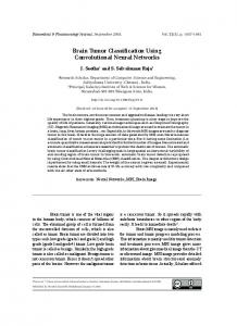
first utterance is the spoken word chain uttered by the caller in response to the operator greeting that explains his or her problem. This utterance was transcribed unless it was a greeting or phrase such as “yes er I’m wondering if you could help me” or “is that the operator? ”. In this case the second utterance of the caller was also transcribed. Therefore, in the case of example three in Table 1, the second utterance of the caller would also be transcribed beginning at “I wonder if er you can tell me ....”. The transcription of each recorded utterance has four attributes: a call, a call class, a primary move, and a request type as indicated by the example in Table 2. The call contains the utterance of the caller made in response to the operator greeting. The call class is related to the service that the caller request is routed to. The number of call classes in the task is 17 and a breakdown of the spread of each call class within each call set is provided in Figure 1 (Durston et al 2001). The segment of the utterance that signifies the primary move was enclosed in boundary markers ‘@@’ and assigned a primary move type. The primary move type is associated with the identified intention of the caller. The boundary markers ‘@@’ are not presented to the classifier. The markers are used during pre-processing to “tag” the

Call set 1

350

Call set 2

Call set 3

Call set 4

300 250 200 150 100 50 0 ln

rc

ac

ac−n

dq

dq−a

idq

idq−aCall ioa classes flt

cs

cs−n

bill

examples of call classes are: line test, alarm call, international operator, billing

Fig. 1. Number of each call class within each call set.

o−ref

o−op

tm

oth


5

Table 3. Example tagged call. yeah @@ (CALL could I book a wake up call please )CALL (CLASS @@, ac )CLASS (MOVE action )MOVE (TYPE exp )TYPE )END

transcription with the labels ‘(CALL’, ‘)CALL’, and ‘(CLASS’. As the task is classifying a caller utterance to a call class the primary move type is not used in the experimental work reported here. Further analysis of the corpus revealed that not all call classes are associated with each primary move type. As a result it is unlikely that certain service requests would be classified to a particular call class. Consequently if we were to classify based initially on the primary move type this could reduce the number of call classes available for selection. This could perhaps provide some good indicators for the future about either the types of dialogue or speech acts used by the callers or the vocabulary contained within the utterances to aid the classification process. The call class and the primary move type differ in their focus. The call class is more concrete and is associated directly with the service the caller requires. The primary move is more abstract and reflects what the caller is trying to achieve or what the intention of the caller is believed to be. “can you er get me British Telecom please on the erm payments” In the example above the call class is “bill ” because the caller requires referral to the billing service and the “primary move” is “connect” because the caller has indicated a requirement for a connection to another service. The request type identifies the style of language used by the caller to talk to the operator. Is the request for service expressed in explicit terms or is it an implicit request expressed by the use of free language (Durston et al 2001). The above utterance is an example of the latter. Before the classification task can be undertaken the transcribed utterances undergo some pre-processing. The individual segments of each utterance are manually “tagged”, as shown in the example tagged utterance, Table 3; call class becomes CLASS, primary move becomes MOVE and request type becomes TYPE. These labels are used as boundary markers for generating both the lexicon and the training and test sequences. The tagged utterances in each call set are processed and a lexicon in the form of a vector representation, that includes the frequency of occurrence of each word in a particular call class, is generated, as illustrated in Table 4. The labels are used to identify which words are added to the lexicon, that is only those words that occur between the (CALL and )CALL labels. The lables are also used to identify which call class the words are associated with between the (CLASS and )CLASS labels. All text outside of these labels is ignored. The labels appended to each utterance are not used in the input to the classifiers. The labels are only used in the processing of

6


Table 4. Example of semantic vectors. Note: For illustration purposes not all call classes are shown. There are 17 classes used in this study. Word

Call Class ln

rc

ac

ac-non

dq

dq-area

idq

class n

CAN YOU JUST CHECK TO SEE IF ITS OUT OF ORDER

0.03 0.07 0.18 0.53 0.08 0.36 0.12 0.19 0.10 0.09 0.24

0.06 0.01 0.00 0.00 0.06 0.00 0.08 0.00 0.00 0.00 0.00

0.09 0.01 0.00 0.00 0.01 0.00 0.02 0.00 0.00 0.00 0.54

0.07 0.05 0.00 0.00 0.05 0.00 0.00 0.06 0.00 0.11 0.00

0.05 0.09 0.03 0.00 0.02 0.00 0.06 0.04 0.02 0.14 0.00

0.08 0.10 0.03 0.00 0.01 0.00 0.10 0.06 0.12 0.01 0.00

0.04 0.05 0.00 0.11 0.05 0.00 0.05 0.01 0.00 0.03 0.00

... ... ... ... ... ... ... ... ... ... ...

the call set for the purpose of generating the lexicon and the training and test vector representations that are used to create the inputs for each of the classifier components.

2.4. Calls and Semantic Vectors In our experiments we use a semantic vector representation of the words in a lexicon (Wermter et al 1999). These vectors represent the frequency of a particular word occurring in a call class and are independent of the number of examples observed in each call class. The number of calls in a call class can vary substantially. Therefore we normalize the frequency of a word w in call class ci according to the number of calls in ci (2). A value v(w, ci ) is computed for each element of the semantic vector as the normalized frequency of occurrences of word w in semantic call class ci , divided by the normalized frequency of occurrences of word w in all call classes. That is: N ormalized f requency of w in ci =

F requency of w in ci N umber of calls in ci

(1)

where: N ormalized f requency of w in ci , i, j ∈ {1, · · · n} v(w, ci ) = P N ormalized f requency f or w in cj

(2)

j

Each call class is represented in the semantic vector. An illustrative example is given in Table 4. As can be seen in the illustrative example, domain-independent words like ‘can’ and ‘to’ have fairly even distributions which is to be expected as these are function words, while domain-dependent words like ‘check’ and ‘order’ have more specific preferences.

2.5. Training and Test Call Sets Four separate call sets each containing 1,000 utterances were used in this study. The four call sets were used individually as a baseline to establish how each of the classifiers performed with a view to scaling-up the investigation using the call sets in a crossvalidated approach and selecting the best classifiers. Testing each classifier on only one call set may not have provided a true indication of performance whereas testing on four call sets allows for variation in the call sets.


7

No. in Training Set

800

No. in Test Set No. Not Used

700 600 500 400 300 200 100 0 Call set 1

Call set 2

Call set 3

Call set 4

Fig. 2. Number of training and test examples per call set.

Table 5. Breakdown of utterances in training and test sets from call set 1. Note: For illustration purposes not all call classes are shown. 917 utterances Total of 712 utterances in Training set Total of 205 utterances in Test set Categories:

ln

rc

ac

ac-non

dq

dq-area

idq

class n

in train set: in test set:

261 59

11 3

41 21

3 1

85 29

32 11

6 2

... ...

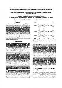
The call sets are split so that 80% of utterances are used for training and 20% of utterances used for testing. Only the part of the utterance identified as indicating the primary move was used for training and testing. As part of the pre-processing stage this part of the utterance was assigned a classification using the call class associated with the full transcription of the utterance. At this stage some utterances were excluded from the training and test sets because they did not contain a primary move utterance, which effectively means that utterances that contained phrases like “oh sorry wrong number ” were grouped into an other call class. A breakdown of the number of training and test examples per call set is provided in Figure 2. The average length of an utterance in the training set is 16.05 words and in the test set the average length of an utterance is 15.52 words. An illustrative example is given in Table 5 however not all call classes are shown. Entropy is associated with uncertainty or information in relation to the task of selecting one or more items from a set of items. Thus entropy is a measure of how many bits of information we are trying to extract in a task and it gives an indication of how certain or uncertain we are about the outcome of the selection (Charniak 1993). In addition, the concept of entropy provides an indication of problem difficulty and both high and low entropy values can indicate difficult problems. A low entropy value indicates diversity; an uneven class distribution with the classifiers being unable to learn the small classses well. A high value indicates more similarity and therefore greater difficulty in differentiating between items. To normalize the entropy value of a class to

8


Table 6. Example SRN input. (SEQ 32 IM TRYING TO GET A LONDON NUMBER )

I’m trying to get a London number 10000000000000000 10000000000000000 10000000000000000 10000000000000000 10000000000000000 10000000000000000 10000000000000000 category output representation

{z

|

}

0.16 0.34 0.08 0.22 0.14 0.46 0.15

0.00 0.00 0.04 0.00 0.11 0.00 0.01

0.00 0.01 0.01 0.02 0.06 0.00 0.00

0.00 0.00 0.03 0.00 0.03 0.00 0.00

... ... ... ... ... ... ...

word input representation

|

{z

}

Table 7. Example SVM input. +1

I’m 1:0.16

trying 2:0.34

to 3:0.08

get 4:0.22

a 5:0.14

London 6:0.46

number 7:0.15

the range [0, 1], the base of the logarithm is the number of utterances. In this task the four call sets under investigation each have an entropy of 0.31. entropy = −

17 X

P (ci )logn (P (ci )), where n is the number of utterances

(3)

i=1

2.6. Input Representations of Each Technique The focus of this work is the classification of a caller’s first utterance to one of a predefined number of call classes. To make any comparison as fair as is possible the same corpus and basic underlying representation was used as the basis for the input representations for each of the techniques. This means that the initial lexicon values generated from processing the corpus were converted into a feature representation format applicable to each technique. Although the techniques use different feature representations no changes were made to the lexicon values; therefore each representation was derived from the same basic representation. Consequently each technique is starting with the same underlying information from the corpus. An example of the respective representations used by each technique, for the same example, is provided in Tables 6, 7, and 8. For the SRN each utterance in the training or test set was allocated a sequence number, a category output representation, and a word input representation, as illustrated in Table 6. The category output representation represents the call class associated with the utterance and the word input representation represents the frequency of occurrence of each word. For the SVM the inputs are composed of feature-value pairs separated by a colon as shown in Table 7. For example, 1:0.16, the ‘feature,’ in this case ‘1’, is the position of the word in the utterance and the ‘value’, ‘0.16’, is the frequency of occurrence of that word in any position for the particular call class under investigation. An FST is constructed using regular expressions. To create the regular expressions each utterance in the call set is symbolically tagged. These symbolic tags enable identification of possible patterns or strings and substrings in the utterance. This means that each word in the utterance is tagged with a symbolic representation of the call class associated with that word based on the highest frequency of occurrence as shown in Table 8.


9

Table 8. Example FST input. I’m ln

trying ln

to ioa

get ln

a ln

London ln

number ln

Lexicon

Call File

Pre processing

+

Tagged Call Set

Input

Tagged Call Set Classification Component

Output

Fig. 3. Architecture of the system.

Thus in the lexicon, the word ‘I’m’ is most frequently associated with the ‘ln’ call class based on the frequency of occurrence. These symbolic tags represent the sequence for a specific utterance. This clearly shows the higher frequency of the ‘ln’ call class would indicate that this utterance is classified as an example of the ‘ln’ call class. There is no removal of function words such as ‘a’, ‘the’, and ‘and’ etc, since it has been indicated that they may serve important roles.

3. Architecture Figure 3 shows the general structure of our architecture, which combines different components. The pre-processing and generation of the lexicon were described in Section 2.3 and the call sets were described in Section 2.5. The lexicon together with the tagged call set are then used to generate the input, that is, the training and test sequences for the classification component of our architecture. The aim of the experimentation was to identify effective techniques for use in the classification component of our architecture.

3.1. Experiments Using Neural Networks, Support Vector Machines and Transducers We have considered using language models for this task but then focused on identifying alternative techniques that may have potential for use in the task of classifying a caller

10

S. Garfield and S. Wermter Call class A B C Total

Retrieved and Relevant (1) 55 19 1 75

Retrieved not Relevant (2) 7 2 1 10

Relevant not Retrieved (3) 4 10 4 18

utterance to a call class. A drawback to language models is that they require large amounts of transcribed and labelled training data from which to calculate the probabilities of the most likely word sequences. Additionally, language models are unable to model long distance dependencies (Stolcke et al 1998) because they are usually restricted to local regularities like bi-grams and tri-grams (Brill et al 1998; McTear 2002). In comparison, our approach adopted uses the continuous word sequence of the caller’s utterance from the corpus as supplied by the telecommunications collaborator rather than keywords or phrases. Our approach uses a shallow surface rather than a deep interpretation to produce a classification result, since this may be all that is required if the next stage were to be the handling of the call by an operator. The caller request is routed to a service and the operator extracts the details of the caller’s problem or enquiry. Details of the techniques used are provided in the subsequent sections. The performance of each technique will be evaluated using the evaluation metrics recall and precision (Salton and McGill 1983) and the F-score (Van Rijsbergen 1979). Recall and precision (Salton and McGill 1983) are standard measures of information retrieval performance. Recall and precision can be calculated using the following equations: Recall =

N umber of relevant utterances retrieved T otal N umber of relevant utterances in collection

P recision =

N umber of relevant utterances retrieved T otal N umber of utterances retrieved

The F-score (Van Rijsbergen 1979) is a combination of precision and recall and is a method for calculating a value without bias, in other words, without favouring either recall or precision and is calculated using the recall and precision values: F =

2 ∗ (R ∗ P ) (R + P )

For each call set, at the end of both the training and the testing phases three values were obtained for each call class for the following categories: (1) the number of utterances retrieved that were relevant, (2) the number of utterances retrieved that were not relevant, and (3) the number of relevant utterances not retrieved. For a call set the values for each call class were added together to produce a total value for each of the three categories. These totals were used to calculate the results for recall and precision that are used to calculate the F-score. A small illustrative example calculation for recall is provided below. Recall =

(1) (1) + (3)

75 75 + 18

= 80.65%

The section continues with a discussion of neural networks.

3.2. Neural Networks Several neural network architectures were used for the experiments ranging from a feedforward network with only one input and one output layer to a simple recurrent


11

network with input, output, hidden, and context layers. The feedforward network uses a system of error correction to adjust the network while it produces the required output. The actual output result is compared with the desired result and the weights are either strengthened or weakened by an amount proportional to the size of the error. This involves examining the sum of all the differences between the desired outputs and the actual outputs and reducing this error by a process of gradient descent (LeCun et al 1998). A recurrent neural network extends a feedforward network by introducing previous states and short-term incremental memory and can be either fully or partially recurrent. A partially recurrent network, such as a simple recurrent network, has recurrent connections between the hidden and context layers (Elman 1990) whilst a Jordan network has connections between the output and context layers (Jordan 1986). A key aspect of this network is that it allows the processing of sequences in a robust manner.

3.2.1. Training Environment Supervised learning techniques were used for training (Elman et al 1996; Wermter 1995) which requires presentation of both the required output and the input stimulus. The weights of an untrained network are initialised to small random numbers. In one epoch, or cycle, of training through all training samples the network is presented with all utterances from the training set and the weights are adjusted at the end of each utterance. The training algorithm used compares the actual output to the desired output and calculates the difference so that the output produced comes a little closer to the desired output (LeCun et al 1998). The input layer has one input unit for each call class. During training and testing, utterances are presented sequentially to the network one word at a time. Each input unit receives the value of v(w, ci ), where ci denotes the particular call class of a word w which the input is associated with. Utterances are presented to the network as a sequence of word input and category output representations, one pair for each word. At the beginning of each new utterance the context layers are cleared and initialised with 0 values. Each unit in the output layer corresponds to a particular call class and the output unit that represents the desired call class is set to 1 and all other output units are set to 0. Although several neural network architectures were used only the performance of the simple recurrent network (SRN) is reported since this architecture was more successful than either the feedforward or the Multi-Layer-Perceptron (MLP) due to its additional memory. The results produced by the feedforward network suggested that this network did not have sufficient processing capacity. Likewise, even the MLP with one hidden layer did not have sufficient context processing capacity to handle the sequential inputs.

3.2.2. Simple Recurrent Neural Network The SRN (Elman et al 1996; Wermter 2000; Wermter 1995), depicted in Figure 4, uses a set of context units which copy their activations (values) from the hidden units. The hidden units also receive input from the context units. The hidden units are updated first before the context units copy the hidden units’ values and provide input to the hidden units. Therefore the context layer enables the output values of the network’s hidden units to be stored and then re-used in the network by providing the hidden layer with the pattern of the previous activation state (Wermter et al 1999; Elman 1991). While Figure 4 shows the most basic SRN other, more complex, recurrent networks have been examined in (Wermter 1995). An SRN with input, output, hidden, and context layers was used for our experiments. Training was carried out using supervised learning techniques (Elman et al 1996; Wermter 1995). In general, the input to a hidden layer Ln is constrained by the underlying layer Ln−1 as well as the incremental context layer Cn . The activation of a unit Lni (t) at time t is computed on the basis of the

12


L2

output units

L1 hidden units copy context units

L0

Cn

input units

Fig. 4. Simple recurrent network.

weighted activation of the units in the previous layer L(n−1)i (t) and the units in the current context of this layer Cni (t) limited by the logistic function f .

X

Lni (t) = f (

k

wki L(n−1)k (t) +

X

wli Cnl (t))

(4)

l

This provides a simple form of recurrence that can be used to train networks to perform sequential tasks over time which means the output of the network not only depends on the input but also on the state of the network at the previous time step. Events from the past can be retained and used in current computations, that is, the output at time t is re-used as the input at time t + 1. This allows the network to produce complex time-varying outputs in response to simple static input which is important when generating complex behaviour. As a result the addition of recurrent connections can improve the performance of a network and provide the facility for temporal processing (Wermter et al 1999). While the architecture of the neural network component was adjusted in relation to the number of layers in the network the strategy for training, that is to say, the learning rate (0.01, 0.006 and 0.001), momentum term (0.8), and number of epochs of training (1,000) remained constant. The initial learning rate of 0.01 changed at 600 epochs to 0.006 and again at 800 epochs to 0.001. The network was trained on the four call sets using this training strategy. The addition of a second hidden layer, a context layer, which was used to add sequential memory to the network produced a significant improvement in network performance, see Figure 5. The recall rate after testing on the test set for call set one increased to 79%. This was a difference in improvement of over 51% on the previous best recall rate achieved by the feedforward network. The difference in improvement in performance on the test set for call set one was over 45% when compared to that of the MLP network. Overall, when tested, the difference in improvement in recall rate achieved by the SRN ranged from 49.5% to 57.9% when compared to the recall rate for the MLP network trained using the same strategy of 1,000 epochs and a changing learning rate. Then the SRN was trained again on the four call sets using a different learning strategy. In this strategy the learning rate was fixed at 0.01, the number of epochs of training remained constant at 1,000, and the momentum term also remained unchanged at 0.8. The recall rate of 76.6% on the test set for call set one is slightly lower, by 2.4%, than the recall rate of the network trained with a changing learning rate whilst the precision rate is only lower by 0.8%. The performance of the network varied slightly across the call sets and the use of a fixed learning rate did produce some improvement in performance but only


13

100.00% 90.00% 80.00% 70.00% 60.00%

Call set 1

50.00%

Call set 2 Call set 3 Call set 4

40.00% 30.00% 20.00% 10.00% 0.00% Recall

Precision

Fig. 5. Test results of simple recurrent network (SRN). Table 9. F-Score results for the simple recurrent network.

Call Call Call Call

set set set set

1: 2: 3: 4:

Training Set

Test Set

F-Score

F-Score

89.49 88.31 90.27 89.14

84.37 80.93 80.42 80.63

on two of the call sets compared to the network trained with a changing learning rate. Overall there was a significant increase in performance when compared to the feedforward and the MLP networks trained with the same fixed learning rate. The F-score (Van Rijsbergen 1979) performance of the trained SRN on the four call sets, which is a combination of the precision and recall rates, is shown in Table 9. The recall and precision performance is shown in Figure 5. There is a difference of 3.5% and 5.1% between the highest and the lowest test recall and precision rates respectively. In conclusion, simple recurrent networks performed substantially better than simple perceptrons or feedforward networks.

3.3. Support Vector Machines Since support vector machines have been shown to be good statistical classifiers we wanted to compare our results with them. Neural networks use the Empirical Risk Minimisation (ERM) principle which minimises the error on the training data while the Support Vector Machine (SVM) developed by Vapnik (Vapnik 1995) uses the Structural Risk Minimisation (SRM) principle which minimises an upper bound on the generalisation error (Gunn 1998; Burges 1998; Joachims 2000; Scholkopf 1998). An SVM is a binary classifier and the SVM approach divides the problem space into two regions

14


support vectors margin

h (hyperplane)

Fig. 6. Optimal separating hyperplane.

via a dividing line or hyperplane with a classifier referred to as the optimal separating hyperplane, Figure 6. This hyperplane separates positive examples from negative examples with a maximum margin (Chapelle and Vapnik 2000; Opper and Urbanczik 2001; Platt 1998; Feng and Williams 2001) between it and the nearest data point of each class. SVMs can deal with non-linearly separable cases, ie, where a straight line cannot be found, and can handle noisy data (Platt 1998). SVMs make use of kernels (Moghaddam and Yang 2001; Opper and Urbanczik 2001) therefore all computations are performed directly in input space and depending on the kernel function used, for example, polynomial, radial basis function (RBF), and sigmoid, different types of classifier can be constructed (Stitson et al 1996; Moghaddam and Yang 2001; Scholkopf et al 1995). One potentially problematic area is the optimisation of the kernel parameters and choosing the right combination of parameters.

3.3.1. Support Vector Machine Experiments In order to compare the performance of the SRN to other classification approaches a series of experiments was conducted using an SVM with different kernel functions: polynomial, RBF, and sigmoid. The value for the tuning or trade-off parameter C, the error penalty (Joachims 1999; Joachims 2002), was chosen based on empirical experience. This parameter allows a trade-off between the margin width and classification error (Joachims 1999; Joachims 2002). Several values for C were investigated in order to determine a value that reduced the test error to a minimum while at the same time constructing a classifier that was able to perform successfully on the individual categories. The value for C used in the experiments was 64. Other parameters that could be set for each kernel and were the same across the kernels were kept constant which means the classifiers were constructed using the same values. A classifier was constructed (Joachims 1999) for each call class and the training and test sets were generated from the same utterance sequences from the same four call sets. The training approach adopted was one-versus-all, that is to say, the training and test sequences used positive examples for the particular call class in question and negative examples of all the other call classes. The classifier in each case was trained and then tested on these sequences. On completion of the training phase a model is generated which is then used in the testing phase. In their basic form the decision function that determines whether a


15

Table 10. F-Score results of SVM. Training Set

Call Call Call Call

set set set set

1: 2: 3: 4:

Test Set

RBF

Sigmoid

Polynomial

RBF

Sigmoid

Polynomial

89.31 89.89 88.92 91.23

75.70 81.06 79.78 84.09

77.00 81.77 78.50 83.92

56.71 58.46 57.88 57.57

57.82 60.51 59.58 60.51

64.36 63.82 66.66 65.26

90.00%

Call set 1 Call set 2 Call set 3

80.00%

Call set 4

70.00%

60.00%

50.00%

40.00% Recall

Precision

RBF

Recall

Precision

Sigmoid

Recall

Precision

Polynomial

Fig. 7. Test results of support vector machine (SVM).

test example is classified can be described by a linear hyperplane h, attribute vector x, weight vector w, and a threshold b, and takes the form of: h(x) = sign(w ∗ x + b)

(5)

where the output is: +1 if w * x + b > 0, and -1 otherwise. The F-score performance for each of the trained classifiers on the four call sets is shown in Table 10. The test recall and precision rates for each of the different classifiers is shown in Figure 7. These results are for the individual classifiers trained and tested using constant parameter values. The classifier constructed with the RBF kernel achieved the best test performance figures for recall on each of the four call sets when compared to both the sigmoid and polynomial kernels. The classifier constructed with a polynomial kernel achieved greater test performance figures for precision on all four call sets than the other two kernels. Across the four call sets there is a difference of some 5% between the highest and

16


a:[]

1 a:d b:[] b:d 0

2

b:[] c:[]

c:d

c:[]

3

Fig. 8. A transducer encoding a relation denoted by a regular expression.

lowest test recall and test precision rates for the RBF kernel classifier. For the sigmoid kernel classifier the difference is some 6% for test recall and some 3% for test precision. Therefore, for both of these kernel types the difference is smaller for test precision. In the case of the polynomial kernel classifier, the difference between the highest and the lowest rates is smaller for test recall than test precision; this is opposite to the results for the RBF and sigmoid kernel classifiers.

3.4. Finite-State Automata and Transducers Finite-state automata and transducers or finite-state machines could prove useful in this task for several reasons. Firstly, finite-state machines are well understood and clearly defined and can be small in size. Secondly, their representation and their output is easy both to understand and interpret: their representation is symbolic in nature and they use as their basic unit a string. Therefore, it is relatively easy to input data. Finally, finite-state machines can handle strings of any length. This is of particular significance in this task because the length of the caller’s utterance is variable. A finite-state machine is a formal machine that consists of states, arcs that represent transitions, one start state, any number of final states, and an alphabet (Roche and Schabes 1997; Jurafsky and Martin 2000). A finite-state machine operates on strings. A string is a sequence of symbols composed from an alphabet and an alphabet is a set of symbols or characters. Computation in a finite-state machine begins at the start state with an input string and the transitions change from one state to other states. Finite-state machines can either be simple automata that encode regular languages or transducers that represent a regular relation which is a set of pairs of strings, as illustrated in Figure 8. A transducer maps between one set of symbols and another and can recognise or generate pairs of strings. As a result one view of a transducer is a machine that reads one string and generates another. For example the transducer in Figure 8 encodes the relation denoted by the regular expression (a∗ b∗ c) → d

(6)

that is, the transducer would recognise sequences such as (aaabbbc) and generate a “d ” as output.


17

Table 11. F-Score test results of FST. Test Set Call Call Call Call

set set set set

1: 2: 3: 4:

40.03 40.56 44.73 37.90

3.4.1. Construction of Transducers from Regular Expressions Finite-state machines can be specified using regular expressions. A regular expression specifies how patterns or strings and substrings can be created. The strings and substrings are created by combining symbols, in other words, characters or words that have been extracted from a restricted alphabet or vocabulary. The order in which symbols in the strings and substrings can be joined together is indicated by the regular expression. The expression also indicates whether for each position there are other possible alternatives for symbols and whether or not it is possible to repeat these strings and substrings. In order to create the regular expressions the utterances in the call set are symbolically tagged to enable identification of possible patterns or strings and substrings in the utterances, as illustrated in Section 2.6.

3.4.2. Transducer Experiments To enable a comparison between transducers and the other classification techniques outlined, a series of experiments was conducted. The same four call sets of utterances were used as in previous experiments and transducers were constructed for each call class. Each utterance in the training sets was converted into a symbolic representation of the call class associated with each word based on the highest frequency of occurrence. Then transducers were constructed for each call class from regular expressions which were hand-crafted. The converted training sets were used as reference sets whilst creating the regular expressions based on sequences of call classes identified in the symbolic representation of the utterances. Once the transducers were constructed each was tested against the test sets for the other call classes. The transducer produces an output class for each sequence. A successful output is the semantic label of the call class for which the transducer has been constructed while an unsuccessful output is ‘0’. For the call class for which the transducer was constructed the number of successful outputs generated were counted as utterances that were retrieved and relevant and the number of unsuccessful outputs were counted as relevant utterances not retrieved. Successful outputs on call classes that were not the call class for which the transducer was constructed were counted as utterances retrieved that were not relevant. Using these values the recall, precision, and F-score results were calculated for each call set, see Section 3.1. The test F-score results for each of the four call sets are provided in Table 11. The test recall and precision results for each of the four call sets are shown in Figure 9. For some of the call classes the regular expressions were so prescriptive that the transducer achieved 100% performance on its own individual sequences and the error rate on the other sets was low. This performance is useful if the transducers are to be used as a means of exception handling or identifying those sequences that a recurrent neural network cannot classify. On the other hand for one or two call classes the regular expressions identified were more general because the transducers also generated output for the other call classes. Based on the performance of these transducers it has been demonstrated that it can be difficult to create a specific regular expression for some call classes because the semantic content of the utterances in some call classes does at times closely respesent that of other call classes, as in the examples shown below

18


70.00%

1

65.00% 2

60.00%

3

4

Call Set 1 Call Set 2 Call Set 3 Call Set 4

55.00% 50.00% 45.00% 40.00%

3

35.00% 1

30.00%

2

4

25.00% 20.00% 15.00% 10.00% 5.00% 0.00% Recall

Precision

Fig. 9. Test results of finite-state transducers (FST). Table 12. Example of overlapping classes. can can

you you

check check

a my

line line

for is

me working

please properly

ln flt

in Table 12, and therefore it is problematic to correctly identify the appropriate call class. Given this, for these call classes the recurrent neural network has proven more successful as it is better able to handle more difficult semantic sequences due to its generalisation ability.

3.5. Classifier Processing Time The processing time for the SRN and the SVM with respect to training varies; FSTs do not require training but creating regular expressions is a time-consuming process. The time taken to create the regular expressions varied depending on the call class and the number of examples in the training sets. This is because the training sets, which were used as reference sets, had to be examined manually to identify sequences of call classes and the sequences were used to create the regular expressions. This process may take less than one hour or several hours for a human depending on the call class. The shortest computer training time for the SRN was 3 hours 30 minutes and the longest training time was 5 hours 30 minutes. The training time for the SVM not only varied depending on the call class but also the kernel being used and the kernel parameter values selected. The SVM training time was considerably faster than the SRN, at under one minute, although performance of the SRN was much better. The SVM training used a one-versus-all method, see Section 3.3.1, that is each SVM was trained on one call class against all the other call classes whereas the SRN was trained on 17 call classes at the same time. Optimisation of the SVM is an integral and automatic part of the training process. The SVM software (Joachims 1999) employs a fast optimisation


19

algorithm where the number of members of the working set of examples are selected according to a steepest feasible descent strategy.

4. Analysis and Discussion To establish what effect factors such as number of network layers and learning rate have on network performance these elements were changed and several experiments conducted to determine the effects of these changes. Overall changes to the learning rate had little effect on the performance of the feedforward network. The results show that with or without a constant learning rate the network was only able to correctly classify on average 21.91% of the utterances. There was however a slight negative effect on performance of the MLP network by changes to the learning rate. The network trained using a constant learning rate of 0.01 was able to correctly classify on average 23.83% of all utterances whilst with changes to the learning rate the network was only able to correctly classify on average 22.53% of all utterances, a drop in performance of 1.3%. On average the SRN was able to correctly classify over 75% of all utterances with or without changes to the learning rate. Therefore changes to the learning rate on the SRN had only a slight effect on performance. This suggests that the biggest factor in improving the network performance was the addition of the context layer. Analysis of the performance of the SVM on the classification of some of the utterances identified several factors, one of which is the trade-off parameter C. If the parameter value is low the SVM produces a simple decision surface and subsequently lots of misclassification errors, while a high value produces a complex decision surface and good classification. Another key factor is the type of kernel function used and how much the individual parameters are tuned. As with the trade-off parameter C, altering other parameters also has an effect on the recall and precision performance of the SVM. Changes, for example, to the value of the reciprocal of the Gaussian function in the RBF kernel in conjunction with the trade-off parameter C cause the classifier to improve performance in one area, in this case, recall yet decrease it in the other, in this case, precision. The aim therefore is to find a balance that provides an acceptable level of recall with an acceptable level of precision. In these experiments the parameter values were kept constant for each kernel type. However, it is likely that using parameter values tuned specifically for each kernel will produce better results on some call classes than others. The FST, unlike the other two classifiers, relies on regular expressions that are hand-crafted. This process, as described in Section 3.4.1, is both time consuming and labour intensive. In most instances the transducer is able to correctly classify utterances to the appropriate call class and reject those utterances that do not belong to the call class under investigation. Overall, the FST was able to classify examples belonging to all call classes but the performance was lower than that of the SRN. This means that the FST was able to produce a classification result for utterances associated with each call class, while the SRN and SVM in some cases were unable to produce a classification result for utterances associated with six of the call classes in total across all four test sets. For the SVM the inability to classify some of the call classes could be related to the type of kernel function chosen. All kernel types: RBF, sigmoid, and polynomial had problems with two or more call classes. One reason why classifiers such as the SRN and SVM are unable to classify utterances associated with certain call classes could be that these particular call classes have few examples in both the training and test sets in comparison to other call classes; both of these techniques learn from examples while the FST relies on hand-crafted regular expressions. One call class that both the SVM and the SRN were able to classify constitutes 36.66% of the training set and 28.78% of the test set and one call class that both techniques had problems classifying constitutes only 0.42% of the training set and only 0.49% of the test set. However, only a small increase in the overall representation

20


Table 13. Test Set - Comparison of F-score results for simple recurrent network (SRN), support vector machine (SVM), and finite-state transducer (FST). F-score

SRN SVM: RBF Sigmoid Polynomial FST

Call set 1

Call set 2

Call set 3

Call set 4

84.37

80.93

80.42

80.63

56.71 57.82 64.36 40.03

58.46 60.51 63.82 40.56

57.82 59.58 66.66 44.73

57.57 60.51 65.26 37.90

of a call class can be sufficient to enable both techniques to classify that call class, eg, 1.54% of the training set and 1.46% of the test set. The improvement in the classifiers’ ability to classify utterances resulting from a small increase in the number of examples raises the issue of whether to manipulate the number of examples to produce a more balanced distribution. This issue was not considered for this work because we wanted to establish how well the classifiers could handle the task using the corpus as supplied by our telecommunications collaborator where the distribution of examples is representative of the call traffic to the operator assistance service. Other possible reasons could be related to the vocabulary used in the utterances associated with these problematic call classes or the length of the utterances. Neural networks are inclined to learn first those classes that occur more frequently, that is, those classes they “see” more of before learning those that are less frequent. SVMs rely on labelled training data as well as patterns in the data to characterise the classification function that maximises the margin between the classes and at the same time minimises the number of support vectors. If there are few samples of the class to be learned it is likely therefore that it will be difficult for the classifier to identify the patterns or support vectors needed. The evaluation metrics chosen to measure performance of the classifiers were selected because the task was approached as a classification task and recall and precision are standard measures of classification performance. When comparing classifiers using only one evaluation measure may be preferable because using only one measure makes comparison simpler. Consequently the F-score is used as the comparison metric. The F-score performance of the SRN, SVM, and the FST on the test sets for the four call sets is summarised in Table 13. From the results on the test sets, shown in Table 13, it is evident the performance varies across each technique. Generally, the performance of the SRN is better than that of the SVM and the FST. While the results of the SRN would seem to indicate that the use of transcripts of the spoken word chain were beneficial to performance this would not seem to be true based on the results of the SVM and the FST. Their performance overall is considerably lower than that of the SRN and therefore for these classifiers does not seem to provide additional benefit. This is a possible indication that the method of representation of the semantic content of the utterances for the SVM and the FST is not optimal and does not allow either technique to consistently classify the utterances. Based on the very low performance of the FST it is evident that the hand-crafted regular expressions do not capture a fine enough level of granularity in the semantics of the utterance for the FST to accurately classify the utterances. Another factor to consider is the number of examples in each of the call classes. The number of examples in the ‘ln’ call class is over five times greater than that of the ‘ac’ call class. As a result, if one or two examples are misclassified or not classified in a small number of examples the impact on the result, in percentage terms is much greater and produces a greater difference to the result but the same is not true for a larger set of examples. In general, the F-score results for the SRN are quite high given


21

the number of call classes available against which each utterance can be classified. The SRN achieved an average F-score performance of 81.59. This result is calculated based on the performance figures for the SRN shown in Figure 5. In other related work on call routing the evaluation measures used are false rejection rate: a call is rejected or classified as ‘other’ and the call is routed to the operator when it could have been automatically routed, and probability of correct classification, that is how often the classifier is correct. On transcribed calls Gorin et al (1997) achieved a probability of correct classification rate of 84% with a false rejection rate of 10%, while in the OASIS project the accuracy rate of the classifier was approximately 75% on transcribed data (Chou et al 2000). The vector-based approach of Chu-Carroll and Carpenter (1998) achieved an overall classification performance in the range of 77%97% and on transcribed calls a classification performance of approximately 94% with a rejection rate of 10%. A key factor in the approach of Chu-Carroll and Carpenter is the use of a disambiguation module; Chu-Carroll and Carpenter acknowledge that the disambiguation module does govern performance. While these comparisons give some illustration of the difficulty of classifying spontaneous language, the corpus and evaluation metrics used differ. The focus of the evaluation measures used by those working on the task of call routing appears to be the ability of the classifier to either reject a call or label the call as ‘other’ whereas the focus of our approach is how successfully the classifier can classify all call classes. Our classification task used an unbalanced real data set and using accuracy as the evaluation metric may have produced false or confusing results (Forman 2002) because accuracy results can be affected if one class is scarce; in this case recall and precision may provide a better alternative. The F-score can be used to evaluate performance on unbalanced data sets because this gives the harmonic mean of recall and precision and is often a preferable measure for this type of data set (Forman 2002). The F-score results reported show the potential of these techniques and the focus is a comparison of the performance among these techniques on the task of call classification and is not intended as a direct comparison with the work of Gorin et al or Chu-Carroll and Carpenter. It is acknowledged that there are other methods available for comparing performance. For future work the methods of other researchers investigating spoken dialogues could be investigated (Yang et al 2002; Gorin et al 2000).

5. Conclusions The performance of SRNs, SVMs, and FSTs has been discussed and a comparison made to the work of other researchers in the field of call routing. The main result from this work is that the performance of the SRN was best, in particular when factors such as irregularities in the utterance and the number of call classes are taken into consideration. However, a combination of techniques might yield even better performance. The SVM allows a trade-off between recall and precision and as a result for call classes that are problematic to the SRN the SVM might be a better alternative. Whilst the FST does not allow a trade-off between recall and precision again it could be used for those call classes that are problematic because it can achieve almost perfect performance, that is 100%, on both recall and precision. The drawback to this approach is that it requires hand-crafted regular expressions which are time-consuming to construct. One additional factor that must be considered is the number of examples available for training and testing as this does influence performance. This work makes a novel contribution to the field of classification using a large, unique corpus of spontaneous spoken language. Based on transcribed, segmented utterances it has been demonstrated that an SRN performed best for spoken language classification. From the perspective of the other techniques identified it has been demonstrated that there is potential in SVMs and FSTs, for example for exception handling, for spoken language classification, but overall the SRN achieved a better performance

22


on this classification task, and therefore may be a useful main component for a hybrid architecture. Future work could focus on using alternative approaches such as Latent Semantic Analysis (LSA) to create a feature representation that provides a deeper meaning for the words in the utterances based on relationships identified between the words (Landauer et al 1998). This means that performance is not dependent on the choice of words and classification may still be achieved even if utterances have no words in common because LSA considers semantic similarity. Additionally, stochastic finite-state transducers, which can be learned efficiently from data using pairs of source and target utterances, could be adopted as they have been used successfully in research on the call routing task (Arai et al 1999).

References Allen J, Ferguson G, Ringger EK et al (2001) Dialogue Systems: From Theory to Practice in TRAINS-96. In: Dale R, Moisl H, Somers H (eds). Handbook of Natural Language Processing, Marcel Dekker, New York, pp 347–376 Allen J, Ferguson G and Stent A (2001) An Architecture for More Realistic Conversational Systems. Proceedings of Intelligent User Interfaces (IUI-01), Santa Fe, NM Arai K, Wright JH, Riccardi G et al (1999) Grammar Fragment Acquisition using Syntactic and Semantic Clustering. Speech Communication 27:43–62 Attwater D, Edgington M, Durston P et al (2000) Practical issues in the application of speech technology to network and customer service applications. Speech Communication 31:279– 291 Brill E, Florian R, Henderson JC et al (1998) Beyond N-Grams: Can Linguistic Sophistication Improve Language Modeling?. In: Boitet C, Whitelock P (eds). Proceedings of the ThirtySixth Annual Meeting of the Association for Computational Linguistics and Seventeenth International Conference on Computational Linguistics, Morgan Kaufmann Publishers, San Francisco, California, pp 186–190 Burges CJ (1998) A Tutorial on Support Vector Machines for Pattern Recognition. Data Mining and Knowledge Discovery 2:121–167 Burton-Roberts N (1986) Analysing Sentences. An Introduction to English Syntax. Longman Group UK Ltd, England Carpenter B, Chu-Carroll J (1998) Natural Language Call Routing: A Robust Self-Organizing Approach. ICSLP 98, Sydney, pp 2059–2062 Chapelle O, Vapnik V (2000) Model Selection for Support Vector Machines. In: Solla S, Leen T, Muller K-R (eds). Advances in Neural Information Processing Systems 12, MIT Press, Cambridge MA Charniak E (1993) Statistical Language Learning. MIT Press, Cambridge MA, USA Chou W, Zhou Q, Kuo H-K J et al (2000) Natural Language Call Steering for Service Applications. Proceedings of the International Conference on Spoken Language Processing, Beijing, China Chu-Carroll J, Carpenter B (1998) Dialogue Management in Vector-Based Call Routing. COLING-ACL98, pp 256–262 Chu-Carroll J, Carpenter B (1999) Vector-Based Natural Language Call Routing. Journal of Computational Linguistics 25(3):361–388 Durston PJ, Farrell M, Attwater D et al (2001) OASIS Natural Language Call Steering Trial. Proceedings of Eurospeech Vol. 2, pp 1323–1326 Edgington M, Attwater D, Durston P (1999) OASIS - A Framework for Spoken Language Call Steering. Proceedings of Eurospeech ’99, Budapest Hungary, pp 923–926 Elman JL, Bates EA, Johnson MH et al(1996) Rethinking Innateness. MIT Press, Cambridge MA, USA Elman JL (1991) Distributed representations simple recurrent networks and grammatical structure. Machine Learning 7:195–225 Elman JL (1990) Finding Structure in Time. Cognitive Science 14:179–211 Feng J, Williams P (2001) The Generalization Error of the Symmetric and Scaled Support Vector Machines. IEEE Transactions on Neural Networks 12(5):1255–1260 Ferguson G, Allen JF (1998) TRIPS: An Integrated Intelligent Problem-Solving Assistant. Pro-


23

ceedings of the Fifteenth National Conference on Artificial Intelligence (AAAI-98), Maddison, WI, pp 567–573 Forman G (2002) Choose Your Words Carefully: An Empirical Study of Feature Selection Metrics for Text Classification. 13th European Conference on Machine Learning ECML ’02 and 6th European Conference on Principles and Practice of Knowledge Discovery in Databases PKDD, Helsinki, Finland Garner PN (1997) On topic identification and dialogue move recognition. Computer Speech and Language 11:275–306 Glass JR (1999) Challenges for spoken dialogue systems. Proceedings of IEEE ASRU Workshop, Keystone, CO Gorin AL, Riccardi G, Wright JH (1997) How may I Help you?. Speech Communication 23:113– 127 Gorin AL, Wright JH, Riccardi G et al (2000) Semantic Information Processing of Spoken Language. Proceedings of 2000 International ATR Workshop on Multilingual Speech Communication, Kyoto Japan, October 2000, pp 13–16 Gunn S (1998) Support Vector Machines for Classification and Regression. ISIS Technical Report Harman D (1995) Overview of the Fourth Text REtrieval Conference. Proceedings TREC Joachims T (1999) Making Large-Scale SVM Learning Practical. In: Sch¨ olkopf B, Burges C, Smola A (eds). Advances in Kernel Methods: Support Vector Learning, MIT Press, Cambridge MA Joachims T (2000) Estimating the Generalization Performance of an SVM Efficiently. Proceedings of International Conference on Machine Learning Joachims T (2002) Learning to Classify Text Using Support Vector Machines. Kluwer Academic Publishers, Boston Jordan M (1986) Attractor Dynamics and Parallelism in a Connectionist Sequential Machine. Proceedings of the Eighth Annual Conference of the Cognitive Science Society , Amherst, pp 531–546 Jurafsky D, Martin JH (2000) Speech and Language Processing. Prentice Hall, Upper Saddle River, New Jersey Landauer TK, Foltz PW, Laham D (1998) An Introduction to Latent Semantic Analysis. Discourse Processes 25: 259–284 LeCun Y, Bottou L, Orr G et al (1998) Efficient BackProp. In Orr G, Muller K (eds). Neural Networks: Tricks of the trade, Springer McDonough J, Ng K, Jeanrenaud P et al (1994) Approaches to topic identification on the switchboard corpus. Proceedings of IEEE International Conference on Acoustics Speech and Signal Processing, Adelaide Australia, pp 385–388 McTear MF (2000) Intelligent interface technology: From theory to reality?. Interacting with Computers 12:323–336 McTear MF (2002) Spoken Dialogue Technology: Enabling the Conversational User Interface. ACM Computing Surveys 34(1):90–169 Moghaddam B, Yang M-H (2001) Sex with Support Vector Machines. In: Leen TK, Dietterich TG, Tresp V (eds) Advances in Neural Information Processing Systems 13, MIT Press, Cambridge MA, pp 960–966 Opper M, Urbanczik R (2001) Universal learning curves of support vector machines. Physical Review Letters 86(19):4410–4413 Platt JC (1998) Sequential Minimal Optimization: A Fast Algorithm for Training Support Vector Machines. Technical Report MSR-TR-98-14 Pyka C (1992) Management of hypotheses in an integrated speech-language architecture. Proceedings of 10th European Conference on Artificial Intelligence Roche E, Schabes Y (1997) Finite-state language processing. MIT, London Salton G, McGill M (1983) Introduction to Modern Information Retrieval. McGraw Hill, New York Sch¨ olkopf B (1998) SVMs - A practical consequence of learning theory. IEEE Intelligent Systems pp 18–21 Sch¨ olkopf B, Burges C, Vapnik V (1995) Extracting Support Data for a Given Task. In: Fayyad UM, Uthurusamy R (eds). Proceedings First International Conference on Knowledge Discovery and Data Mining AAAI Press, Menlo Park CA, pp 252–257 Stitson MO, Weston JAE, Gammerman A et al (1996) Theory of Support Vector Machines. Technical Report CSD-TR-96-17 Stolcke A, Shriberg E, Bates R et al (1998) Dialog Act Modeling for Conversational Speech.

24


Proceedings of AAAI-98 Spring Symposium on Applying Machine Learning to Discourse Processing Van Rijsbergen CJ (1979) Information Retrieval. 2nd edition. Butterworths, London Vapnik VN (1995) The Nature of Statistical Learning Theory. Springer-Verlag, New York Inc Wermter S (1995) Hybrid Connectionist Natural Language Processing. Chapman and Hall Thomson International, London, UK Wermter S, Panchev C, Arevian G (1999) Hybrid Neural Plausibility Networks for News Agents. Proceedings of the National Conference on Artificial Intelligence, Orlando, USA Wermter S, Weber V (1997) SCREEN: Learning a Flat Syntactic and Semantic Spoken Language Analysis. Journal of Artificial Intelligence Research 6(1):35–85 Wermter S (2000) Neural Fuzzy Preference Integration using Neural Preference Moore Machines. International Journal of Neural Systems 10(4):287–309 Wermter S (1999) Preference Moore machines for nueral fuzzy integration. Proceedings of the International Joint Conference on Artificial Intelligence, Stockholm, pp 840–845 Wermter S, Panchev C, Houlsby J (1999) Language disorders in the brain: Distinguishing aphasia forms with recurrent networks. AAAI 99 Conference Workshop on Neuroscience and Neural Computation, Orlando, USA, pp 93–98 Yang Y-J, Chien L-F, Lee L-S (2002) Speaker Intention Modeling for Large Vocabulary Mandarin Spoken Dialogues. ICSLP ’96 Vol. 2, pp 713–716 Young SR, Hauptmann AG, Ward WH et al (1989) High level knowledge sources in usable speech recognition systems. Communications of ACM 32:183–194

Author Biographies Sheila Garfield received a BSc (Hons) in Computing from the University of Sunderland in 2000 where, as part of her programme of study, she completed a project associated with aphasic language processing. She received her PhD, from the same university in 2004, for a programme of work connected with hybrid intelligent systems and spoken language processing. In her PhD thesis she collaborated with British Telecom and suggested a novel hybrid system for call routing. Her research interests are natural language processing, hybrid systems, intelligent systems.

Stefan Wermter holds the Chair in Intelligent Systems and is leading the Intelligent Systems Division at the University of Sunderland, UK. His research interests are intelligent systems, neural networks, cognitive neuroscience, hybrid systems, language processing, and learning robots. He has a diploma from the University of Dortmund, Germany, an MSc from the University of Massachusetts, USA and a PhD and Habilitation from the University of Hamburg, Germany, all in Computer Science. He was a Research Scientist at Berkeley, USA before joining the University of Sunderland. Professor Wermter has written, edited, or contributed to 8 books and published about 80 articles on this research area.