10th International Electronic Conference on Synthetic Organic Chemistry (ECSOC-10). 1-30 November 2006. http://www.usc.es/congresos/ ecsoc/10/ECSOC10.htm & http://www.mdpi.org/ecsoc-10/ [c012]
Predicting Human Immunodeficiency Virus (HIV) Drug Resistance using Recurrent Neural Networks Isis Bonet1*, Maria M. García1, Sain Salazar1, Robersy Sanchez2, Yvan Saeys3, Yves Van de Peer3 and Ricardo Grau1 1
Center of Studies on Informatics, Central University of Las Villas, Santa Clara, Villa Clara, Cuba, 2 Research Institute of Tropical Roots, Tuber Crops and Banana (INIVIT), Biotechnology Group, Santo Domingo, Villa Clara, Cuba, 3 Department of Plant Systems Biology, Flanders Interuniversity Institute for Biotechnology (VIB), Ghent University, Belgium
Abstract Motivation: Predicting HIV resistance to drugs is one of many problems for which bioinformaticians have implemented and trained machine learning methods, such as neural networks. Predicting HIV resistance would be much easier if we could directly use the three-dimensional (3D) structure of the targeted protein sequences, but unfortunately we rarely have enough structural information available to train a neural network. Furthermore, prediction of the 3D structure of a protein is not straightforward. However, characteristics related to the 3D structure can be used to train a machine learning algorithm as an alternative to take into account the information of the protein folding in the 3D space. Here, starting from this philosophy, we select the amino acid energies as features to predict HIV drug resistance, using a specific topology of a neural network. Results: In this paper, we demonstrate that the amino acid energies are good features to represent the HIV genotype. In addition, it was shown that Bidirectional Recurrent Neural Networks can be used as an efficient classification method for this problem. The prediction performance that was obtained was greater than or at least comparable to results obtained previously. The accuracies vary between 81.3% and 94.7%. Contact: E-mail:
[email protected] Supplementary information: http://bioinformatics.psb.ugent.be/
1
INTRODUCTION
The Human Immunodeficiency Virus (HIV) is one of the main causes of death in the world. The HIV is a human pathogen that infects certain types of lymphocytes called T-helper cells, which are important to the immune system. Without a sufficient number of T-helper cells, the immune system is unable to defend the body against infections. Combining several inhibitors of viral enzymes is, so far, the most efficient therapy against the virus because it can lead to prolonged virus suppression and sometimes immunological reconstruction. However, if such therapy cannot stop the viral replication completely, due to its high mutation rate, chances are high that the HIV changes its structure and develops a new variant, resistant to the drugs. At this stage, higher levels of the same antiretroviral drug are needed to inhibit viral replication, but these levels may be harmful to human beings. Therefore,
once the virus becomes resistant to a given therapy, often the patient needs a different combination of drugs. It is a great challenge for scientists to design an effective drug against HIV. Nevertheless, some approved antiretroviral drugs are currently available for the treatment of HIV infection. Most of them focus on two of the most important viral enzymes, namely Protease and Reverse transcriptase. Drug resistance can be measured using two biological tests: phenotyping and genotyping. The first one quantifies drug susceptibility while the second one determines the mutational pattern. Phenotyping tests need to know whether a mutation of the virus might be resistant to a given drug, but this type of test is very expensive and its application to each of the, constantly emerging, mutations becomes practically impossible. Therefore, the development of computational methods to predict the resistance from a given genotype is the only alternative. Several statistical techniques and machine learning algorithms have been used to predict HIV resistance in silico, such as cluster analysis and linear discriminant analysis, as described by Sevin (Sevin, A. D. et al. 2000). A simple metric to predict the Protease inhibitors resistance has been proposed by Scmidt et al. (2000). Wang and Larder (2003) used neural networks to predict resistance to the Protease inhibitor Lopinavir. Beerenwinkel et al. (2002) used decision trees while James (2004) used decision trees and the k-nearest neighbor technique (KNN) to predict the resistance of protease inhibitors. Recently, convex optimization techniques have been used together with Least Absolute Shrinkage, and Selection Operator (LASSO) and Support Vector Machine (SVM) models (Rabinowitz, M. et al. 2006) for regression or classification of the protease and reverse transcriptase resistance (see review by Cao et al. (2005) for details). In this paper, we will focus on the study of seven Protease inhibitors. The contact energy of the amino acids will be used to describe the sequences, and bidirectional recurrent neuronal networks are suggested for the analysis of sequences and resistance. The performance will be compared to that of other machine learning methods.
2 2.1
METHODS Datasets
There are several databases with available information about HIV protease and its resistance associated with drugs. We used
1
the Stanford HIV Resistance Database Protease (http://hivdb.stanford.edu/cgi-bin/PIResiNote.cgi) to develop our strategy because it is the one mostly used in the literature. This database contains information about the genotype and phenotype for seven of the mostly used protease inhibitors: amprenavir (APV), atazanavir (ATV), nelfinavir (NFV), ritonavir (RTV), saquinavir (SQV), lopinavir (LPV) and indinavir (IDV). The genotype is documented for the mutated positions and consequent changed amino acids. The phenotype is represented by the resistance-fold based on the concentration of the drug to inhibit the viral protease. Cases with unknown changes were discarded in order to eliminate missing values in learning, and seven databases were constructed, one for each drug. We took as reference sequence (wild type) the HXB2 protease and built the mutants by changing the amino acid in the corresponding reported mutated positions. For the resistance-fold we used the cut-off value of 3.5 as previously reported in the literature for these drugs (Beerenwinkel, N. et al. 2003; James, R. 2004). If the drug resistance is greater than the cut-off, the mutant is classified as resistant and otherwise as susceptible.
2.2
Feature Representation
One of the most important steps to apply a classification method is to find good features to represent the input information. In some approaches the simple representation of each sequence position by a binary vector of 20 elements (i.e. the amino acids) has been used. In that case a value of 1 is given to the analyzed amino acid position and a 0 to all the others. Mutual information profiles have also been used to represent each sequence of the Protease enzyme (Beerenwinkel, N. et al. 2002). Some methods using information of protein structure have also been reported in the literature (for more details see Cao et al. 2005). Despite the importance of the 3D structure, we do not have enough cases with this information in order to train a neural network. Since the amount of primary structure data is significantly higher than the number of 3D structures available, we used data based on primary structures. We used features close to the 3D-structure to represent the primary sequence. In particular we chose the amino acid contact energy as an adequate representation because it determines the (un)folding of the protein. Miyazawa and Jernigan (1994) showed that the contact energy changes the protein structure and that the substitution of a simple amino acid is enough to observe this (Miyazawa and Jernigan 1996). For this reason the energy is used to represent the amino acids of the Protease sequence. We analyze two feature representations: (1)
The energy associated with each amino acid, which we will refer to as Energy. Energy: AÆ R where A is the set of 20 amino acids and R is the set of real numbers
(2)
2
The variation of the energy with regard to the wild type, i.e. the energy difference between the positions in the analyzed sequence and the corresponding position in the
wild type, or vice versa. This variation is called ∆Energy.
∆Energy(Ai)= Energy(AWi)-Energy(Ai) where AWi is the amino acid in the position i of the wild type sequence, and Ai is the amino acid in the position i of the mutated sequence.
2.3
Problem formulation
The problem was transformed into seven similar classification problems of two classes. For each problem the target function is defined as: F: C Æ O, O = {resistant, susceptible} where C ⊆ R99 , because the database consists of sequences of the same length, namely 99 amino acids. Each element of C is a protease sequence identified by an amino acid vector. All amino acids are represented by their Energy or ∆Energy which is, in both cases, a real value. Finally, after having designed the classification task we proceed to choose an appropriate classification method.
2.4
Classification methods
We used several classification methods such as Support Vector Machines (SVM), MultiLayer Perceptrons (MLP) and Bidirectional Recurrent Neural Networks (BRNN).
2.4.1. SVM The SVM is a technique developed by Vapnik in 1996 from statistical learning theory. SVMs have become an important machine learning technique for many pattern recognition problems, especially in computational biology. For SVM training and testing we used the LIBSVM software library developed by Chang and available at http://www.csie.ntu.edu.tw/cjlin/libsvm.
2.4.2. MLP The Multilayer Perceptron (MLP) (Rumelhart, D. E. et al. 1986) is a type of artificial neural network that simulates one of the countless functions of our nervous system: classification. Consequently, it structurally and functionally simulates part of the nervous system. This was one of the reasons for choosing a MLP to solve this problem. We used the standard Backpropagation algorithm with heuristics, described by Bonet et al. (2002) (Bonet, I. et al. 2002), in order to achieve a higher efficiency, accelerating its convergence speed.
2.4.3. BRNR Keeping in mind that the attraction energies influence the final amino acid positions in the 3D space, it is important to analyze the sequence based on this characteristic. There are two ways to analyze the sequences. The first one is to consider the sequence as a whole, that is, to find general features to describe the whole sequence, as we do in the methods described above. The second one subdivides the sequence and analyzes each part of it, taking into account the influence of one part on the rest. In this case, we need to analyze the sequence in such a way that each amino
using Recurrent Neural Networks
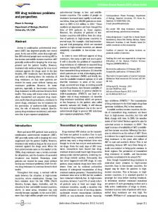
acid receives information about all other amino acids to the right and those to the left. For this reason it is necessary to use a noncausal network (Baldi et al. 2000). Another factor that is important for the selection of the learning method is that we are working with mutated sequences. A sequence can mutate in three ways: a simple change of amino acid (i.e. one amino acid is replaced by another one), an insertion, or a deletion of an amino acid. In the first case, the length of the sequence does not change, but in the other two cases it does. To solve this problem we need a method that allows a dynamic input. Recurrent neural networks were originally created to analyze time series in which the present moment is influenced by the past and the future (Tsoi and Back 1997). We used them here to analyze one-dimensional spatial sequences but the idea is essentially similar. For the reasons discussed above we decided to use a neural network topology where the sequence is analyzed in three parts with identical length (the most simple topology in the BRNR), so that the processing of the middle part is influenced by the first and third part. Simultaneously, these extreme parts are influenced by the middle. In this way the training of the network represents the nature of the problem a little better. There are several topologies for recurrent networks that have been used in the literature to solve different problems. A bidirectional dynamic topology is described and used for prediction of secondary structures by Baldi (Baldi and Soren 2001; Baldi 2002). We based our work on a similar topology of bidirectional dynamic networks, as another learning method to solve the problem. Figure 1 shows an example of this topology for our problem. The network has 33 input neurons and 2 output neurons. It has context layers backward (HB), forward (HF) and the hidden layer (HO). In other words, this topology consists of two context blocks, one of them with recurrence to the left and another one with recurrence to the right. For each sequence we refer to s as the middle part, while we refer to left as the information received from layer HB (subsequence “s-1”) and right as the information received from layer HF (subsequence “s+1”). But it should be noted that s is also considered the “right part” of the sequence s-1 and the “left part” of sequence s+1. To HB and HF we developed several tests always assigning the same weight to the pattern from the previous subsequence and to the pattern from the posterior subsequence, according to the given drug. Table 1 shows the numbers of neurons of the topology with which we obtained the best results. In this case the 33 inputs are real values and the outputs are (0,1) or (1,0), meaning resistant and susceptible, respectively. A classification problem is not the typical problem to solve in this kind of network. We do not have an output associated with each subsequence. But we considered the three parts of a sequence associated with the same output. Specifically the sequence was divided in three parts, that is, 33 inputs in each part and three outputs- one output for each part. As training algorithm of this network, the Backpropagation Through Time (BPTT) was used (Werbos, P. J. 1990). As target function we used Cross-Entropy and as output activation function we used a Softmax function.
… q-1
…
HO
HB
q+1
…
…
HF
… 33
Fig 1. Bidirectional Recurrent Neuronal Network Topology. Each of the arrows from layer to layer means that there are connections of all the neurons of the origin layer with all the neurons of the destination layer. The discontinuous arrows represent the connections between the parts, the shift operator q+1 means that the connection is from a left immediate part, and the shift operator q-1 means that the connection comes from the right immediate part.
2.5
Performance measures
There are several measures to evaluate the prediction performance. Most of the results previously reported in the literature are evaluated with the standard accuracy measure, defined as
Accuracy =
TP + TN TP + TN + FP + FN
(1)
where TP, TN, FP and FN are the number of true positive, true negative, false positives and false negatives, respectively. For this reason we used this measure in order to evaluate our results. We also used the measure performance of Sensitivity (Se) and Specificity (Sp) defined as Se =
TP TP + FN
Sp =
TN TN + FP
(2) (3)
Table 1. Number of neurons associated to the context layers backward (HB), forward (HF) and to the hidden layer (HO) for each neuronal network
Drug
HB=HF
HO
SQV
11
11
LPV
11
11
RTV
20
20
APV
20
20
IDV
27
20
ATV
32
32
NFV
20
20
To evaluate the results, k-fold cross-validation was applied to the dataset. This method is based on dividing the data in k ran-
3
dom subsets and to use one of the k subsets as the test set and to combine the other k-1 subsets to form a training set. This is repeated k times. Then the average error across all k trials is computed.
3
Table 3. Classification performance of SVM variants using Energy.
polynomial Radial
RESULTS
As explained above, we used three different methods (SVM, MLP and BRNN) to predict resistance of HIV sequences using seven inhibitors. We compared the results with those published previously (Beerenwinkel, N. et al. 2002; James, R. 2004). All results were averaged using 10-fold cross-validation. We used MLP to compare with the results obtained up to now to demonstrate that the Energy as well as ∆Energy are adequate feature representations for the resistance prediction. Table 2 shows that the results of MLP with Energy are quite similar to those of the ∆Energy. Both are similar to the previous results. Table 2. Prediction performance of methods used before: KNN, several decision trees and the prediction performance using MLP. Prediction performance is measured in terms of accuracy.
1
2
3
4
New
5
6
MLP
MLP
Drug
KNN
Dtree
DTree
Dtree*
Energy
∆Energy
SQV
81.7
80
85.7
87.5
85.47
87.88
LPV
81.1
92.33
87.88
RTV
82
90.92
90.71
89.5 89
89.5
89.8
APV
80.9
75.8
75.8
87.4
82.17
80.65
IDV
80.6
85
85.5
89.1
86.96
92.55
80.00
74.16
86.63
87.13
ATV NFV
73.6
91.8
93.7
88.5
The columns 1, 2 and 3 correspond to the results reported by James (2004) using KNN, the classic decision tree using ID3 and a variant of a decision tree developed respectively. The column 4 represents the results obtained by Beerenwinkel et al. (2002) using a classic decision tree. *Note the results of classical decision trees by James are different than those of Beerenwinkel due to a different number of cases; Beerenwinkel et al. used more cases to decision tree training. The columns 5 and 6 show our results using a MLP.
The other technique used was SVM with both Energy and
∆Energy. Table 3 shows the results obtained with the variant of Energy for linear SVM, using linear kernel, polynomial of degree 1 (other variant of linear), degree 2, degree 3, and radial basis. For the representation using ∆Energy these variants of SVM gave similar results.
4
Drug
linear
degree 1
degree 2
degree 3
Basis
SQV
87.82
80.82
69.68
85.23
82.38
LPV
88.57
85.14
85.14
88.57
85.14
RTV
91.83
84.96
79.08
92.15
86.92
APV
82.30
77.47
77.47
83.64
78.82
IDV
91.51
86.73
83.81
92.57
88.59
ATV
74.38
71.07
68.59
72.72
70.24
NFV
84.86
75.68
70.96
84.86
80.14
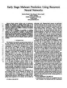
After analyzing these results we can see that the feature representation using Energy as well as the representation using ∆Energy are appropriate to describe the sequence in this task. As explained earlier, we used BRNN to solve the problem. The network has three output values during the predicting process, that is, the output is a vector with three components, because an output is obtained for each part. As in the other techniques used, we represent the output with the two values explained before - resistance and susceptible-. The difference with regard to the other methods is that, now we will have three outputs in the prediction. The BPTT algorithm is based on the unfolding and folding process. For each case in the training dataset, in the forward process the network is unfolding as a classical feedforward network and executes the Backpropagation algorithm to obtain the corresponding output as is shown in Figure 2. In the backward process the network is folding again to turn back as the beginning (Fig. 1) in order to update the weights (Werbos 1990). As is illustrated in Figure 2, we split the instances in the database. Figure 2 shows the first step to the BPTT and the processing of the outputs in order to use this network in this classification problem. The prediction is divided in three tasks. The first task is to split the sequence in three parts, representing the three entries to parts the network. The second task is to unfold the network and to obtain the three outputs for this input, and the third task is to compute the final output - to represent the resistance or not of this protein - as an adequate combination of the three previous outputs. In our training dataset we represented the class in the three outputs (output 1, output 2, output3) using the same value, that means, 1 for resistance and 0 for susceptible. But in the prediction we can obtain different outputs for each part, i.e. the output is a vector of three coordinates: (O1, O2, O3), where Oi є {0, 1}
using Recurrent Neural Networks
Output=Mode (outputt-1, outputt, outputt+1) or Output=outputt
Output Processing output 3
s+1 …
…
…
…
output 2
s …
…
…
… output 1
s-
…
… …
(AA1…AA33)
Protease Sequence
(AA34 … AA66)
(AA67 … AA99)
AA1, AA2,…, AA33, AA34, AA35,…, AA66, AA67, AA68…AA99
Fig 2. Bidirectional Recurrent Neuronal Network Unfolding
5
Table 4. Classification performance using bidirectional recurrent neural networks.
Table 5. Sensitivity and Specificity of the MLP and a BRNN variant. MLP
BRR
BRNN
Drug
(mode)
(middle output)
SQV
91.16
91.16
LPV
94.42
94.39
RTV
93.42
94.73
APV
89.25
88.71
IDV
92.55
92.55
ATV
82.67
81.33
NFV
94.06
93.07
Now the problem is the following: once the network has finished its prediction and we have its vectorial output, we need to select one of its components as the sole final output. Several variants can be designed to obtain one output from the three outputs. In this paper we will deal with two of them as is shown in the Figure 2. A first output variant is the mode of the three outputs and a second variant is the output corresponding to the middle time (output from time t=2). In the case of the first variant we are obtaining the value that is more frequent at the three parts and that gives the same weight to all parts of the sequence. In the second case it is valid to remember that this middle output was influenced by the other two parts. For this reason it presumably has more information about the whole sequence than the other ones. For this method we took as feature values the ∆Energy. The results are shown in Table 4. Similar results were obtained using the selection variant of the mode of the three outputs as well as the variant using the output of the middle time. We also used statistical methods to analyze the results. A Friedman two-way ANOVA test was used to compare the results of Table 2 in order to validate the accuracy of the MLP. This test showed that there are significant differences between the methods. The Friedman test demonstrated that methods 3 and 5 (as referred in Table 2) are better than the rest. A Wilcoxon test ratified that these two algorithms (3 and 5) are similar. A Friedman two-way ANOVA test was also used to compare the different SVM used in this work (shown in Table 3) and a Wilcoxon test was applied to compare with the results obtained by other authors (reported in Table 2). With these tests we do not obtain significant differences between the results of these algorithms. We proceeded in the same way with the RNN. We compared the results of this method with the best result in previous works, and with the best result using MLP. The statistical tests yielded significant differences between the accuracy of these techniques. We used these statistics also to compare the two different kinds of final output processing (mode and middle output). In this case we demonstrated that the results of both BRNN are an appropriated method to the problem, because the accuracy is greater than or similar to the rest.
Drug
sensitivity
BRNN (middle output) specificity
sensitivity
specificity
SQV
84.70
90.57
90.48
92.59
LPV
84.70
90.57
96.25
77.78
RTV
88.41
94.52
89.74
100
APV
80.95
80.39
84.81
87.85
IDV
95.72
89.36
95.35
90.2
ATV
78.53
73.33
87.5
80
NFV
89.37
79.31
94.44
89.66
In addition we compared, in the same way, the specificity and sensitivity of all methods used. In this case the results were different for the different drugs. In general the results of BRNN are good but we do not obtain better results regarding the specificity of APV and LPV with regard to KNN used by James (2004). The results of these tests can be found as supplementary information.
4
CONCLUSIONS
In this paper we analyzed a recurrent neural network with an appropriate topology to analyze sequences in classification problems. In particular, we studied the problem to predict the Human Immunodeficiency Virus Drug Resistance. Amino acid energies of the Protease were used as features to represent the sequence with characteristics related to their 3D structure. A comparative evaluation of a selection of machine learning algorithms was performed, demonstrating the reliability of both the use of energy as features and the use of recurrent neural network as predictors. It was demonstrated that both Energy (amino acids contact energy) and ∆Energy (difference of the amino acid energy in a mutant sequence with respect to wild type) are good features to represent the HIV genotype, and the results obtained were similar and in some cases better than other features used so far. It was demonstrated that the BRNN could be used as a classification method for this problem. Prediction performance obtained was greater than or at least comparable with results obtained previously. The accuracy was between 81.4% and 94.7%. The two variants of networks output computation were averaged using 10-fold cross-validation and had similar results, concluding that both can be used in this problem. For the output selection variant, values of specificity and sensitivity were obtained between 74.1-100% and 77.5-95.8% respectively. In the selection variant using the mode the results of sensitivity and specificity were 84.8-96.2% and 77.7-100% respectively.
ACKNOWLEDGEMENTS This work was developed in the framework of a collaboration program supported by VLIR (Vlaamse InterUniversitaire Raad, Flemish Interuniversity Council, Belgium).
6
using Recurrent Neural Networks
REFERENCES Baldi, P. (2002). New Machine Learning Methods for the Prediction of Protein Topologies, In: P. Frasconi and R. Shamir (eds.) Artificial Intelligence and Heuristic Methods for Bioinformatics, IOS Press. Baldi, P., et al. (2000). "Bidirectional Dynamics for Protein Secondary Structure Prediction." In: R. Sun and C.L. Gile (eds.) Sequence Learning, LNAI 1828: 80-104. Baldi, P. and Soren, B. (2001). Bioinformatics: The Machine Learning Approach., MIT Press. Beerenwinkel, N., et al. (2003). "Geno2pheno: estimating phenotypic drug resistance from HIV-1 genotypes." Nucl. Acids Res. 31(13): 3850-3855. Beerenwinkel, N., et al. (2002). "Diversity and complexity of HIV-1 drug resistance: A bioinformatics approach to predicting phenotype from genotype." PNAS 99(12): 8271-8276. Bonet, I., et al. (2002). "Learning optimization in a MLP Neural Network Applied to OCR." MICAI 2002: Advances in Artificial Intelligence. LNAI 2313: 292-300. Cao, Z. W., et al. (2005). "Computer prediction of drug resistance mutations in proteins." Drug Discovery Today 10(7): 521-529. James, R. (2004). Predicting Human Immunodeficiency Virus Type 1 Drug Resistance from Genotype Using Machine Learning. MSc Thesis University of Edinburgh Miyazawa, S. and Jernigan, R. L. (1994). "Protein stability for single substitution mutants and the extent of local compactness in the denatured state." Protein Eng. 7: 1209-1220. Miyazawa, S. and Jernigan, R. L. (1996). "Residue Potentials with a Favorable Contact Pair Term and an Unfavorable High Packing Density Term, for Simulation and Threading." J. Mol. Biol. 256: 623-644. Rabinowitz, M., et al. (2006). "Accurate prediction of HIV-1 drug response from the reverse transcriptase and protease amino acid sequences using sparse models created by convex optimization." Bioinformatics 22(5): 541-549. Rumelhart, D. E., et al. (1986). Learning internal representations by error propagation, MIT Press. Parallel distributed processing: explorations in the microstructure of cognition, vol. 1: foundations: 318-362. Scmidt, B., et al. (2000). "Simple algorithm derived from a geno-/phenotypic database to predict HIV-1 protease inhibitor resistance." AIDS 14: 1731-1738. Sevin, A. D., et al. (2000). "Methods for investigation of the relationship between drug-susceptibility phenotype and human immunodeficiency virus type 1 genotype with applications to AIDS Clinical Trials Group 333." Journal Of Infectious Diseases 182(1): 59-67. Tsoi, A. and Back, A. (1997). "Discrete time recurrent neural network architectures: A unifying review." Neurocomputing 15: 183-223. Wang, D. C. and Larder, B. (2003). "Enhanced prediction of lopinavir resistance from genotype by use of artificial neural networks." Journal Of Infectious Diseases 188(5): 653-660. Werbos, P. J. (1990). Backpropagation Through Time: What it does and How to do it, IEEE.
7