In this paper, we deal with the problem of categoriz- ing different underwater habitat types. Previous works on solving this categorization problem are mostly ...
2013 IEEE International Conference on Computer Vision Workshops
Categorization of Underwater Habitats Using Dynamic Video Textures Jun Hu1 , Han Zhang1 , Anastasia Miliou2 , Thodoris Tsimpidis2 , Hazel Thornton2 , Vladimir Pavlovic1 1 Department of Computer Science, Rutgers University, Piscataway, NJ 08854, USA 2 Archipelagos Institute Of Marine Conservation, Pythagorio, Samos 83102, Greece {jh900,han.zhang,vladimir}@cs.rutgers.edu {a.miliou,t.tsimpidis,hazel}@archipelago.gr
Abstract In this paper, we deal with the problem of categorizing different underwater habitat types. Previous works on solving this categorization problem are mostly based on the analysis of underwater images. In our work, we design a system capable of categorizing underwater habitats based on underwater video content analysis since the temporally correlated information may make contribution to the categorization task. However, the task is very challenging since the underwater scene in the video is continuously varying because of the changing scene and surface conditions, lighting, and the viewpoint. To that end, we investigate the utility of two approaches to underwater video classification: the common spatio-temporal interest points (STIPs) and the video texture dynamic systems, where we model the underwater footage using dynamic textures and construct a categorization framework using the approach of the Bag-ofSystems(BoSs). We also introduce a new underwater video data set, which is composed of more than 100 hours of annotated video sequences. Our results indicate that, for the underwater habitat identification, the dynamic texture approach has multiple benefits over the traditional STIPbased video modeling.
Figure 1. Visual images captured via a high resolution underwater cartographic HD camera
Many recent works on underwater object or scene classification are based upon the analysis of images collected by underwater visual sensors [6, 9, 7, 11]. In our work, the classification problem is faced by exploiting theories and techniques provided by underwater video analysis since the temporally correlated visual information may make contribution to distinguish different kind of habitats. Obtaining compelling visual categorization result on the underwater video footage can be a difficult task for two reasons. Firstly, systematically describing distinction among various habitat types from a video set, such as the scenes in Figure 1, is often challenging for experts themselves because of simultaneous occurrence of multiple and uncertain habitat identifiers, such as the types or the density of seagrass. Secondly, although several detectors and descriptors [8, 3, 13] have shown strong results in modeling space-time video sequences, especially in tasks such as object and action recognition problems, the state-of-the-art approaches
1. Introduction Recent years have witnessed an incredible growth of marine economy. However, with the increasing human activities, the stability of marine ecosystems is facing severe threats due to pollution, overfishing, exploitation of underwater sources, etc. Hence, a system with the function of monitoring and analyzing the change and damage of the marine environment would be highly advantageous in the monitoring and protection of this invaluable habitat. In this paper, we design a system capable of categorizing different underwater habitat types. With the help of this system, one will be able to build detailed maps of different ecosystems and then identify the degree of destruction to the marine environment. 978-0-7695-5161-6/13 $31.00 © 2013 IEEE 978-1-4799-3022-7/13 DOI 10.1109/ICCVW.2013.115
838
have poor performance in our scenario since the underwater scene is continuously varying in the appearance, illumination, artifacts from surface deformations (waves), light scatter, as well as the viewpoints of camera by which the video sequences were taken. Last but not the least, the sparseness of annotated observation data and shortage of relevant references on underwater video categorization problem make this task challenging beyond typical visual sequence categorization problems. Most recent approaches to video content analysis have focused on identification of space-time interest points. In [8], Laptev and Lindeberg proposed the Harris3D detector, which compute a spatiotemporal second-moment matrix at each video point using independent spatial and temporal values. The HOG/HOF introduced in [8] was utilized to describe the character in the selected interest points. Another detector was proposed by Dollar in [3], which is based on temporal Gabor filters and a 2D spatial Gaussian smoothing kernel. Interest points are selected as local maxima and then described by Cuboid descriptor, which concatenates on the computing of local gradients for each pixel in a patch centered at each interest point. Willems proposed Hessian detector [13] as a spatiotemporal extension of the Hessian saliency measure. All these works have shown great success for many spatiotemporal video content recognition tasks such as object and scene recognition. However, all the above approaches are based on local interest points extraction, and this property makes it unreasonable to utilize these detectors and descriptors in our problem because, in our case, we are interested in the motion of the whole underwater scene where every point may contribute to identification of the scene. As a result, we seek to describe patches instead of specific interest points. Dynamic texture related approaches [4, 12, 1] perform very well in modeling and synthesizing space-time video patches. Dynamic textures are sequences of images of moving scenes that exhibit certain stationary properties in time, such as the water on the surface of a lake, the flag fluttering in the wind, etc. Among several strongly performing approaches, Doretto’s [4] use of linear dynamic systems(LDSs) shows good generalization properties and robustness to scene artifacts. In this paper, we focus on using Linear Dynamic Systems to model underwater scenes and then categorize them into different habitat types. In order to make the variation of viewpoints in the underwater video have less impact on the categorization precision, we model video sequences as Bag-of-Systems(BoSs), inspired by the Bag-of-Feature(BoF) approach [10], where an image is hypothesized to be identifiable by the distribution of certain key features extracted from the image. Hence, a video sequence can be represented by the distribution of LDSs. However, traditional classifiers, such as Nearest Neighbors and Support Vector Machines(SVMs) will
not work if the original non-Euclidean distance between LDSs is selected as the distance metrics. We need to define an indirect distance between two LDSs. In our work, we calculate the Martin distance [2] as the metric distance between two LDSs. Finally, by testing different settings for the BoSs on our Posidonia Oceanica underwater video set, we study the impact of different framework factors on the habitat categorization task. In this paper, we deal with the problem of categorizing different underwater habitat types. Our first contribution is making use of the temporal information in the video to categorize underwater habitats, rather than just isolated images. We also introduce a new annotated underwater video data set, which is composed of more than 100 hours of annotated video sequences taken by a high resolution underwater cartographic HD camera.
2. Preliminaries We firstly introduce necessary concepts that are required to understand our approach. We introduce Linear Dynamic Modeling and Martin distance between LDSs in this section.
2.1. Linear Dynamic System Given a video sequence {y(t)}F t=1 , we can model it as the output of LDS as x(t + 1) = Ax(t) + v(t)
v(t) ∼ N (0, Q)
(1)
y(t) = C0 + Cx(t) + w(t)
w(t) ∼ N (0, R)
(2)
where x(t) is a hidden state at time t, A ∈ Rn×n models the dynamics of the system, and C ∈ Rm×n maps from the hidden state to the output of the system. C0 is the mean of the video sequence. And v(t) ∼ N (0, Q), w(t) ∼ N (0, R) represent the measurement and processing noise. n is the order of the LDS system, and m is number of pixels in one frame of a video sequence. This model decouples the dynamics of the system, which is modeled by A, from the appearance, which is modeled by C. Therefore, we can describe a given spatiotemporal patch using a tuple M = (A, C). Such a feature descriptor models both the dynamics and appearance in the spatiotemporal patch as opposed to image gradient that only models local texture. To calculate the parameters of this dynamic system, Doretto et al. [4] introduced a fast but suboptimal method for identifying the system coefficients. It is suboptimal since when calculate the hidden state x(t), the equation 1 is not enforced. The basic calculation is based on the Principal Component Analysis(PCA) and the Singular value decomposition(SVD). 839
Systems framework can be concluded as:(1) extracting dynamic textures in underwater video footage and then describe them using LDS. (2) Clustering methods, such as Kmeans, hierarchial clustering, are utilized on the extracted LDSs and then cluster centers are selected as codewords. (3) Using this codebook, we can assign labels to the LDSs, so each video sequence can be represented by the distribution of codewords. (4) Compare the distribution of codewords from a query video sequence with video sequences in the database, and then infer its category by the knowledge from training set.
3.1. Feature Extraction and Description There are two popular approaches in extracting features: interest points approach and dense sampling. For interest points approach, certain pixels are selected as ”interesting”. This kind of points show a salient property matching certain requirements, such as certain extreme conditions on shape, intensity, optical flow or gradients of neighborhoods around them. For dense sampling, fixed size patches or volumes are extracted and described. In our scenario, it is reasonable to use dense sampling since we are interested in the motion of the whole underwater scene where every point may contribute to identification of the scene. After dividing video sequences into volumes, we model each volume using Linear Dynamic System and calculate coefficients for this system. After that, every video volume can be represented by a tuple M = (A, C) as the descriptor. Such descriptor models both the dynamics and the appearance in a spatiotemporal patch as opposed to gradients that only model local texture.
Figure 2. Framework of the machine learning system
2.2. Martin Distance Between LDSs Since the classifiers do not work if the original nonEuclidean distance between LDSs is the distance metrics, we need to introduce an indirect distance metrics. In [2], the proposed Martin distance is one effective approach. The distance between two LDSs is based on subspace angles. Given the tuple M = (A, C), the angle is defined in observability subspace, represented as O∞ (M ) = [C � , (CA)� , (CA2 )� , ...]� ∈ (R)∞×n . The angle distance is calculated by solving the Lyapunov equation A� PA − P = −C � C for P, where � � P11 P12 P= ∈ R2n×2n (3) P21 P22 � A= C=
�
0 A2
A1 0
C2
C1
� �
3.2. Codebook Formation
∈ R2n×2n
(4)
∈ Rm×2n
(5)
After extracting features from the whole training set, we get {Mi = (Ai , Ci )}Ti=1 , where T represents the total number of features. Then the Martin distance is utilized to map the none-Euclidean distance between two LDSs to Euclidean space. To reduce computational cost in clustering process, we firstly embed the LDSs from high order to low dimension space. We compute the pairwise Martin distance matrix D ∈ Rl , where l is the dimension of embedding, such that Dij = d(Mi , Mj ). After that, Multidimensional Scaling(MDS) works with pairwise distances matrix to make dimensional reduction. When the MDS procedure is done, we get low dimensional points {Wi }Ti=1 , which are all in Euclidean space. All these points correspond to the LDSs in high dimensional space respectively, which means Wi and Mi are one-to-one correspondence for all i from 1 to T . Then, K-means clustering method is applied to {Wi }Ti=1 . After clustering, we have K cluster centers {ki }K i=1 . However, this cluster centers do not correspond to the original space LDSs. In order to form our codewords {Zi }K i=1 , we find the LDSs whose corresponding words in low di-
The cosine of the subspace angles {θi }ni=1 is calculated as −1 −1 cos2 θi = ith eigenvalue(P11 P12 P22 P21 )
(6)
With the angles, the Martin distance can be calculated by 2
dM (M1 , M2 ) = −ln
n �
cos2 θi
(7)
i=1
However, there is one limitation of Martin distance that the number of the output pixels for both of the Linear dynamic systems needs to be the same. This limitation can be solved by resample and resize the video size. More detailed discussion can be found in [2].
3. Proposed System Framework and Methods Basic system framework is described in Figure 2. Inspired by the Bag-of-Features approach, our Bag-of840
mension space has the least distance to the cluster centers, such that Zi = Mb ,
b = argmin � Wj − Ki �
2
j
(8)
In this way, we get our codebook Z = {Z1 , Z2 , ..., ZK }, where Zi = (Ai , Ci ).
3.3. Video Representation
(a) C1: healthy and dense oceani- (b) C2: patchy oceanica seagrass ca seagrass
Once the codebook is formed, every video sequence can be represented by a histogram H = [h1 , h2 , h3 , ..., hK , l], where hi is a weight value of the ith codeword in the video sequence, l is the class label of the video sequence. The label l has been assigned by professionals before the experiment. To calculate hi , the easiest way is to calculate the count of occurrence of the ith codeword. More sophisticated ways are the Term Frequency defined by equation 9 and the Term Frequency Inverse Document Frequency (TF-IDF) defined by equation 10. cik hik = �K
k=1 cik
, k = 1, ..., K and i = 1, ..., N
cik hik = ( �K
k=1 cik
)ln(
N ) Nk
(c) C3: sandy and muddy substrate
Figure 3. Sample snapshots from underwater scenes
(9)
4. Experiment and Results
(10)
The purpose of our work is to investigate feasible approaches to categorize underwater scenes into different habitat types. In our experiment, we compare the performance of the space-time interesting points(STIPs)-based approach with the dynamic textures-based approach on our video set. In order to test the effectiveness of the Bag-ofSystem approach, we compare the performance of the BoSs with the single LDS approach. In particular, we investigate the impact of the volume size of dense sampling and alternative experimental choices for the BoSs, such as TF-IDF versus TF weights, as well as the role of classifiers, SVM versus K-NN, on the categorization performance.
where N is the total number of video sequences in the video set, Nk is the number of video sequences in which codeword k appears at least once, cik represents codeword k appears cik times in the ith video sequence, hik is the weight of codeword k in the ith video sequence. Once a histogram H is computed, we normalize it by its L1 norm.
3.4. Classification Given the training set, we can model video sequences as {(hi , li )}N i=1 , where hi is a histogram extracted from ith video sequence and li is the class label assigned. The classification problem can be concluded as given a query histogram h, infer the class label for this histogram. One simple approach to obtain the label is to use the k-nearest neighbors(k-NN) classifier [5], where query video sequence is assigned the majority class label of its k closest histograms from the training database. Another approach is to use a discriminative classification method like kernel SVM. The effectiveness of these two classifiers is compared in our experiment. To calculate the distance between two histogram, we use the χ2 distance, which is define as
4.1. Data Set The underwater video data set is provided by Archipelagos, Institute of Marine Conservation. Approximately 100 hours of video footage was recorded via a high resolution underwater cartographic HD camera, visualizing the benthic habitat of Posidonia oceanica seagrass meadows in the Aegean Sea of the Mediterranean Sea. The endemic seagrass species forms extensive meadows which extend from intertidal zones to depths of 50-60m and are estimated to colonize between 25,000 and 45,000 km2 of the Mediterranean basin. Video sequences were taken from different viewpoint and scales, with various noises(e.g. subtitles and floating of the mobile camera), causing increased difficulty in categorization.. We select relatively representative annotations from our
K
dχ2 (h1 , h2 ) =
1 � |h1k − h2k |2 2 h1k + h2k
(11)
k=1
where hik denotes the kth element of the histogram vector hi . 841
Approach STIPs single LDS 2×2 4×4
to get enough points, we lower down the threshold of confidence which represents the degree of space-time saliency and do categorization by the Bag-of-Feature approach. Result is shown in table 1. It is very obvious that dynamic textures-based approach has better performance. In our scenario, the STIPs-based approach fails to get compelling result since we are interested in the motion of the whole scene in which every point may contribute to the identification of the scene. 3)Effectiveness of Bag-of-System and Dense Sampling. We compare the performance of the single LDS approach with the BoSs approach and investigate the impact of the size of dense sampling. For the single LDS approach, no BoSs method is utilized for categorization. Given a test video sequence, the Martin distance between the testing LDS and LDSs in the training set is firstly calculated and then the label of its nearest neighbor is chosen as the label for this video sequence. For the BoSs approach, we vary the dense sampling volume size by dividing the 720 × 360 video sequence into 2 × 2 , 4 × 4 spatial cells, and the size in temporal direction is not changed and then model each cell as a LDS. We introduce TF-IDF representation for each video and finally use K-NN classifer with k=1 to do the classification. The overall result is shown in table 1. As the result shows, the BoS approach performs more effectively than the Single LDS approach. In the meanwhile, it shows that the dense sampling size is a crucial factor to overall performance. In our experiment, we do not do the optimization work on the cell size. Table 2 depicts a confusion matrix of the BoS approach when we select 4 × 4 spatial cells (in the following analysis, all the results are based on this size setting). The entry value is the ratio of the column class label in the result while its actual class label should be the row index(e.g. 0.11 means that when we have 100 test video sequences whose actual class label is C1 but 11 of them are assigned class label C2 in the experiment). The result is reasonable since it is easier to mix up healthy grass with patch grass than confuse it with the barren muddy surface. 4)Representation and Classification: As mentioned above, we choose k = 1 in the k-NN classifier and we use radial basis kernel in the SVM classifier. In addition, since our data set is relatively small, we did not use crossvalidation to tune the parameters in the classifiers. Table 3 displays the categorization performance against the choice of classifiers and representations. Figure 4 gives a more detailed performance demonstration on the effect of representations and classifiers as a function of the codebook size from 3 to 12. We can see that the k-NN classifier performs a little better than the SVM classifier(less than 10% in table 3). In addition, the choice of the representation has little effect on the overall result(less than 5%). We can verify the
Truth 0.40 0.63 0.78 0.88
Table 1. Average Categorization Performance for different approaches
C1 C2 C3
C1 0.89 0.17 0.07
C2 0.11 0.83 0.00
C3 0 0 0.93
Table 2. Confusion matrix of BoS for approach(4 × 4).
date set, which contains 3 major underwater habitat types: (C1) healthy and dense oceanica seagrass; (C2) patchy oceanica seagrass; (C3) sandy and muddy substrate. Figure 3 shows some sample frames from this database. For each class, we extract 80 video subsequences from the whole video sequences, and each of the video subsequence is of size 720 × 480 × 3, which 720(pixels) and 480(pixels) are the scale of video frames and 3(seconds) is the length for each video clip. Our experiment is conducted on the middle portion in the video of size 720 × 360. We cut off the top and bottom part since they are covered by noisy information like the subtitles describing the time, depth and coordinates.
4.2. Implementation Details And Quantitative Comparisons 1)Training and Validation. In the experiment, the method we use to test the effectiveness of our approach is cross-validation. Given the dataset composed of 240 labeled video subsequences(80 for each class), we divide it into two parts as training and validation sets. We train our model on 192 randomly picked samples(64 from each class), and test the truth on the validation set left. 2)STIPs and Dynamic Textures. We firstly test the performance of space-time interest points(STIPs)-based approach. This approach seeks to find space-time salient points in video sequences and then do categorization based on these ”interesting” points. In our experiment, we only extract 16 salient points within a 3-second video subsequence using the code from Ivan Laptev’s website1 by default setting. The STIPs are sparse because our video sequences show a stationary property of moving scenes. Within continuous frames, the change of objects or scenes is very slow and smooth, which makes the STIPs detector hard to recognize local space-time salient points. In order 1 http://www.irisa.fr/vista/Equipe/People/Laptev/download.html#stip
842
Method SVM + TF SVM + TF-IDF k-NN + TF k-NN + TF-IDF
the experimental data set. Additional experimental factors such as the optimization of patch and segmentation size, codebook size should be investigated. Moreover, it will be interesting to try the generalised bag-of-features techniques, such as spare coding for classification introduced in [14], to compare its performance with BoSs.From the perspective of methodology, we can combine the isolated image textural analysis with temporal information and also combine STIPs with dynamic textures to do classification. Another interesting issue is to investigate other dynamic systems(e.g. kernel dynamic systems) to model the dynamic textures.
Average Performance 0.8333 0.8095 0.8667 0.8852
Table 3. Average Categorization Performance of SVM and k-NN with TF and TF-IDF representation
References [1] Z. Bar-Joseph, R. El-Yaniv, D. Lischinski, and M. Werman. Texture mixing and texture movie synthesis using statistical learning. IEEE Trans. Vis. Comput. Graph., 7(2):120–135, 2001. [2] A. B. Chan and N. Vasconcelos. Classifying video with kernel dynamic textures. In CVPR, 2007. [3] P. Doll´ar, V. Rabaud, G. Cottrell, and S. Belongie. Behavior recognition via sparse spatio-temporal features. In Visual Surveillance and Performance Evaluation of Tracking and Surveillance, 2005. 2nd Joint IEEE International Workshop on, pages 65–72. IEEE, 2005. [4] G. Doretto, A. Chiuso, Y. N. Wu, and S. Soatto. Dynamic textures. International Journal of Computer Vision, 51(2):91–109, 2003. [5] R. O. Duda, P. E. Hart, and D. G. Stork. Pattern classification. John Wiley & Sons, 2012. [6] A. Friedman, D. Steinberg, O. Pizarro, and S. B. Williams. Active learning using a variational dirichlet process model for pre-clustering and classification of underwater stereo imagery. In IROS, pages 1533–1539, 2011. [7] G. A. Hollinger, U. Mitra, and G. S. Sukhatme. Active classification: Theory and application to underwater inspection. CoRR, abs/1106.5829, 2011. [8] I. Laptev and T. Lindeberg. Space-time interest points. In ICCV, pages 432–439, 2003. [9] N. Nandhakumar and S. Malik. Multisensor integration for underwater scene classification. Appl. Intell., 5(3):207–216, 1995. [10] J. Sivic and A. Zisserman. Video google: A text retrieval approach to object matching in videos. In ICCV, pages 1470– 1477, 2003. [11] D. Steinberg, S. B. Williams, O. Pizarro, and M. V. Jakuba. Towards autonomous habitat classification using gaussian mixture models. In IROS, pages 4424–4431, 2010. [12] M. Szummer and R. W. Picard. Temporal texture modeling. In Image Processing, 1996. Proceedings., International Conference on, volume 3, pages 823–826. IEEE, 1996. [13] G. Willems, T. Tuytelaars, and L. J. V. Gool. An efficient dense and scale-invariant spatio-temporal interest point detector. In ECCV (2), pages 650–663, 2008. [14] J. Yang, K. Yu, Y. Gong, and T. S. Huang. Linear spatial pyramid matching using sparse coding for image classification. In CVPR, pages 1794–1801, 2009.
Figure 4. Categorization performance of BoS as a function of the codebook size.
above conclusion using the result in figure 4. The figure also shows that the performance of classifiers is consistent with the scale of codebook size. Consequently, considering the scale of our data set, the performance of different classifiers and representations is not necessarily statistically significant. Our framework is not particularly dependent on the choice of the representation and the classifier.
5. Conclusion and Future Work In this paper, we proposed a machine learning system capable of categorizing different habit types. Most of previous works for categorizing underwater objects and scenes are based on the analysis of isolated images. We investigated a new approach to make use of temporal information in underwater video sequences for categorization. This task is very challenging because the underwater scene is continuously changing in the appearance, illumination, artifacts from surface deformations (waves), light scatter, as well as the viewpoints. According to the property of underwater video sequences, we selected dynamic textures and construct the whole framework by the approach of the Bagof-Systems. The experimental results show that our BoS system is feasible and effective to do categorization on our video data, in contrast to the more common STIP video representations that fail to provide appropriate descriptors for our underwater video scenes. In our experiment, we only use small part of video sequences, which has relatively representative features and is less noisy than other video sequences. But in reality, most of video footage is more complex and there are much more underwater habitat types. In the future, we need to expand 843