A Density-based Cluster Validity Approach using Multi-representatives Maria Halkidi∗,
Michalis Vazirgiannis
Department of Informatics, Athens University of Economics & Business 76 Patision Street, Athens 104 34, GREECE Email:
[email protected], mvazirg@ aueb.gr
Abstract Although the goal of clustering is intuitively compelling and its notion arises in many fields, it is difficult to define a unified approach to address the clustering problem and thus diverse clustering algorithms abound in the research community. These algorithms, under different clustering assumptions, often lead to qualitatively different results. As a consequence the results of clustering algorithms (i.e. data set partitionings) need to be evaluated as regards their validity based on widely accepted criteria. In this paper a cluster validity index, CDbw, is proposed which assesses the compactness and separation of clusters defined by a clustering algorithm. The cluster validity index, given a data set and a set of clustering algorithms, enables: i) the selection of the input parameter values that lead an algorithm to the best possible partitioning of the data set, and ii) the selection of the algorithm that provides the best partitioning of the data set. CDbw handles efficiently arbitrarily shaped clusters by representing each cluster with a number of points rather than by a single representative point. A full implementation and experimental results confirm the reliability of the validity index showing also that its performance compares favourably to that of several others. Keywords: cluster validity, clustering, quality assessment, unsupervised learning
1. INTRODUCTION Since clustering is an unsupervised learning procedure and there is no a priori knowledge of data distribution in the underlying set, the significance of the clusters defined for a data set needs to be validated. Given a data set and a clustering algorithm running on it with different input parameter values, we obtain different partitionings of the data set into clusters. Then we need to select among the defined partitionings which one best fits the concerned data set. This, the cluster validity problem, is generally accepted as a cornerstone issue of the clustering process. However, the notion of “good” clustering is strictly related to the application domain and its specific requirements. Nevertheless it is generally accepted that the answer to the validity of the clustering results has to be sought in measures of separation among the clusters and cohesion within clusters. These are widely known as objective cluster validity criteria. To define these measures and evaluate clusters we have to take into account specific aspects of their definition. In this work we tackle the cluster validity problem based on the density properties of clusters. This implies that we measure the compactness and separation of clusters evaluating the density distribution within and between clusters. We define and evaluate a new validity index, CDbw (Composed Density between and within clusters) and a methodology that given a data set, S, and a set of algorithms A={algi} enables: i) finding the set of input parameter values that lead each algi to the best possible clustering results, and ii) taking into account the results of (i), finding algi that returns the best partitioning of S among those defined by the considered algorithms. There are cases that a clustering algorithm finds the correct number of clusters but partitions the data set in a wrong way (i.e. it fails to discover the real clusters into which the data can be organized).
∗
Corresponding author
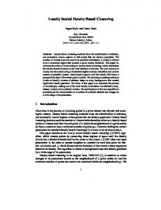
Figure 1: The different partitionings defined by K-Means when it runs with different input parameter values. Assuming different clustering algorithms’ sessions on a given data set (i.e. the application of the clustering algorithm to a data set using specific values for its input parameters), a set of different partitionings but all containing the correct number of clusters (that is, the number of clusters that present in the underlying data) is defined. CDbw enables finding the best partitioning of a data set among the aforementioned ones. Moreover, it adjusts well to non-spherical cluster geometries, contrary to the validity indices proposed in the literature (an overview is presented in [11]). It achieves this by considering multiple representative points per cluster. The cluster validity index is fully implemented and experiments prove its efficiency for various data sets and clustering algorithms. We note, here, that the cluster validity approaches can be considered to be a tool for assisting the user with the clustering process and they cannot be expected to solve all the problems related to the unsupervised learning. CDbw aims to assist with the evaluation of clustering results based on the criteria of the clusters’ well-separation and cohesion and the selection of the clustering that best approximates the clusters into which the given data can be organized. The users can exploit the results of the cluster validity and based on their requirements they could select the clustering that is suitable for their application domain. We note that our method finds the best partitioning among those that have been defined by the selected algorithm. Hence if the clustering algorithm does not manage to find the actual partitioning of a dataset then the cluster validity approach, of course, is not able to find the partitioning either. However it can be used to select among the defined clusterings, the one that mostly approximates the real clusters according to the requirement of well-separated and cohesive clusters. The rest of the paper is organized as follows. Section 2 motivates the definition of a new validity index and discusses some background information. Then, in Section 3 we present the fundamental concepts of our approach discussing also in detail the proposed cluster validity index. In Section 4 we describe an experimental study of our approach while we present its comparison to other cluster validity indices. In the sequel, Section 5 reviews cluster validity related concepts and some cluster validity criteria related to our work. Finally, we conclude in Section 6 by briefly presenting our contributions and indicating directions for further research.
2. PRELIMINARIES AND MOTIVATION OF THE CLUSTER VALIDITY APPROACH The validity assessment of clustering results is a complex problem and it depends on the application domain. In the sequel, we motivate the aspects of assessing the validity of clustering results, using examples. As Figure 1 depicts, a clustering algorithm (here, the K-Means [2] algorithm is used) with different input parameter values (for brevity, further referred to as ipvs) results in different clusterings. The data set is falsely partitioned in most of the cases. Only a specific set of ipvs (in this case when number of clusters = 3) lead to the actual partitioning of the data set. If there is no prior knowledge about the data structure, it is difficult to find the best ipvs for a given algorithm. Cross-algorithm comparison takes place in the example of Figure 6 where different clustering algorithms (K-Means [2], CURE [9], DBSCAN[6], a clustering algorithm provided by the CLUTO toolkit [17]) are used to partition the DS2 data set. The algorithms ran under specific set of ipvs to define a partitioning of DS2 into four clusters. As we can observe in Figure 6(a)-(c), K-Means, CURE (with ipvs a=0.3, r=10) and the CLUTO algorithm partition DS2 wrongly into four clusters. On the other hand, DBSCAN (see Figure 6(d)) with suitable ipvs gives better results since it partitions the data set discovering its real four clusters. A similar example is presented in Figure 7. Following up the examples discussed above, each algorithm provides a partitioning of a dataset but does not deal with the validity of the clustering results. They aim to find the best possible partitioning for the given ipvs but there is no indication that the defined clusters are the ones that best fit data.
Visual perception of the clusters structure enables a profound assessment of the partitioning validity. However, in case of large highdimensional data sets (e.g. more than three dimensions), effective visualization can be cumbersome. Moreover the perception of clusters based on visualization is a difficult task for humans not accustomed to higher dimensional spaces. What is then needed is a visual-aids-free assessment of some objective criterion, indicating the validity of clusterings defined by a Figure 2. Inter-cluster density definition clustering algorithm. This should be applicable to a potentially high dimensional data set and handle efficiently arbitrarily shaped clusters (i.e. clusters of non-spherical geometry). The fundamental criteria for clustering algorithms include compactness and separation of clusters. However, the clustering algorithms aim at satisfying these criteria based on initial assumptions (e.g. initial locations of the cluster centers) or input parameter values (e.g. the number of clusters, minimum diameter or number of points in a cluster). What is missing is an approach that satisfies a global optimization of the clustering criteria, comparing the different clusterings defined for a data set. Another issue of concern is the geometry of the clusters that has been treated in several algorithms recently [6, 28]. The problem is that when a cluster’s geometry is deviating from the hyper-spherical shape, the majority of clustering algorithms has problems to identify the correct clusters. Even in cases that an algorithm achieves to handle arbitrarily shaped clusters, it is based on specific assumptions. The above observations motivate the definition of a cluster validity index, CDbw, taking into account a) the density distribution between and within clusters to assess the compactness and separation of the defined clusters, b) the changes of the density distribution within clusters to assess the clusters’ cohesion, and c) the requirements for handling awkward cluster geometries. The cluster’s geometry issue is addressed in CDbw by considering multiple representative points for each cluster defined by an algorithm. This approach improves geometry-related efficiency compared to other related ones (a survey of cluster validity approaches is presented in [11]) that consider a single representative point per cluster. Below we introduce the terms and concepts that will be used throughout the paper. Assuming that S is a data set presenting clustering tendency (i.e. one can identify sparse and dense areas in the data space) and there is a partitioning C of S that represents its dense areas as distinct partitions (i.e. the underlying clusters in S), we call C actual partitioning of S. In other words, the actual partitioning is used in the context of this paper to represent the partitions that corresponds to the clusters that are expected to be identified in the underlying data. The results of a clustering algorithm A applied to S comprise a partitioning of S into a set of clusters that is called clustering of S. If for each cluster Ci there is a partition Pj of the actual partitioning such that Ci = Pj (i.e. contain the same data objects) then we claim that the algorithm discovered the real clusters or the actual partitioning. There are cases that an algorithm A applied to S with different ipvs, results in different clusterings none of which resembles the actual partitioning. Among these clusterings, the one that is most similar to (approximates with high accuracy) the actual partitioning is further called best partitioning1 of S by A. The best partitioning refers to the best possible partitioning of S among those defined by the clustering approaches. As it will be further discussed, it is important to discover the ipvs for A applied to S that result in the best partitioning.
1
In the context of this paper the terms “partitioning” and “clustering” are interchangeable.
Also the term “correct number of clusters” is used to refer to the number of clusters in the actual partitioning of a data set while the number of clusters in case of best partitioning is further called “best number of clusters”.
3. A CLUSTER VALIDITY APPROACH BASED ON DENSITY In this section, we formalize our cluster validity index putting emphasis on the geometric aspects of clusters and exploiting the density notion of clusters as well. It is a relative validity index since it aims to compare different clusterings defined for a given data set and select the one that best fits the data (i.e. best partitioning). Its definition is based on a set of representative points per cluster and the measures of: i) clusters’ cohesion (in terms of relative intra-cluster density), and ii) clusters’ separation (in terms of distance and inter-cluster density).
3.1 Cluster representative points definition Let D={V1, …, Vc} be a partitioning of a data set S into c clusters where Vi is the set of representative points of the cluster Ci, such that Vi= {vi1,…, vir | r = number of representatives per cluster} and vij is the jth representative of the cluster Ci. Each cluster is represented by a set of r points that are generated by selecting well-scattered points within this cluster. These r points achieve to capture the geometry of the respective cluster. The contribution of the proposed approach is the use of multi-representatives in cluster validity so as to capture the shape of the clusters in the clustering evaluation process and not a method to define representative points. Hence we select to use one of the widely used approaches, which is based on the “furthest-first” technique [23], to define the representative points of the clusters. We note that other approaches for finding the clusters’ representative can be used as well. According to this approach, in the first iteration the point farthest from the center of the cluster under concern is chosen as the first representative point. In each subsequent iteration a point from the cluster is chosen that is farthest from the previously chosen representative points. Thus the function results in a set of points that represent the geometry of the cluster periphery (boundaries of the cluster). The extended analysis on the procedure for selecting the representatives is out of the scope of this paper. We note that the number of clusters depends on the nature of data and can be either user-defined or selected based on statistical properties of data. In this paper, we empirically determine the value of r. DEFINITION 2.1. Closest Representative points. Let Vi and Vj be the set of representatives of the clusters Ci and Cj respectively. A representative point of Ci, let v ik , is considered to be the closest representative in Ci of the representative vjl of the cluster Cj, further referred to as closest_repi (vjl), if vik is the representative point of Ci with the minimum distance from vjl, i.e. d v jl , v ik = min d v jl , v ix , where d is the Euclidean distance. The set of closest representatives of
(
)
v ix ∈Vi
{(
)}
i
Cj with respect to Ci is defined as follows: CR j = {(vik, vjl)| vjl = closest_repj (vik) } DEFINITION 2.2. Respective Closest Representative points. The set of respective representative points of the clusters Ci and Cj is defined as the set of mutual closest representatives of the clusters under concern, i.e. RCRij = {(vik, vjl)| vik = closest_repi (vjl) and vjl = closest_repj (vik)}. In other words, the RCRij set is defined as the intersection of the closest representative of Ci with respect to Cj and the closest representative of Cj with respect to Ci, i.e. RCR ij = CR ij ∩ CR ij .
3.2 Clusters’ Separation in terms of density In this paper we evaluate the separation of the defined clusters based on the density distribution in the area between the clusters. Here, the term “area between clusters” implies the area between the respective closest representatives of the clusters. Considering that representative points efficiently capture the shape and extent of the clusters, the density in the area between closest points of clusters is an indication of how close the clusters are. DEFINITION 3. Density between clusters – It measures the number of points distributed in the area between the respective clusters. Let clos _ rep ijp = (v ik , v jl ) be the pth pair of respective closest
representative points of clusters Ci and Cj, i.e. clos _ rep ijp ∈ CR ij , and u ijp the middle point of the line segment defined by the pth pair clos _ rep ijp (see Figure 2). The density between the clusters Ci and Cj is defined as follows:
(
)
1
Dens Ci , C j =
where d
(
clos _ repijp
RCR ij
RCR ij
∑ i =1
(
)
⎛ d clos _ repp ij ⎜ ⋅ cardinality u ijp ⎜ 2 ⋅ stdev ⎝
⎞
( )⎟⎟
Eq. 1
⎠
) is the Euclidean distance between the pair of points defined by clos _ rep
p ij
∈ RCR ij ,
|RCRij| presents the cardinality of the set RCRij and the term stdev is the average standard deviation of the considered clusters. We note that the term density between clusters is used as equivalent to the term cardinality between the clusters, which is defined in Eq. 2: ni +n j
∑ l =1
cardinality( u ijp ) =
(
f x l , u ijp
)
Eq. 2
ni + n j
where xl corresponds to the data points of the clusters under concern (i.e. x l ∈ C i ∪ C j ) , while ni and nj are the number of points that belong to clusters Ci and Cj respectively. Specifically, cardinalit y u ijp represents the average number of points in Ci and Cj that belong to the
( )
neighborhood of u ijp . To define the neighborhood of a data point, the scattering of data points on each dimension is considered to be an important factor. In other words, if the scattering of data is large and the neighborhood of points is small then there might be no points included in the neighborhood of any of the data points. On the other hand, if the scattering is small and the neighborhood is large, then the entire data set might be in the neighborhood of all the data points. Selecting different neighborhoods for different data sets can reasonably solve this problem. The standard deviation can be used to approximately represent the scatter of data points. Therefore the neighborhood of a point can be considered to be a function (e.g. average, min, max) of standard deviation on each data dimensions. In this work, the goal is to evaluate the density in different areas within and between the defined clusters. Thus we select to define the neighborhood of a data point, u ijp , as the hyper-sphere centered at u ijp (see Figure 2) with radius the average standard deviation of the considered clusters, stdev. Other definitions of points’ neighborhood can also be used. However a study regarding the definition of the point’s neighborhood is beyond the scope of this work. Based on the above discussion the function f(x, uij) is defined as:
(
)
if d x, u ij < stdev and x ≠ u ij ⎧1, f x, u ij = ⎨ ⎩0, otherwise where stdev is the standard deviation of the considered clusters.
(
)
Eq. 3
A point belongs to the neighbourhood of u ijp if its distance from u ijp is smaller than the average
(
)
standard deviation of the clusters (i.e. d x , u ijp < stdev ). On the other hand, the actual area between clusters, whose density we are interested in estimating, is defined to be the area between the respective
(
)
closest representative points (see Figure 2) and its size is defined to be d clos _ rep ijp . Since the term
( )
cardinality u ijp represents the number of points distributed in the area whose size is defined by the
standard deviation of the considered clusters (i.e. the hyper-sphere with diameter 2⋅stdev), without loss of generality, the “actual” number of points between the clusters is defined to be the p p d clos _ repijp (2 ⋅ stdev ) percentage of points belonging to the neighbourhood of u ij (i.e. cardinality u ij ).
(
( )
)
The above justifies the definition of density (cardinality) between the pth pair of the respective representatives of clusters Ci and Cj as
(
d clos _ repijp 2 ⋅ stdev
) ⋅ cardinality(u ) .□ p ij
DEFINITION 4. Inter-cluster Density - Let C ={Ci | i=1,…,c} be a partitioning of a data set into c clusters, c>1. The Inter-cluster density measures for each cluster Ci∈C, the maximum density between Ci, and the other clusters in C. More specifically, it is defined by Eq. 4: 1 c Inter _ dens(C) = ∑ max Dens Ci , C j Eq. 4 c i =1 j=1,...,c
{
(
)}
j≠ i
where c>1, c ≠ n. □ DEFINITION 5. Clusters’ separation (Sep). It measures the separation of clusters taking into account the Inter-cluster density with respect to the distance between clusters. A good partitioning is characterized by long distances between clusters’ representatives and low density between them (i.e. well-separated clusters). Then, the clusters’ separation is defined by the equation (Eq. 5): 1 c ∑ min Dist Ci , C j c i =1 j=1,...,c Eq. 5 i≠ j , c > 1, c ≠ n Sep(C) = 1 + Inter _ dens(C)
{ (
(
)
where Dist C i , C j =
1 RCR ij
RCR ij
∑ i =1
(
d clos _ rep ijp
)}
)
and |RCRij| is the cardinality of the set RCRij as
defined earlier. According to the definitions above, Inter_dens assesses the maximum number of points distributed in the area between the clusters under concern. This is an indication of how close the clusters are. Without loss of generality, we assume that the maximum inter-cluster density is detected between a cluster and its closest one, since the closest the clusters are the more probable is to find areas of high density between them. Also the area between clusters is measured in terms of the distance between their respective closest representatives. Then, Sep(C) is perceived to measure the respective number of data points per unit of space between the closest clusters, i.e. the relative density between clusters.
3.3 Clusters’ compactness in terms of density We previously introduced the concept of multiple representative points. They are initially generated by selecting well-scattered points in the cluster that represent well the geometric features of the cluster. We exploit these points to assess the separation of the clusters as it is discussed above. Besides the cluster’s separation, we also take into account the cluster’s compactness and cohesion. This implies that clusters should not only be well separated but also dense. Cluster’s compactness is a measure of cluster’s inherent quality, which increases when the clusters are characterized by high internal density. The center of a cluster (the mean of the data points in the cluster) is not necessarily a point within the cluster but it is perceived as the most central point of cluster space around which the data points belonging to the cluster are distributed. Moreover cluster center can be considered as a reference point toward which the cluster representatives can be gradually moved in order to get instances of initial representatives at different areas in cluster space. Measuring the density in the neighborhood of these representatives, the density distribution within a cluster can be estimated. Thus without loss of generality the cluster center can be considered as a good approximation of the cluster space core. Let vij, further called shrunken representative, correspond to the jth representative point of the cluster Ci, vij, shrunk (shifted) towards the center of the cluster by a shrinking factor s∈[0, 1] (see Figure 2). Thus the kth dimension of vij can be defined as vijk = vijk + s ⋅ (Cik .center - vijk ) , where Ci.center is the center of
cluster Ci. The shrinking factor, s, is user-defined to control the compactness of clusters in the validity checking process according to the application needs. A high value of s shrinks the representatives closer to the cluster center and thus it favours more compact clusters. On the other hand, a small value of s shrinks more slowly the representatives and the validity checking process favours elongated clusters. Selecting a suitable shrinking factor we can manage to have instances of representatives within the cluster. To eliminate the influence of s to the cluster validity results, the density within clusters is estimated for different values of s. More specifically, the value of s is increasing so that the representative points are gradually shrunk and the respective values of density are calculated at these shrunken points. The average value of a cluster’s intra-cluster density, as calculated for the different values of s, is
considered to be the density within the considered clusters. It is evident that we are able to get a better view of density distribution within a cluster, calculating the density at different areas of the cluster. DEFINITION 6. Relative intra-cluster density measures the relative density within clusters with respect to (wrt.) a shrinking factor s. This implies the number of points that belong to the neighbourhood of the representative points of the defined clusters shrunk by s, let vij, (i.e. points belong to the hyper-sphere centered at vij with stdev radius). Then the relative intra-cluster density with respect to the factor s is defined as follows: Dens _ cl ( C , s ) Intra _ dens ( C , s ) = ,c >1 c ⋅ stdev Eq. 6 1 c r where Dens _ cl (C, s ) = ∑ ∑ cardinalit y ( v ij ) r i =1 j=1
( )
ni
(
The cardinality of a point vij is defined as cardinality v ij = ∑ f x l , v ij l =1
)
n i , where ni is the number of
the points, xl, that belong to the cluster Ci, i.e. x l ∈ C i ⊆ S and the function f is defined as in Eq. 3. It represents the proportion of points in cluster Ci that belong to the neighbourhood of a representative vij ∀j (i.e. the representatives of Ci shrunk by a factor s). The neighbourhood of a data point, vij, is defined to be a hyper-sphere centered at vij with radius the average standard deviation of the considered clusters, stdev. □ DEFINITION 7. The compactness of a clustering C in terms of density is defined by the equation:
Compactness (C) = ∑ Intra _ dens (C, s) n s
Eq. 7
s
where ns denotes the number of different values considered for the factor, s, based on which the density at different areas within clusters is calculated. Usually, we consider that the values of the shrinking factor, s, is gradually increasing in [0.1, 0.8] (the cases that s = 0, and s ≥ 0.9 refer to the trivial case that the representative points correspond to the boundaries and the center of cluster respectively). Then considering that the representative points are shrunk by a factor 0.1≤ s ≤ 0.8, and si = si-1 + 0.1, we get from Eq. 7: Compactness(C) = ∑ Intra _ dens(C, s ) 8 . In other words, the term s∈[0.1,0.8] Compactness(C) corresponds to the average density within a set of clusters, C, defined for a data set.
3.4 Assessing the quality of a data clustering In the previous sections (Section 3.2 and Section 3.3) we introduce some measures based on which the compactness and separation of clusters are evaluated. However, none of these measures could lead to a reliable evaluation of clusters’ validity if they are taken into account separately. Thus the requirement for a global measure that assesses the quality of a dataset clustering in terms of its validity arises. 3.4.1 Clusters’ Cohesion Besides the compactness of clusters, another requirement of clusters’ quality is that the changes of density distribution within clusters should be significantly small. This implies that not only the average density within clusters (as measured by Compactness) has to be high but also the density changes as we move within the clusters should to be small. The above requirements are strictly related to the evaluation of clusters’ cohesion, i.e. the density-connectivity of objects belonging to the same clusters. DEFINITION 8. Intra-density changes, measures the changes of density within clusters. It is given by the equation: Intra _ change (C ) =
∑ Intra _ dens (C, s i ) − Intra _ dens (C, s i −1 )
i =1,..., n s
Eq. 8
(n s − 1)
where ns is the number of different values that the factor s takes. Significant changes to the intra-cluster density indicate that there are areas of high density that followed by areas of low density and vice versa. □
DEFINITION 9. Cohesion measures the density within clusters with respect to the density changes observed within them. It is defined as follows: Cohesion(C) =
Compactness(C) 1 + Intra _ change(C)
Eq. 9
3.4.2 Separation wrt Compactness The best partitioning (see Section 2 for a definition of the term) requires maximal compactness (i.e. intra-cluster density) in such a way that the clusters are well separated and vice versa. This implies that compactness and separation are closely related measures of clusters’ quality. Furthermore there are cases that the clusters’ separation tends to be meaningless with regard to the clusters’ quality, if it is considered independently of the clusters’ compactness. Then, it is evident that we need a measure that assists with evaluating the separation of clusters in conjunction with their compactness. DEFINITION 10. SC (Separation wrt Compactness) evaluates the clusters’ separation with respect to their compactness: Eq. 10 SC(C) = Sep(C) ⋅ Compactness(C) In other words, considering a data set and its clustering C, SC is defined as the product of the density between clusters (Sep(C)) and the density within the clusters defined in C (Compactness(C)).
3.5 CDbw definition A reliable cluster validity index has to correspond to all the requirements of “good” clustering. This implies that it has to evaluate the cohesion of clusters as well as the separation of clusters in conjunction with their compactness. These requirements motivate the definition of the validity index CDbw. It is based on the terms defined in the equations Eq. 9 and Eq. 10 and is given by the following equation: Eq. 11 CDbw(C) = Cohesion(C) ⋅ SC(C) , c > 1 The above definitions refer to the case that a data set possesses clustering tendency, i.e. the data vectors can be grouped into at least two clusters. The validity index is not defined for c = 1. Discussion. The definition of CDbw (Eq. 11) indicates that all the criteria of “good” clustering (i.e. cohesion of clusters, compactness and separation) are taken into account, enabling reliable evaluation of clustering results. A clustering with compact and well-separated clusters and low variation of the density distribution within clusters results in high values for both CDbw terms (i.e. Cohesion and Separation wrt. Compactness). Moreover, CDbw exhibits no monotonous trends with respect to the number of clusters. Thus in the plot of CDbw versus the number of clusters, we seek the maximum value of CDbw which corresponds to the best partitioning of a given data set. The absence of a clear local maximum in the plot is an indication that the data set possesses no clustering structure. In the trivial case that each point is considered to be a separate cluster, i.e. c = n, the standard deviation of the clusters is 0. Then Eq. 1 and Eq. 6 cannot be defined when c = n. However, this is not a serious problem. In real-world cases, if the data can be organized into compact and well-separated clusters (i.e. the data set possesses a clustering structure), its best partitioning will correspond to a set of clusters whose number ranges between 2 and n-1. Nevertheless, considering the semantics of the terms Intra_dens and Inter_dens, which in the trivial case(c=n), cannot be defined based on Eq. 1 and Eq. 6, we proceed with the following statement: In the trivial case that each point is a separate cluster, i.e. c = n, the standard deviation of clusters is 0. Then: - According to Eq. 2 the term cardinality u ijp is zero for any pair of the defined clusters. This implies
( )
that the density between clusters is also zero, i.e. Dens(Ci, Cj) = 0 ∀i, j ∈[1, n]⇒ Inter_dens(C) =0, where C={Ci | i=1,…,n} -
The intra-cluster density measures the average density in the neighbourhood of the clusters’ shrunken representatives. In case that c = n, there is only one point that belong to a cluster which is also considered to be the cluster’s representative. According to Eq. 3: ∀x, x ≠ vij and d(x,vij)=stdevi=0 ⇒ f(x,vij)=0. Therefore the density within clusters is : Dens _ cl(C, s) = Dens _ cl(C) n = 0, ∀s and C={Ci | i=1,…,n}
(a) the CLUTO algorithm
(b)K-Means
(c)CURE
Figure 3: Synthetic data sets: a) DS1 and Partitioning of DS1 using CLUTO, b) K-Means, c) CURE
Then, without loss of generality, we claim that Intra_dens (C, s) =0 ∀s, when c=n. As a consequence, we get from Eq. 7 that Compactness (C) = 0, when c = n. Hence, based on Eq. 11, CDbw(C) = 0 when c = n.
3.6 Time Complexity The complexity of the cluster validity index CDbw, is based on the complexity of the terms Cohesion and Separation wrt. Compactness as defined in the equations Eq. 9 and Eq. 10, respectively. Let d be the number of attributes (data set dimension); c be the number of clusters; n be the number of the data points and r be the number of a cluster’s representatives. Then the complexity of selecting the closest representative points of c clusters is O(dc2r2). Based on their definitions, the computational complexity of SC depends on the complexity of clusters’ compactness (Compactness) and separation (Sep) that is O(ncrd) and O(ndc2) respectively. Then the complexity of SC is O(ndr2c2). Furthermore, based on Eq. 9, the computational complexity of clusters’ cohesion (Cohesion) is O(ncrd). Then, we conclude that CDbw complexity is O(ndr2c2). Usually, c, d, r