gSkeletonClu: Density-based Network Clustering via ... - CiteSeerX
Recommend Documents
is the first that builds the connection between the density- based clustering principle and the MST-based clustering method. The main contributions of this paper ...
Jun 25, 2007 - Market segmentation of an online auction site (www.ebay.de) is .... Our clustering technique uses an analogy to a physical spin system, the ... of a full N ÃN matrix of spinâspin correlations, with N being the number of .... al had
of VPs. The number of VPs used by a connection (termed VP hop count) directly affects the ..... Preliminary results of a research project dedicated to virtual path ...
the maximum difference among cluster size. In the second algorithm clusterization relies on cluster ray, which is the maximum depth of a spanning tree of the ...
We call this the Cellular Clustering ... of unclustered points, which we call the (r, Ç«)-Gather and ..... potential cluster center to have a facility (setup) cost f(v).
Feb 2, 2016 - Network Clustering via Maximizing Modularity: Approximation Algorithms and Theoretical Limits. Thang N. Dinhââ¡, Xiang Liâ , and My T. Thaiâ ,.
Feb 2, 2016 - most popular classes of methods for this problem is to maximize. Newman's ..... vol(C1) = vol(C2)= ˜M. From (2), the modularity value of. ˜C is ...... Mechanics: Theory and Experiment, vol. 2008, no. ... by intersecting semidefinite and
Yoshinobu Kawahara, Kiyohito Nagano, and Yoshio Okamoto. TR09-0001 .... i=1 d(Ai), where k is a positive integer. A number of set functions that represent the.
LinkClus: Efficient Clustering via Heterogeneous Semantic. Linksâ. Xiaoxin Yin. UIUC [email protected]. Jiawei Han. UIUC [email protected]. Philip S. Yu.
New York: Marcel Dekker. McLachlan, G.J. and Krishnan, T. (1997). ... McLachlan, G.J., Peel D., Adams, P., and Basford,. K.E. (1995). An algorithm for assessing ...
May 19, 2011 - Clustering via optimization. Suely Oliveira & David Stewart. Dept Computer Science & Dept Mathematics. CSC workshop, Darmstadt. May 19 ...
of deep learning shows its superiority via handling data with nonlinear structure ... methods may ignore lots of useful information embedded in the original data.
Jun 25, 2007 - The internet has changed the way people communicate, work, and do business. One ...... their bids being placed in the antiques, jewelry, stamps and coins ... electronics, software, mobile phones, PDAs etc (clusters 9 and 10).
Apr 15, 2018 - provided by the Federated Interoperable Semantic IoT/cloud Testbeds and Applications (FIESTA-IoT) testbed federation. It is shown that the ...
particularly vulnerable or essential systems, it monitors audit trails and system logs ... For this problem, we also have the complement condition . So the optimal ...
becomes feasible to construct dedicated systems to store the trajectories of vari- ... to the use of dedicated sensors (which are expensive to deploy and maintain).
social networks from Facebook and Google+ show that the proposed ... the nodes, which should be clustered, in a graph structure ... Representative ap-.
Yun Yang and Ke Chen, Senior Member, IEEE. AbstractâTime series clustering provides underpinning tech- niques for discovering the intrinsic structure and ...
via Projective Clustering Ensembles. Francesco Gullo. DEIS Dept. University of Calabria. 87036 Rende (CS), Italy [email protected]. Carlotta Domeniconi.
sion series Saturday Night Live, while the third group represents actors from various Kevin Smith films. Table 1. Three example clusters of actors discovered by k ...
Dec 7, 1993 - SPN structure can be used to construct ciphers which possess good ... We shall consider a general ¡ -bit SPN as consisting of ¢ rounds of гедег ...
Intelligent Cooperative Information Systems Research Centre ... better understand the typically large amounts of spatial data in Geographical Information Systems. ...... Master's thesis, Department of Geography, University of California, Santa ...
ated services (known as DiffServ 1) will be a first (long awaited). step towards the ... The estimation of network characteristics from measurements. has been ...
Sep 9, 2013 - Mohammad Reza Gholami, Luba Tetruashvili, Erik G. Ström, and Yair Censor. AbstractâWe propose a distributed positioning algorithm to.
gSkeletonClu: Density-based Network Clustering via ... - CiteSeerX
Deliver Us from Evil. Give Me a Break. The Enemy Within. The Real America. Who's Looking Out for You? The Official Handbook Vast Right Wing Conspiracy.
gSkeletonClu: Density-based Network Clustering via Structure-Connected Tree Division or Agglomeration Heli Sun∗ , Jianbin Huang† , Jiawei Han‡ , Hongbo Deng‡ , Peixiang Zhao‡ and Boqin Feng∗ ∗ Department of Computer Science, Xi’an Jiaotong University, Xi’an, China Email: [email protected], [email protected] † School of Software, Xidian University, Xi’an, China Email: [email protected] ‡ Department of Computer Science, University of Illinois at Urbana-Champaign, Urbana, IL, USA Email: [email protected], [email protected], [email protected] Abstract—Community detection is an important task for mining the structure and function of complex networks. Many pervious approaches are difficult to detect communities with arbitrary size and shape, and are unable to identify hubs and outliers. A recently proposed network clustering algorithm, SCAN, is effective and can overcome this difficulty. However, it depends on a sensitive parameter: minimum similarity threshold 𝜀, but provides no automated way to find it. In this paper, we propose a novel density-based network clustering algorithm, called gSkeletonClu (graph-skeleton based clustering). By projecting a network to its Core-Connected Maximal Spanning Tree (CCMST), the network clustering problem is converted to finding core-connected components in the CCMST. We discover that all possible values of the parameter 𝜀 lie in the edge weights of the corresponding CCMST. By means of tree divisive or agglomerative clustering, our algorithm can find the optimal parameter 𝜀 and detect communities, hubs and outliers in large-scale undirected networks automatically without any user interaction. Extensive experiments on both real-world and synthetic networks demonstrate the superior performance of gSkeletonClu over the baseline methods. Keywords-Density-based Network Clustering; Community Discovery; Hubs and Outliers; Parameter Selection
I. I NTRODUCTION Nowadays, many real-world networks possess intrinsic community structure, such as large social networks, Web graphs, and biological networks. A community (also referred to as module or cluster) is typically thought of as a group of nodes with dense connections within groups and sparse connections between groups as well. Community discovery within networks is an important problem with many applications in a number of disciplines ranging from social network analysis to image segmentation and from analyzing protein interaction networks to the circuit layout problem. Finding communities in complex networks is a nontrivial task, since the number of communities in the network is typically unknown and the communities often have arbitrary size and shape. Moreover, besides the cluster nodes densely connected with communities, there are some nodes in special roles like hubs and outliers. As we know, hubs play important roles in many real-world networks. For example, hubs in the WWW could be utilized to improve the search engine rankings for relevant authoritative Web pages [1], and hubs
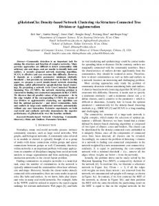
in viral marketing and epidemiology could be central nodes for spreading ideas or diseases. On the contrary, outliers are marginally connected with the community members. Since the characteristics of outliers deviate significantly from the communities, they should be isolated as noise. Therefore, how to detect communities as well as hubs and outliers in a network becomes an interesting and challenging problem. Most existing approaches only study the problem of community detection without considering hubs and outliers. A density-based network clustering algorithm SCAN [2] can overcome this difficulty. However, it needs user to specify a minimum similarity 𝜀 and a minimum cluster size 𝜇 to define clusters, and is sensitive to the parameter 𝜀 which is difficult to determine. Actually, how to locate the optimal parameter 𝜀 automatically for the density-based clustering methods (e.g., DBSCAN [3] and SCAN) is a long-standing and challenging task. The connectivity structure of a large-scale network is highly complex, which makes the selection of optimal parameter 𝜀 difficult. However, we have found that a cluster defined by density-based clustering algorithms is composed of two types of objects: cores and borders. The cluster can be determined by the density-connected cores embedded in it uniquely. Hence, once all the components of connected cores have been detected, all clusters can be revealed. Accordingly, we convert the problem of detecting 𝜀-clusters in a network to finding core-connected components in the network weighted by a new measurement: core-connectivitysimilarity. It is equal to partitioning the core-connected network with a minimal threshold 𝜀 (i.e., remove all the edges whose weights are below 𝜀 from the network). Actually, the problem above can be easily solved by the Maximal Spanning Tree (MST), a connectivity skeleton of the network [4]. To motivate this, we illustrate a schematic network in Figure 1(a). Given 𝜀 = 3, if all the edges with weights no more than current 𝜀 are removed from the network, two unconnected sub-graphs will emerge, as shown in Figure 1(c). In contrast, if we first construct the MST of the network, as shown in Figure 1(b), and then partition the MST with the same threshold, the partitioning result on the MST is equal to that on the original network. In the
3
5 2 1
3
5 4
4
4
2
4
4
4
5 4
3
3
5 6
3
5 1
4
5
8 3
5
2
5 1 4
2
5 4
5
5 4
9
4
4
8
3
6
(c)
II. R ELATED WORK
5
Equivalent
1 4
7
4
9
4
4
5
section 5, we describe the algorithms in detail. In section 6, we report the experimental results. Finally, we summarize our conclusions and suggest future work in section 7.
Partition
4 4
7
(b) Partition
4
4
6
(a)
3
9 5
5
4 7
3
4 4
MST 4
8
3
1
9 5
2
2
5
5
5
8 4
5 6
7
(d)
Figure 1. A schematic network: (a) the original network, (b) the MST of the network, (c) the partition of the original network with 𝜀 = 3, (d) the partition of the MST with 𝜀 = 3.
same way, the core-connected components can be detected on the Core-Connected Maximal Spanning Tree (CCMST) of the network. Since each edge of the CCMST is a cut edge, different edge weights will lead to different partition results and form different clusters. It also means that all possible 𝜀, which we can adopt to cluster the network, can be found in the edge weights of the CCMST. Furthermore, the best clustering result can be selected by a quality function. In this paper, a novel density-based network clustering algorithm, called gSkeletonClu, is proposed to perform the clustering on the CCMST. To our best knowledge, our work is the first that builds the connection between the densitybased clustering principle and the MST-based clustering method. The main contributions of this paper are summarized in the following: 1) By projecting the network to its CCMST, we convert the community discovery problem to finding coreconnected components in the CCMST. Consequently, we only need to deal with the essential edges of the network which reduces the size of the candidate solution space significantly. We have proven that the clustering result on the CCMST is equal to that on the original network. 2) We discover that all possible values of the parameter 𝜀 lie in the edge weights of the corresponding CCMST. Using the modularity measure 𝑄𝑠 , our algorithm can select the optimal parameter 𝜀 automatically, without any user interaction. 3) Our algorithm not only uncovers the communities within the network, but also identifies the hubs and outliers. Experimental results show that our algorithm is scalable and achieves high accuracy. 4) Our algorithm can overcome the chaining effect that the traditional MST clustering methods suffer from and the resolution limit possessed by other modularitybased algorithms. The rest of the paper is organized as follows. First we briefly review the related work in Section 2. In section 3, we introduce the concepts of structural-connected clusters. In section 4, we formulize the notion of clusters derived from the CCMST and present the theoretical analysis. In
The problem of detecting communities within networks has been extensively studied for years. Graph partitioning is a natural choice for this problem, such as Kernighan-Lin algorithm [5], Metis [6], and normalized cut [7]. To make the calculation of cut functions more efficient, spectral clustering method has been proposed where the eigenvectors of certain normalized similarity matrices are used for the clustering purpose [8]. Since the community structure in networks is highly complex, new clustering methods have recently been introduced to solve this challenging problem. Density-based Clustering Methods: Density-based clustering approaches (e.g., DBSCAN [3] and OPTICS [9]) have been widely used in data mining owing to their ability of finding clusters of arbitrary shape even in the presence of noise. Recently, Xu et al. proposed a structural network clustering algorithm SCAN [2] extended from DBSCAN. This algorithm can find communities as well as hubs and outliers. However, the main difficulty for the SCAN algorithm is that it is sensitive to the minimal threshold 𝜀 of the structuresimilarity. A simple “knee hypothesis” has been presented to locate the parameter 𝜀 manually for the SCAN algorithm. However, the knee dose not always correspond to the optimal 𝜀 value. More importantly, there are no obvious knees on the k-nearest ranked similarity plot for most of the real-world networks. To deal with this problem, Bortner et al. proposed a new algorithm, called SCOT+HintClus [10], to detect the hierarchical cluster boundaries of network through extension of the algorithm OPTICS [9]. However, it does not find the global optimal 𝜀. Our work tries to solve the sensitive parameter problem of density-based network clustering from another angle. Graph-theoretical Clustering Methods: Clustering algorithms based on graph theory can be used to detect clusters of different shapes and sizes. One of the best-known graph-based hierarchical clustering algorithms is based on the construction of the minimal (or maximal) spanning tree (MST) of the objects which was initially proposed by Zahn [11]. The standard MST divisive algorithm removes edges from the MST in order of decreasing length until the specified number of clusters results. A clustering algorithm using an MST takes the advantage that it is able to only consider the necessary connections between the data patterns and the cost of clustering can be decreased. However, the number of the desired clusters should be given in advance. Moreover, simple linkage-based methods often suffer from the problem of chaining effect. Some clustering algorithms have been shown closely related to MST, such as Singlelink [12]. Recently, some researchers utilized the MSTbased clustering method to analyze complex networks [13].
s
Definition 1. (Structural Similarity) Let 𝐺 = (𝑉, 𝐸, 𝑤) be a weighted undirected network and 𝑤(𝑒) be the weight of the edge 𝑒. For a node 𝑢 ∈ 𝑉 , we define 𝑤({𝑢, 𝑢}) = 1. The structure neighborhood of a node 𝑢 is the set Γ(𝑢) containing 𝑢 and its adjacent nodes which are incident a common edge with 𝑢 : Γ(𝑢) = {𝑣 ∈ 𝑉 ∣{𝑢, 𝑣} ∈ 𝐸} ∪ {𝑢}. The structural similarity between two adjacent nodes 𝑢 and 𝑣 is then ∑ 𝑤(𝑢, 𝑥) ⋅ 𝑤(𝑣, 𝑥) 𝑥∈Γ(𝑢)∩Γ(𝑣)
𝜎(𝑢, 𝑣) = √ ∑
𝑥∈Γ(𝑢)
𝑤2 (𝑢, 𝑥) ⋅
√ ∑ 𝑥∈Γ(𝑣)
𝑤2 (𝑣, 𝑥)
.
(1)
p
0.8
Given a minimum similarity 𝜀 and a minimum cluster size 𝜇, the main idea of structure-connected clustering is that for each node in a cluster, it must have at least 𝜇 neighbors whose structural similarities are at least 𝜀. In this section, we formulize the notion of a structure-connected cluster, which extends that of a density-based cluster [3], [9].
0.87 0 .7
0.8
q
2 0.8 r
0.75
t
0.8
III. P RELIMINARIES
0.75
Our work introduces tree clustering into the framework of density-based clustering which is rather different from the traditional MST-based clustering method. Quality Functions for Network Clustering: Clustering validity checking is an important issue in cluster analysis [14]. For community detection, the most popular quality function is the modularity measure 𝑄 proposed by Newman and Girvan [15]. Recently, a similarity-based modularity function 𝑄𝑠 was presented by Feng et al. [16] through extension from the connection-based modularity 𝑄, which has a better ability to deal with hubs and outliers. The 𝑄𝑠 function is defined as follows: [ ( )2 ] 𝑘 ∑ 𝐷𝑆𝑖 𝐼𝑆𝑖 − 𝑄𝑠 = , 𝑇𝑆 𝑇𝑆 𝑖=1 ∑ where 𝑘 is the number of clusters, 𝐼𝑆𝑖 = 𝑢,𝑣∈𝐶𝑖 𝜎(𝑢, 𝑣) is the total similarity of nodes within cluster 𝐶𝑖 , 𝐷𝑆𝑖 = ∑ 𝑢∈𝐶𝑖 ,𝑣∈𝑉 𝜎(𝑢, 𝑣) is the total similarity between nodes in ∑ cluster 𝐶𝑖 and any node in the network, and 𝑇 𝑆 = 𝑢,𝑣∈𝑉 𝜎(𝑢, 𝑣) is the total similarity between any two nodes in the network. Modularity optimization itself is a popular method for community detection. Most modularity-based algorithms find the optimal clustering result via greedily maximizing the value of 𝑄, such as FastModularity [17] and Simulated Annealing (SA for short) [18]. However, recent research shows that modularity is not a scale-invariant measure, and hence, by relying on its maximization, detection of communities smaller than a certain size is impossible. This serious problem is well known as the resolution limit [19]. Compared with the traditional modularity-based methods, our work uses modularity as a quality function to guide the selection of optimal clustering results.
Figure 2. The structure reachablility and structure connectivity relationship of the nodes in a density-based cluster.
The above structural similarity is extended from a cosine similarity used in [2] which denotes the local connectivity density of any two adjacent nodes in an undirected network. It can be replaced by other similarity definitions such as Jaccard similarity, and our experimental results show that the cosine similarity is better. Definition 2. (Core) For a node 𝑢, the set of neighbors having structural similarity greater than 𝜀 forms the 𝜀neighborhood of 𝑢: (2) Γ𝜀 (𝑢) = {𝑣 ∈ Γ(𝑢)∣𝜎(𝑢, 𝑣) ≥ 𝜀}. If ∣Γ𝜀 (𝑢)∣ ≥ 𝜇, then 𝑢 is a core node, denoted by K𝜀,𝜇 (𝑢). A core node is the one whose 𝜀-neighborhood is at least 𝜇. As shown in Figure 2, when we set 𝜀 = 0.75 and 𝜇 = 4, node 𝑝 is a core and node 𝑞 is in the 𝜀-neighborhood of 𝑝. According to the principle of density-based clustering, the clusters grow from core nodes. If a node is in the 𝜀neighborhood of a core, it should be in the same cluster with the core. This idea is formulized in the following definition of direct structure reachability. Definition 3. (Structure-Reachable) Given 𝜀 ∈ ℝ, 𝜇 ∈ ℕ, a node 𝑣 ∈ 𝑉 is directly structure-reachable from a node 𝑢 ∈ 𝑉 iff K𝜀,𝜇 (𝑢)∧𝑣 ∈ Γ𝜀 (𝑢), denoted by 𝑢 →𝜀,𝜇 𝑣. A node 𝑣 ∈ 𝑉 is structure-reachable from 𝑢 ∈ 𝑉 iff ∃{𝑢1 , ..., 𝑢𝑛 } ⊆ 𝑉 s.t. 𝑢 = 𝑢1 , 𝑣 = 𝑢𝑛 , and ∀𝑖 ∈ {1, 2, ..., 𝑛 − 1} such that 𝑢𝑖 →𝜀,𝜇 𝑢𝑖+1 . This is denoted by 𝑢 →𝜀,𝜇 𝑣. A node 𝑣 ∈ 𝑉 is directly structure-reachable from a core node 𝑢 ∈ 𝑉 if 𝑣 ∈ Γ𝜀 (𝑢). Obviously, directly structurereachable is symmetric for pairs of core nodes. If a non-core node 𝑣 is directly structure-reachable from a core node 𝑢, then 𝑣 is a border node attached to 𝑢. In general, directly structure-reachable is not symmetric if a core node and a border node are involved. We depict the notion of structure-reachable in Figure 2. When we set 𝜀 = 0.75 and 𝜇 = 4, there are four nodes in the neighborhood of node 𝑝, 𝑞 and 𝑟 respectively, whose structure similarities with them are greater than current 𝜀, thus 𝑝, 𝑞 and 𝑟 are all core nodes. Since the structure similarity between 𝑝 and 𝑞 is greater than 0.75, 𝑝 and 𝑞 are directly structure-reachable from each other. And for the same reason, 𝑟 and 𝑞 are also directly structure-reachable from each other. According to Definition 3, core nodes 𝑝, 𝑞 and 𝑟 are structure-reachable from each other. However, the border node 𝑠 is only structure-reachable from the three core nodes on one side. The transitive closure of directly structure-reachable relation forms clusters, and any pair of nodes in the same cluster is structure connected.
Cluster 1 Cluster 2 Figure 3. An example network with two structure-connected clusters, one hub and two outliers.
The core-similarity of a node 𝑢 is the maximum of structural-similarity 𝜀˜ such that 𝑢 would be a core node w.r.t. ∣Γ𝜀˜(𝑢)∣ ≥ 𝜇. Otherwise, the core-similarity is zero. As shown in Figure 4(a), the core-similarity of node 𝑝 is 0.75 when 𝜇 = 4, because the size of the 𝜀-Neighborhood of node 𝑝 is just four when 𝜀 = 0.75 and node 𝑝 will no longer be a core when 𝜀 > 0.75.
Definition 4. (Structure-Connected Cluster) The set 𝐶[𝑢] ⊆ 𝑉 is a cluster represented by K𝜀,𝜇 (𝑢) ∈ 𝑉 iff (1)𝑢 ∈ 𝐶[𝑢]; (2)∀𝑣 ∈ 𝑉 , 𝑢 →𝜀,𝜇 𝑣 ⇒ 𝑣 ∈ 𝐶[𝑢]; and (3)∣𝐶[𝑢]∣ ≥ 𝜇.
Definition 7. (Reachability-Similarity) Given 𝑢, 𝑣 ∈ 𝑉 , the reachability-similarity of 𝑣 w.r.t. 𝑢 is 𝑅𝑆(𝑢, 𝑣) ≡ min{𝐶𝑆(𝑢), 𝜎(𝑢, 𝑣)}.
A cluster 𝐶 contains exactly the nodes which are structure-reachable from an arbitrary core in 𝐶. If there are two core nodes 𝑢, 𝑣 ∈ 𝑉 s.t. 𝑢 →𝜀,𝜇 𝑣, then 𝐶[𝑢] = 𝐶[𝑣]. Consequently, a cluster is uniquely determined by the connected core nodes in it. As shown in Figure 3, cluster 1 contains all the nodes which are structure-reachable from core nodes 𝑝, 𝑞 and 𝑟. Thus, 𝐶[𝑝] = 𝐶[𝑞] = 𝐶[𝑟]. There also may exist some border nodes (e.g., node 𝑠 in Figure 3). Given parameters 𝜀 and 𝜇, a clustering of a network 𝐺 is the set 𝐶𝑅𝜀,𝜇 of distinct structure-connected clusters found in the network. After the network is clustered, there are still some nodes that are not suitable to be assigned to any cluster and they may be hubs or outliers.
Intuitively, the reachability-similarity of a node 𝑣 w.r.t. a core node 𝑢 is the maximum of structural similarities such that 𝑣 is directly structure-reachable from 𝑢. As shown in Figure 4(a), the reachability-similarity of node 𝑞 w.r.t. core node 𝑝 is 0.75 which is equal to the core-similarity of node 𝑝, because the similarity between the two nodes is not less than the core-similarity of 𝑝. While the reachability-similarity of node 𝑟 w.r.t. core node 𝑝 is 0.7 which is equal to the similarity between 𝑝 and 𝑟.
s p
q
r
o2
h
o1
Definition 5. (Hub and Outlier) Given parameters 𝜀, 𝜇, and a clustering 𝐶𝑅𝜀,𝜇 of the network 𝐺, a node ℎ ∈ 𝑉 is a hub iff (1) ℎ does not belong to any cluster: ∀𝐶[𝑢] ∈ 𝐶𝑅𝜀,𝜇 , ℎ∈ / 𝐶[𝑢]; (2) ℎ bridges multiple clusters: ∃𝐶, 𝐷 ∈ 𝐶𝑅𝜀,𝜇 , 𝐶 ∕= 𝐷, 𝑢 ∈ 𝐶 ∧ 𝑣 ∈ 𝐷, 𝑠.𝑡. ℎ ∈ Γ(𝑢) ∧ ℎ ∈ Γ(𝑣). Any node that is not in a cluster and not a hub is called an outlier. As shown in Figure 3, node ℎ that connects two nodes of different clusters is regarded as a hub, and nodes 𝑜1 and 𝑜2 , which are connected with only one cluster, should be regarded as outliers. IV. CLUSTERS DERIVED FROM CORE-CONNECTED MST To introduce the notion of core-derived clusters, we make the following observation: each cluster is determined by the structure-connected core nodes in it. Given {𝑢, 𝑣} ∈ 𝐸, we must decide whether 𝑢 and 𝑣 are core nodes w.r.t. current 𝜀 and whether 𝑢 and 𝑣 are structure-reachable from each other. If so, 𝑢 and 𝑣 will lie in the same cluster. Our new algorithm gSkeletonClu bases on the principle of finding the core-connected components at different 𝜀 levels. The involved concepts are introduced in the following. A. Core Connectivity Similarity Definition 6. (Core-Similarity) Given a node 𝑢 ∈ 𝑉 , the core-similarity of 𝑢 is ⎧ ⎨ max{𝜀 ∈ ℝ+ : 𝐶𝑆(𝑢) ≡ ∣{𝑣 ∈ Γ(𝑢) : 𝜎(𝑢, 𝑣) ≥ 𝜀}∣ ≥ 𝜇} ⎩ 0
∣Γ(𝑢)∣ ≥ 𝜇 𝑜𝑡ℎ𝑒𝑟𝑤𝑖𝑠𝑒.
(3)
(4)
Definition 8. (Core-Connected) Given 𝜀 ∈ ℝ, 𝜇 ∈ ℕ, 𝑢, 𝑣 ∈ 𝑉 , 𝑢 and 𝑣 are directly core-connected with each other iff K𝜀,𝜇 (𝑢) ∧ K𝜀,𝜇 (𝑣) ∧ 𝑢 →𝜀,𝜇 𝑣. This is denoted by 𝑢 ↔𝜀,𝜇 𝑣. Since directly structure-reachable is symmetric for any pair of core nodes, if two core nodes are directly structurereachable from each other, then they are directly coreconnected. The transitive closure of the directly coreconnected relation forms core-connected components, and any pair of nodes in the same component are core-connected. Definition 9. (Core-Connectivity-Similarity) Given {𝑢, 𝑣} ∈ 𝐸, the core-connectivity-similarity of 𝑢 and 𝑣 is 𝐶𝐶𝑆(𝑢, 𝑣) ≡ min{𝑅𝑆(𝑢, 𝑣), 𝑅𝑆(𝑣, 𝑢)} . ≡ min{𝐶𝑆(𝑢), 𝐶𝑆(𝑣), 𝜎(𝑢, 𝑣)}
(5)
The core-connectivity-similarity of two nodes is the minimum of their core-similarities and the structure-similarity between them. As shown in Figure 4(a), nodes 𝑝 and 𝑞 are core-connected when 𝜀 = 0.75 and 𝜇 = 4, because 𝑝 and 𝑞 are both core nodes and their structure-similarity is not less than the current 𝜀. But if we set current 𝜀 > 0.75, nodes 𝑝 and 𝑞 are not core-connected any more, because 𝑝 will not be a core under this configuration. Thus, the core-connectivitysimilarity of 𝑝 and 𝑞 is 0.75 when 𝜇 = 4. The following Theorem 1 shows that the core-connectivity-similarity of two nodes is the maximal structural similarity such that they are both core nodes and directly core-connected from each other. Theorem 1. Given a network 𝐺 = (𝑉, 𝐸, 𝑤), {𝑢, 𝑣} ∈ 𝐸, 𝜇 ∈ ℕ, if 𝐶𝐶𝑆(𝑢, 𝑣) = 𝜀ˆ, then 𝜀ˆ is the maximum of 𝜀 s.t. 𝑢 ↔𝜀,𝜇 𝑣. For each edge 𝑒 = {𝑢, 𝑣} ∈ 𝐸 in a weighted network 𝐺 = (𝑉, 𝐸, 𝑤), we calculate the core-connectivitysimilarity for each pair of adjacent nodes 𝑢 and 𝑣. Set 𝜛(𝑒) = 𝐶𝐶𝑆(𝑢, 𝑣). Then we get a core-connected network
Definition 10. (Connectivity Level) Let 𝐺 = (𝑉, 𝐸, 𝜛) be a core-connected undirected network and each edge 𝑒 ∈ 𝐸 has a value of core-connectivity-similarity 𝜛(𝑒) ∈ [0, 1]. Given nodes 𝑢, 𝑣 ∈ 𝑉 , 𝑢 ∕= 𝑣 and 𝜀 ∈ ℝ, 𝑢 and 𝑣 are connected if each edge 𝑒 ∈ 𝐸 𝑠.𝑡. 𝜛(𝑒) < 𝜀 is removed from 𝐺, but they are not connected if each edge 𝑒 ∈ 𝐸 𝑠.𝑡. 𝜛(𝑒) ≤ 𝜀 is removed from 𝐺. Then the connectivity level of 𝑢 and 𝑣 in 𝐺 is 𝜀. This is denoted by 𝛾𝐺 (𝑢, 𝑣) = 𝜀. Theorem 2. Let 𝐺 = (𝑉, 𝐸, 𝜛) be a core-connected undirected network and 𝑇 be an MST of 𝐺. ∀𝑢, 𝑣 ∈ 𝑉, 𝑢 ∕= 𝑣, 𝛾𝐺 (𝑢, 𝑣) = 𝛾𝑇 (𝑢, 𝑣). Proof: ∀𝑢, 𝑣 ∈ 𝑉 , 𝑢 ∕= 𝑣, let 𝛾𝑇 (𝑢, 𝑣) = 𝜀, and 𝑃 be the path between 𝑢 and 𝑣 in 𝑇 . Obviously, ∃𝑒 = {𝑝, 𝑞} ∈ 𝑃 𝑠.𝑡. 𝜛(𝑒) = 𝜀 and 𝜀 is the minimal edge weight in 𝑃 . When each edge 𝑑 s.t. 𝜛(𝑑) < 𝜀 is removed from 𝐺, path 𝑃 still remains in 𝐺. Thus, nodes 𝑢 and 𝑣 will stay connected in 𝐺. Assume that each edge 𝑑 ∈ 𝐸 s.t. 𝜛(𝑑) ≤ 𝜀 is removed from 𝐺, 𝑢 and 𝑣 are still connected. There must be a path 𝑃 ′ between 𝑢 and 𝑣 in 𝐺 s.t. ∀𝑑 ∈ 𝑃 ′ , 𝜛(𝑑) > 𝜀. So / 𝑇 , otherwise 𝑃 and 𝑃 ′ will form ∃𝑒′ = {𝑝′ , 𝑞 ′ } ∈ 𝑃 ′ ∧ 𝑒′ ∈ ′ a cycle in 𝑇 . 𝑇 = (𝑇 − {𝑒}) ∪ {𝑒′ } is also a Spanning Tree of 𝐺 s.t. 𝜛(𝑇 ′ ) > 𝜛(𝑇 ). It is inconsistent with that 𝑇 is a maximal spanning tree of 𝐺. So 𝑢 and 𝑣 will not be connected when each edge 𝑑 ∈ 𝐸 s.t. 𝜛(𝑑) ≤ 𝜀 is removed from 𝐺. Thus 𝛾𝐺 (𝑢, 𝑣) = 𝛾𝑇 (𝑢, 𝑣) = 𝜀. Since each edge of 𝑇 is a cut edge, different edge weights of 𝑇 will produce different partition results and form different clusters. Without considering the slight effect of border nodes, all possible 𝜀 values lie in the edge weights of the CCMST.
03
3
5 0 .7
6
0.7 5
0.7303
303
0.7 3
0.730 3
0.7
0
2
8 70 0.6
1
11
Phase 1. Construct CCMST 4 3 7303 12
13 0. 14
7
5
10
3 0.730 0.7 30 3
6
0.7
5
2
1
11
Ω Candidates μ=3
3
5 0.7
0.7 30
9
0.730 3
8
Phase 2.1 Detect core-connected components with Ω=0.7303 4
Ω=0.7303 μ=3
3 30 0.7
14 Outlier
10
0.7
0.7 3 Borders 03
303
8 9
7303 12
13 0.
03 0.73
According to the Cut Property of MST, we can prove that partitioning core-connected network 𝐺 with 𝜀 (remove edge 𝑒 s.t. 𝜛(𝑒) ≤ 𝜀 from 𝐺) is equal to the partition of its CCMST with 𝜀.
0.5
3 0.730 5 0 0.5 .73 071 03
0.6761
71
03
B. Partition Networks on Its CCMST
0.6
7
0.6708
4
0.73
𝐺 = (𝑉, 𝐸, 𝜛). Note that the core-connectivity-similarity of any two adjacent nodes is equal to their structure similarity when 𝜇 = 2, because here the core-similarity of two adjacent nodes is equal to the highest similarity of their incident edges which is not less than their structure-similarity. Hence, the CCMST of a core-connected network is equal to the MST of the original network when 𝜇 = 2.
0.75 0.7303 0.6761 0.6708 0
10
7303 12 0.6761
13 0.
0.730 3
0.65
0.6 8
0.8
(a) (b) Figure 4. (a)an example for calculating core-similarity and reachabilitysimilarity; (b)an example for calculating attachability-similarity and finding attractor.
Ω Candidates μ=3
0.0
8 70 0.6
03 0.73
0.7
8 0.6
r
14
0.6708
0.8
attractor
p
071
1
0.75
0.82
0.75
07 0. 5
303 0.7
0.8
9
0.5
03 73
q
q
8
708 0.6 0.6 708
0.
0 .8
p 0.75 0.82
0.75 0.7303 0.6761 0.6708 0
11 Cluster 1
7 Hub
5
5 0 .7
3 0.730 0 .7 30 3
6
0. 7 5
3
2
1 Cluster 2
Phase 2.2 Attach borders and form clusters Figure 5.
Procedure of the network clustering on the CCMST.
C. Bulid the Attractor Indices The partition on the CCMST of a network can detect the core nodes for each cluster. In addition, there may exist some border nodes in a cluster. In order to attach the border nodes of each cluster efficiently, we build the indices in advance. The involved concepts are given as follows. Definition 11. (Attachability-Similarity) Given 𝑣 ∈ 𝑉 , the attachability-similarity of 𝑣 w.r.t. its neighbor nodes is 𝐴𝑆(𝑣) = max{𝑅𝑆(𝑢, 𝑣)∣𝑢 ∈ Γ(𝑣) − {𝑣}}.
(6)
The attachability-similarity of a node 𝑣 is the maximum of reachability-similaries w.r.t. its neighbor nodes. The neighbor node that possesses the maximal reachability-similarity to 𝑣 is regarded as the attractor of 𝑣. If 𝐶𝑆(𝑣) < 𝐴𝑆(𝑣) (i.e., the core-similarity of 𝑣 is less than its attachability-similarity), then 𝑣 is not a core node, but its attractor 𝑢 is a core node when 𝜀 = 𝐴𝑆(𝑣). That is to say, 𝑣 should be attached as a border node to the cluster containing core node 𝑢. In this case, an index of the attachability-similarity for node 𝑣 and its attractor 𝑢 will be built in advance. As shown in Figure 4(b), the reachabilitysimilarities of node 𝑝 w.r.t. its neighbor nodes are labeled on the arrowhead lines. Since the value of reachabilitysimilarity from 𝑞 to 𝑝 is the highest, node 𝑞 should be the attractor of 𝑝 and the attachability-similarity of node 𝑝 is 0.82 which is equal to the reachability-similarity of 𝑝 w.r.t 𝑞. Note that the attractor can be selected arbitrarily with ties and the indices can be built during the calculation of core-connectivity-similarity.
V. THE ALGORITHM Our network clustering algorithm on the CCMST includes two phases, and the procedure is illustrated in Figure 5. In the first phase, we calculate the core-connectivity-similarity for each edge in the network, build the attractor indices and construct the CCMST accordingly. After that, we record all the different edge weights of the CCMST as the 𝜀 candidates and sort them ascending or descending. In the second phase, we perform the tree clustering on the CCMST. Actually, the clustering results are not sensitive to the parameter 𝜇 which can be set as a constant. There are two different ways to implement the tree clustering. The first is tree agglomerative clustering and the pseudocode is given in Algorithm 1. We consider an initial forest consisting of 𝑛 isolated nodes. Then we add the edges having the same weights in the CCMST to the forest, from the highest value to the lowest. For each 𝜀, it will agglomerate the nodes into multiple core-connected components after all the edges whose weights are equal to 𝜀 have been added to the forest. After attaching the border nodes, we can get the clusters. Then we calculate the 𝑄𝑠 value of current clustering result. The output of the algorithm is the clusters with the highest 𝑄𝑠 value and the corresponding 𝜀. The second method is tree divisive clustering. We remove the edges in the CCMST w.r.t. different weights or 𝜀, from the lowest value to the highest. For each 𝜀, it will partition the tree into multiple core-connected components. The remaining process is the same as the agglomerative one. The two tree clustering algorithms above are equivalent in clustering results, but the agglomerative one is convenient for detecting the connected components in the forest. Thus, it is faster than the divisive one. Because the core-connectivitysimilarity of any two nodes is equal to their structuresimilarity when 𝜇 = 2, the procedure of attaching borders can be passed over in this case. Hence, our algorithm contains the traditional MST-based clustering as a special case. We also compared our algorithm with the SCAN algorithm. Though the clustering procedures of gSkeletonClu and SCAN are quite different, the results of these two algorithms are almost the same w.r.t. the same values of parameters 𝜀 and 𝜇. In addition, our algorithm can detect overlapping communities by permitting hubs and border nodes to be shared by multiple clusters. The running time of gSkeletonClu is mainly consumed by the construction of CCMST and tree clustering. The core-connectivity-similarity and attractor indices can be calculated within a complexity of 𝑂(𝑚). We construct the CCMST of the core-connected network using the Prim’s algorithm with a Fibonacci Heap. Its running time complexity is 𝑂(𝑚 log 𝑛). In the procedure of agglomerative clustering, we only need to add the edges to the forest in order of weights with a complexity of 𝑂(𝑛 log 𝑛). However, the calculation of 𝑄𝑠 is a little time consuming. We implement
Algorithm 1 gSkeletonClu Agglomerative Input: Network 𝐺 = (𝑉, 𝐸, 𝑤); and 𝜇 ∈ ℕ Output: Clusters 𝐶𝑅 = {𝐶1 , 𝐶2 , ⋅ ⋅ ⋅ , 𝐶𝑚 }; hubs and outliers N; and optimal 𝜀 1: //Phase 1: Construct CCMST 𝑇 = (𝑉, 𝐸 ′ ) 2: Initialize a empty dynamical priority queue 𝐴𝐼𝑄; 3: for each 𝑒 = {𝑢, 𝑣} ∈ 𝐸 do 4: CalculateCCS(𝑢, 𝑣, 𝜇); 5: BuildAttractorIndices(𝐴𝐼𝑄, 𝑢, 𝑣); 6: end for 7: 𝑇 = 𝑀 𝑆𝑇 (𝐺); 8: 𝑊 = {𝐶𝐶𝑆(𝑒)∣𝑒 ∈ 𝐸 ′ }; 9: 𝑆𝑜𝑟𝑡 𝐷𝑒𝑐𝑒𝑛𝑑(𝑊 ); 10: //Phase 2: Tree Clustering 11: 𝐸 (0) = ∅; 12: 𝐹 (0) = (𝑉, 𝐸 (0) ); 13: for 𝑖 = 1 𝑡𝑜 ∣𝑊 ∣ do 14: //Phase 2.1: Detect connected components 15: 𝜀(𝑖) = 𝑊 [𝑖]; 16: 𝑆 = {{𝑣𝑖 , 𝑣𝑗 }∣{𝑣𝑖 , 𝑣𝑗 } ∈ 𝐸 ′ ∧ 𝐶𝐶𝑆(𝑣𝑖 , 𝑣𝑗 ) = 𝜀(𝑖) }; 17: 𝐸 (𝑖) = 𝐸 (𝑖−1) ∪ 𝑆; 18: 𝐹 (𝑖) = (𝑉, 𝐸 (𝑖) ); 19: 𝐶𝑅(𝑖) = {𝐶[𝑐]∣𝑐 ∈ 𝑉 , 𝐶[𝑐] is a connected component in 𝐹 (𝑖) }; 20: //Phase 2.2: Attach borders 21: while 𝐴𝐼𝑄.getHead().KeyValue ≥ 𝜀(𝑖) do 22: (𝑝, 𝑞, 𝐾𝑒𝑦𝑉 𝑎𝑙𝑢𝑒) = 𝐴𝐼𝑄.popHead(); 23: if {{𝑝}} ∈ 𝐶𝑅 then 24: 𝐶[𝑞] = 𝐶[𝑞] ∪ {𝑝}; 25: 𝐶𝑅 = 𝐶𝑅 − {{𝑝}}; 26: end if 27: end while 28: //Phase 2.3: Detect clusters, hubs and outliers 29: 𝑁 (𝑖) = ∅; 30: for each C ∈ 𝐶𝑅(𝑖) do 31: if ∣𝐶∣ < 𝜇 then 32: 𝐶𝑅(𝑖) = 𝐶𝑅(𝑖) − {𝐶}; 33: 𝑁 (𝑖) = 𝑁 (𝑖) ∪ 𝐶; 34: end if 35: end for 36: 𝑄(𝑖) = 𝑄𝑠 (𝐶𝑅(𝑖) ); 37: end for 38: 𝑘 = arg max𝑡 {𝑄(𝑡) }; 39: return 𝐶𝑅(𝑘) , 𝑁 (𝑘) and 𝜀(𝑘) ;
it in an incremental way and the complexity is 𝑂(𝑚) when we try all possible 𝜀. In total, the time complexity of our algorithm is 𝑂((𝑚+𝑛) log 𝑛). For the scale-free networks, it is 𝑂(𝑚 log 𝑛). The algorithm can also be implemented in a more efficient way, which starts the clustering process from the 1/2 of ordered edges and stops when the current 𝑄𝑠 value decreases by 0.05 from the previous one. The optimized algorithm reduces almost 1/2 running time with the same clustering results. VI. EXPERIMENTS In this section, we evaluate the proposed algorithm using some real-world networks and synthetic datasets. The performance of gSkeletonClu is compared with two state-of-the-art methods: SCAN and FastModularity. SCAN is an efficient density-based network clustering algorithm, and FastModularity is a representative modularity-based algorithm for community detection. Our algorithm is implemented using
Table I T HE PARAMETERS OF THE COMPUTER - GENERATED DATASETS FOR PERFORMANCE EVALUATION . 𝑛 10,000 10,000 100,000 100,000
𝑚 99,238 99,036 1,987,850 1,990,271
𝑘 20 20 40 40
𝑚𝑎𝑥𝑘 50 50 100 100
𝑚𝑖𝑛𝑐 10 20 50 100
𝑚𝑎𝑥𝑐 50 100 100 200
ANSI C++. All the experiments were conducted on a PC with a 2.4 GHz Pentium IV processor and 4GB of RAM. A. Datasets We evaluate the performance of our algorithm on two types of datasets. One is the real-world networks and the other is the computer-generated benchmark networks with known community structure. 1) Real-world Networks: To assess the performance of the proposed method in terms of accuracy, we conduct experiments on two popular real-world networks: NCAA College-football network and US Political Books network [20]. The NCAA College-football is a social network with communities (or conferences) of American college football teams. The network, representing the schedule of Division I-A games for the 2000 season, contains 115 nodes and 613 edges. All college football teams are divided into eleven conferences and five independent teams (Utah State, Navy, Notre Dame, Connecticut and Central Florida) that do not belong to any conference. There is a link between two teams if they played a game together. Now the question is to find out the communities from the graph that represents the schedule of games played by all teams. The network of US Political Books contains 105 nodes and 441 edges. The nodes of the network represent the US political books sold by the online bookseller Amazon.com and have been given labels “liberal”, “neutral”, or “conservative”, respectively, by Newman. There is a link between two books if they are copurchased frequently enough by the same buyers. 2) Synthetic Benchmark Networks: We also use the Lancichinetti-Fortunato-Radicchi (LFR) benchmark graphs [21] to evaluate the performance of our algorithm. By varying the parameters of the networks, we analyze the behavior of the algorithms in detail. Some important parameters of the benchmark networks are: ∙ 𝑛: number of nodes ∙ 𝑚: average number of edges ∙ 𝑘: average degree of the nodes
𝑚𝑎𝑥𝑘: maximum degree 𝑚𝑢: mixing parameter, i.e., each node shares a fraction of its edges with nodes in other communities 𝑚𝑖𝑛𝑐: minimum for the community sizes 𝑚𝑎𝑥𝑐: maximum for the community sizes
We generate several weighted undirected benchmark networks with the number of nodes 𝑛 = 10,000 and 100,000. In Table I, we list the values of the parameters for the generated datasets. For each 𝑛, two types of networks are generated with different ranges of the community sizes, where S means that the sizes of the communities in the dataset are relatively small and B means that the sizes of the communities are relatively big. For each type of datasets, we generate fifteen networks with different mixing parameter 𝑚𝑢 ranging from 0.1 to 0.8 with a span of 0.05. Generally, the higher the mixture parameter of a network is, the more difficult it is to reveal the community structure. B. Selection of the Parameter 𝜀 In [2], the authors presented a “knee hypothesis” to find the proper 𝜀 value. We sort 3-nearest similarity of all nodes in the networks to locate the knee. Two plots for the US Political Books and the benchmark 10000B are given respectively in Figure 6, and it can be observed that there are no obvious knee in the curves. Furthermore, there is no rigorous way to ensure that the identified “knees” are the appropriate values of the parameter 𝜀. In the experiment, we try our best to select a “knee” as the parameter 𝜀 for the SCAN algorithm from the 3-nearest similarity plot of each network. In contrast, our algorithm locate the optimal 𝜀 automatically which achieves the highest 𝑄𝑠 value. In Table II, we show the manually selected values of 𝜀 and the corresponding 𝑄𝑠 for some adopted datasets, as well as the optimal 𝜀 and the corresponding 𝑄𝑠 values found by gSkeletonClu, where 𝑚𝑢 = 0.4 for all of the benchmark networks. As shown in Table II, the manually selected 𝜀 is NCAA College−football
0.6
0.8
0.5
0.6
US Political Books 0.6 0.5 0.4
0.4
Qs
3−nearest similarity
3−nearest similarity
0.8
35 70 Rank of nodes
football polbooks 10000S 10000B 100000S 100000B
10000B (mu=0.4)
US Political Books 0.9
0.2 0
Dataset
Qs
Dataset 10000S 10000B 100000S 100000B
Table II T HE OPTIMAL 𝜀 AND THE CORRESPONDING 𝑄𝑠 .
0.4
0.3
0.2 0.2
0.2 0.1 0
0.3
0.1
2000 4000 6000 8000 10000 Rank of nodes
(b) Sorted 3-nearest structural similarity.
0 0.2
0.4
0.6
ε
0.8
(a) Figure 7.
1
0 0.2
0.3
0.4
0.5
ε
(b) The distribution of 𝑄𝑠 w.r.t. 𝜀.
0.6
0.7
0.8
The Culture of Fear
BowlingGreenState
Minnesota
NorthernIllinois
Northwestern
PennState
Duke Toledo
Marshall
Buffalo
Ohio
OhioState
NewMexicoState LouisianaMonroe
UtahState NotreDame
Oregon
ArkansasState
Idaho LouisianaLafayette
Arizona CentralFlorida
Washington
NorthCarolina Clemson
WakeForest
CentralMichigan MiamiOhio
Connecticut
Navy
SouthernCalifornia ArizonaState
Maryland
WesternMichigan Virginia
Indiana
GeorgiaTech
Kent
Akron Wisconsin
Michigan Illinois Purdue
FloridaState
BallState
MichiganState Iowa
MiamiFlorida
NorthTexas
MiddleTennesseeState
WestVirginia
California
Pittsburgh
Syracuse
WashingtonState UCLA
OregonState
NevadaLasVegas
LouisianaTech
Stanford SanDiegoState
SouthernMethodist
NewMexico
Temple VirginiaTech
BoiseState
FresnoState Utah
AirForce TexasA&M
Nevada
TexasTech Oklahoma Kansas
IowaState Texas
TexasElPaso
Figure 8.
MississippiState Tennessee
LouisianaState
SouthernMississippi Houston
TexasChristian
Kentucky
Mississippi Vanderbilt
Tulane AlabamaBirmingham
Memphis Missouri
Colorado
Hawaii
Rice
BrighamYoung
KansasState Baylor
SanJoseState
Tulsa ColoradoState
Wyoming
OklahomaState
Army Cincinnati
Auburn
Georgia
Florida
SouthCarolina
Louisville
EastCarolina
Plan of Attack
Rutgers
BostonCollege
Nebraska
Downsize This! Stupid White Men Rush Limbaugh Is a Big Fat Idiot The Clinton Wars Dude, Where’s My Country? Shrub The Best Democracy Money Can Buy We’re Right They’re Wrong Living History What Liberal Media?Thieves in High Places The Future of Freedom Lies and the Lying Liars Who Tell Them Perfectly Legal Had Enough? Weapons of Mass Deception Rogue Nation It’s Still the Economy, Stupid! Empire Big Lies Bushwhacked The Great Unraveling Colossus Buck Up Suck Up Hegemony or Survival The Buying of the President 2004 The Choice Soft PowerThe Sorrows of Empire Fanatics and Fools The Exception to the Rulers Surprise, Security, the American Experience The Price of Loyalty The Lies of George W. Bush MoveOn’s 50 Ways to Love Your Country America Unbound Bushwomen American Dynasty Power Plays Freethinkers Allies Against All Enemies DisarmingHouse Iraq of Bush, House of Saud The Politics of Truth The Bubble of American Supremacy The Perfect Wife Worse Than Watergate Rise of the Vulcans
NorthCarolinaState
EasternMichigan
Alabama Arkansas
NCAA College-football network.
always not the optimal one because it depends greatly on the intuition of user. We also present the relationship between 𝜀 and 𝑄𝑠 in Figure 7. It can be observed that the maximum of 𝑄𝑠 in the curve is always near the middle of all possible 𝜀 values. Thus we can locate the optimal 𝜀 by testing only a portion of all possible values. We introduce two parameters for our algorithm: 𝑏 and 𝑒. The parameter 𝑏 indicates the start position of all the sorted edges in the CCMST and the parameter 𝑒 indicates the stop criteria. For example, if we set 𝑏 = 0.5 and 𝑒 = 0.05, it means that the clustering process will start from a half of all edges with higher weights which have been appended in the forest and stop when the current 𝑄𝑠 value decreases by 5% from the previous one. C. Criteria for Accuracy Evaluation In our experiments, we adopt Normalized Mutual Information (NMI) [22], an information-theoretic based measurement, to evaluate the quality of clusters generated by different methods. This is currently widely used in measuring the performance of network clustering algorithms. Formally, the measurement metric NMI can be defined as ∑ 𝑁 𝑁 −2 𝑖,𝑗 𝑁𝑖𝑗 𝑙𝑜𝑔( 𝑁𝑖.𝑖𝑗𝑁.𝑗 ) , (7) 𝑁𝑀𝐼 = ∑ ∑ 𝑁.𝑗 𝑁𝑖. 𝑖 𝑁𝑖. 𝑙𝑜𝑔( 𝑁 ) + 𝑗 𝑁.𝑗 𝑙𝑜𝑔( 𝑁 ) where 𝑁 is the confusion matrix, 𝑁𝑖𝑗 is the number of nodes in both 𝑋𝑖 and 𝑌𝑗 , 𝑁𝑖. is the sum over row 𝑖 of 𝑁 and 𝑁.𝑗 is the sum over column 𝑗 of 𝑁 . Note that the NMI value ranges between 0.0 (total disagreement) and 1.0 (total agreement). D. Accuracy Comparison on Real-world Networks NCAA College-football network: Figure 8 illustrates the original NCAA College-football network and the clustering result of our algorithm with each node representing a school team. For the original network, the conferences and the group of five independent teams are indicated by cliques. Our algorithm obtains eleven clusters in this network which demonstrates a perfect match with the original conference system. The teams belonging to a conference and the independent teams are denoted by circles and diamonds respectively, and the teams in the same conferences are represented by the same color. Four independent teams are correctly identified as hubs. Although another four teams (i.e., Louisiana Monroe, Louisiana Lafayette, Louisiana
The New Pearl Harbor Things Worth Fighting For Why Courage Matters Ghost Wars All the Shah’s Men Why America Slept The Bushes Bush Country The Official Handbook Vast Right Wing Conspiracy Sleeping With the Devil Rumsfeld’s War 1000 Years for Revenge Endgame Ten Minutes from Normal Meant To Be Give Me a Break Hating America The French Betrayal of America Deliver Us from Evil Spin Sisters Bush at War The Man Who Warned America Hollywood Interrupted Legacy We Will Prevail Those Who Trespass Arrogance A National Party No More Charlie Wilson’s War The Faith of George W Bush Who’s Looking Out for You? The Third Terrorist Off with Their Heads Bush vs. the Beltway Dangerous Dimplomacy The O’Reilly Factor Tales from the Left Coast The Enemy Within Losing Bin Laden The Right Man Persecution Useful Idiots Let Freedom Ring Shut Up and Sing Bias
Dereliction of Duty The Savage Nation Hillary’s Scheme Fighting Back The Death of Right and Wrong Slander The Real America Breakdown Betrayal
Figure 9.
US Political Books network.
Tech, and Middle Tennessee State) are identified as hubs, and three other teams are misclassified, our algorithm still performs much better than other methods including SCAN and FastModularity, which will be described as follows. The SCAN algorithm detects thirteen communities as its best result in this dataset with parameters (𝜀 = 0.5466, 𝜇 = 3). The teams of two conferences are divided into two clusters respectively. Meanwhile, it finds ten hub nodes with only four are correctly identified, and one independent team UtahState is misclassified into a conference. It follows that the parameter value selected manually lowers the accuracy of SCAN. The modularity-based algorithm FastModularity discovers seven communities, but only four communities matching with the conferences. For the five independent teams, they are assigned to three different communities. US Political Books network: The original network and the clustering result of our algorithm are presented in Figure 9. For the original network, the “liberal”, “neutral” and “conservative” books are represented by circle, triangle and box, respectively. Our algorithm successfully identifies three clusters and four hubs with 𝜇 = 4. The clusters detected by our algorithm are illustrated by three different colors: blue for “liberal” books, thistle for “neutral” books and red for “conservative” books. In addition, the hubs which do not belong to any cluster are denoted by pink diamonds. The SCAN algorithm detects three clusters and nine hubs in the network with parameters (𝜀 = 0.4376, 𝜇 = 4). The FastModularity algorithm finds four clusters in this network, and even worse it mixes some nodes from all the three communities together as a new cluster. In summary, gSkeletonClu generates promising clustering results along with hubs and outliers in community detection, consistently outperforming baseline methods including SCAN and FastModularity. E. Accuracy Comparison on Synthetic Networks For a more standardized comparison, we turn to the recently proposed LFR benchmark graphs, which are claimed to possess properties found in real-world networks and incorporate more realistic scale-free distributions of nodedegree and cluster-size [21]. We compare the three clustering algorithms on the networks with size of 10,000 and 100,000. The NMI scores of the three methods are plotted in Figure 10. On most of the datasets, our algorithm gets
10000B
K5 0.8
0.6
0.6
K5 K5 K5 K 5
K20
K5 K5 K5
K5
NMI
NMI
K5
0.4
0 0.1
0.4 gSkeletonClu SCAN FastModularity 0.2
gSkeletonClu SCAN FastModeularity
0.2 0 0.1
0.8
0.2
0.8
0.8
0.6
0.6
0.4
0 0.1
0.4 gSkeletonClu SCAN FastModularity 0.2
gSkeletonClu SCAN FastModularity
0.2
0.3 0.4 0.5 0.6 0.7 Mixing parameter mu
0 0.1
0.8
0.2
0.3 0.4 0.5 0.6 0.7 Mixing paremeter mu
0.8
(c) (d) Figure 10. NMI values of the three algorithms on the computer-generated benchmark networks.
𝑁 𝑀 𝐼 = 1 as 𝑚𝑢 < 0.4, which means a perfect match with the original network structure. However, the performance of our algorithm decreases when 𝑚𝑢 > 0.4, especially in the small-scale network with big communities (e.g., 10000B). This is because that more and more hubs and outliers are isolated with the increasing of parameter 𝑚𝑢. As shown in Figure 10, the performance of gSkeletonClu is better than that of FastModularity on all generated networks, because the FastModularity algorithm tends to produce a small number of big communities on the large-scale networks, due to the well known resolution limit of modularity [19]. For SCAN, its NMI values are lower than that of our algorithm but higher than FastModularity in most cases. This verifies the advantage of the density-based methods in community detection within complex network. However, we observe that the clustering results of SCAN are sometimes unreasonable. For example, the NMI value of SCAN on the network with 𝑚𝑢 = 0.6 is higher than that with 𝑚𝑢 = 0.5 in Figure 10(b), and the NMI value of SCAN on the network with 𝑚𝑢 = 0.1 is much lower than that with 𝑚𝑢 = 0.2 in Figure 10(d). This is in conflict with the characteristic of the LFR benchmark networks, which demonstrates that SCAN is sensitive to the parameter 𝜀 and the manually selected parameter can not provide the optimal clustering results. The NMI values clearly demonstrate that gSkeletonClu can always locate the optimal 𝜀 and produce clusters that resemble the true classes of the datasets in our study. When we use the optimal 𝜀 found by our algorithm as the input parameter for SCAN, it can get the same clustering 2 2
3
1
2 5 3 3
12 2
2
5
5
5 5
2
4
5
6
5
7
5
8
5
9
5
10
5
11
3 5
5 5
2
15
K5 K5
K5 K5 K5 K5
K5 K5 K 5 K5 K5
K5
K20
0.8 3 0.91 1 0.9
0.33
3 0.8 0.91 0.9 1
(b) (a) Figure 12. Two schematic networks (the numbers on the edge represent the structural similarity): (a) the Ring network made out of identical cliques connected by single links, and (b) the Pairwise network with four cliques.
100000B 1
NMI
NMI
100000S
0.2
0.8
(b)
1
K5 K5
0.3 0.4 0.5 0.6 0.7 Mixing parameter mu
(a)
K5 K5
0.91
0.3 0.4 0.5 0.6 0.7 Mixing paremeter mu
K5
17 0.
0.2
K5
K5
0. 17
0.8
K5
0.095
1
0.91
10000S 1
3 5 2
13 2
14
Figure 11. The Dumbbell schematic networks (the numbers on the edge represent the weights).
results in most cases. But there will still be some minor differences because our algorithm assigns the border node to its neighbor core node with the maximum of reachabilitysimilarity, while SCAN assigns the border node to the core node which associates with it first. F. Tackling the Problem of Chaining Effect The traditional MST clustering method may suffer from the problem of chaining effect (also called as single-link effect), which is caused by some linearly connected nodes that run through a sparse area. In Figure 11, we present a network, called Dumbbell, which consists of two cliques with five nodes connected by another five nodes in single links. If we use the MST clustering approach to cluster the original weighted Dumbbell network, we can get only one cluster containing all the nodes in the network. The reason is that the weights of the edges in the MST are all equal to five. But if we use the MST clustering algorithm smoothed by local similarity (i.e., gSkeletonClu with 𝜇 = 2), we get three clusters: {1,2,3,4,5}, {6,7,8,9,10}, and {11,12,13,14,15}. Interestingly, our algorithm gSkeletonClu obtains the most reasonable clustering results with 𝜇 = 4 or 5, in which the two density cliques are discovered as two clusters and the middle five nodes connected by single links are identified as outliers. Obviously, our algorithm can overcome the chaining effect because it uses structure similarity as edge weight, which is smoothed by local link-density. Moreover, the parameter 𝜇 can be used to determine the minimal size of clusters freely. G. Analyzing the Problem of Resolution Limit Despite the good performance of the modularity measure on many practical networks, it may lead to apparently unreasonable partitions in some cases. It has been shown that modularity contains an intrinsic scale that depends on the total number of links in the network. Communities that are smaller than this intrinsic scale may not be resolved, even in the extreme case that they are complete graphs connected by some single bridges. The resolution limit of modularity actually depends on the degree of interconnectedness between pairs of communities and can reach values of the order of the size for the whole network [19].
Table III T HE NUMBER OF COMMUNITIES ON R ING AND PAIRWISE NETWORKS FOUND BY SA, FAST M ODULARITY AND G S KELETON C LU . Name Ring Pairwise
Dataset 𝑁 𝑀 150 330 50 404
𝐶 30 4
SA
FastModularity
gSkeletonClu
15 3
16 3
30 4
In Figure 12(a), we show a network consisting of a ring of several cliques, connected through single links. Each clique is a complete graph with 𝑛 nodes and 𝑛(𝑛 − 1)/2 links. Suppose there are 𝑐 cliques (with 𝑐 even), the network has a total of 𝑁 = 𝑛𝑐 nodes and 𝑀 = 𝑐𝑛(𝑛 − 1)/2 + 𝑐 edges. According to [19], modularity optimization would lead to a partition where the cliques are combined into groups of two or more (represented by dotted lines). Here, we use a synthetic dataset with 𝑛 = 5 and 𝑐 = 30, called Ring. Another synthetic network is shown in Figure 12(b). In this network, the larger circles represent cliques with 𝑛 nodes, denoted as 𝐾𝑛 , and there are two small cliques with 𝑝 nodes. According to [19], we set 𝑛 = 20, 𝑝 = 5 and obtain the network called Pairwise. Modularity optimization merges the two small communities into one (shown with a dotted line). We present the clustering results on the above two datasets in Table III, where 𝑁 is the number of nodes, 𝑀 is the number of edges, and 𝐶 is the correct number of communities. Our algorithm gSkeletonClu discovers the exact communities. For the Ring and Pairwise networks, the modularitybased algorithms SA and FastModularity both possess the resolution limit problem which results in merging two small cliques into one cluster. The reason that our algorithm can overcome the resolution limit is that it combines the density-based clustering principle and the modularity measure. The connected nodes with higher similarity will be considered preferentially as in the same community than the lower ones. Moreover, all of the adjacent nodes with equal similarities will be merged in one community together or be staying alone. VII. C ONCLUSIONS In this paper, a novel network clustering algorithm, called gSkeletonClu, is presented to overcome the sensitive parameter problem of density-based network clustering and detect clusters, hubs and outliers in large-scale undirected networks. By projecting the original weighted network to its CCMST, we convert the problem of community discovery to finding core-connected components in the CCMST. A theoretical analysis shows that the structural clustering result on the CCMST is equal to that on the original network. Our algorithm also overcomes the problem of chaining effect possessed by the traditional MST-based clustering methods and the resolution limit possessed by other modularity-based algorithms. In the future, it is interesting to use our method to analyze the database data and more complex graphs from various applications.
ACKNOWLEDGMENTS The work was supported in part by the Natural Science Basic Research Plan in Shaanxi Province of China (No. SJ08-ZT14), the National High-Tech Research and Development Plan of China under Grant No.2008AA01Z131, the U.S. National Science Foundation grants IIS-08-42769, CCF-0905014, and BDI-07-Movebank, and the Air Force Office of Scientific Research MURI award FA9550-08-10265. Any opinions, findings, and conclusions expressed here are those of the authors and do not necessarily reflect the views of the funding agencies. R EFERENCES [1] J. M. Kleinberg, “Authoritative sources in a hyperlinked environment,” in Proc. of SODA’98, 1998, pp. 668–677. [2] X. Xu, N. Yuruk, Z. Feng, and T. Schweiger, “SCAN: a structural clustering algorithm for networks,” in KDD’07. ACM, 2007, pp. 824–833. [3] M. Ester, H. Kriegel, J. Sander, and X. Xu, “A density-based algorithm for discovering clusters in large spatial databases with noise,” in KDD’96, vol. 96, 1996, pp. 226–231. [4] D.-H. Kim, J. D. Noh, and H. Jeong, “Scale-free trees: The skeletons of complex networks,” Phys. Rev. E, vol. 70, no. 4, p. 046126, Oct 2004. [5] B. W. Kernighan and S. Lin, “An efficient heuristic procedure for partitioning graphs,” The Bell System Technical Journal, vol. 49, no. 1, pp. 291–307, 1970. [6] G. Karypis and V. Kumar, “A fast and high quality multilevel scheme for partitioning irregular graphs,” SIAM J. Sci. Comput., vol. 20, no. 1, pp. 359– 392, 1998. [7] J. Shi and J. Malik, “Normalized cuts and image segmentation,” IEEE TPAMI, vol. 22, no. 8, pp. 888–905, 2000. [8] S. White and P. Smyth, “A spectral clustering approach to finding communities in graph,” in SDM’05, 2005. [9] M. Ankerst, M. M. Breunig, H.-P. Kriegel, and J. Sander, “Optics: Ordering points to identify the clustering structure,” in SIGMOD’99, 1999, pp. 49–60. [10] D. Bortner and J. Han, “Progressive clustering of networks using structureconnected order of traversal,” in ICDE’10, 2010. [11] C. Zahn, “Graph-Theoretical Methods for Detecting and Describing Gestalt Clusters,” IEEE Transactions on Computers, vol. 100, no. 20, pp. 68–86, 1971. [12] J. C. Gower and G. J. S. Ross, “Minimum spanning trees and single linkage cluster analysis,” Journal of the Royal Statistical Society. Series C (Applied Statistics), vol. 18, no. 1, pp. 54–64, 1969. [13] Y. Xu, V. Olman, and D. Xu, “Minimum spanning trees for gene expression data clustering,” Genome Informatics, vol. 12, p. 2001, 2001. [14] M. Halkidi, Y. Batistakis, and M. Vazirgiannis, “Clustering validity checking methods: part I,” SIGMOD Rec., vol. 31, no. 2, pp. 40–45, 2002. [15] M. E. J. Newman and M. Girvan, “Finding and evaluating community structure in networks,” Phys. Rev. E, vol. 69, no. 2, p. 026113, 2004. [16] Z. Feng, X. Xu, N. Yuruk, and T. A. J. Schweiger, “A novel similarity-based modularity function for graph partitioning,” in DaWaK’07, 2007, pp. 385–396. [17] A. Clauset, M. E. J. Newman, and C. Moore, “Finding community structure in very large networks,” Phys. Rev. E, vol. 70, no. 6, p. 066111, Dec 2004. [18] R. Guimera and L. N. Amaral, “Functional cartography of complex metabolic networks,” Nature, vol. 433, no. 7028, pp. 895–900, 2005. [19] S. Fortunato and M. Barth´elemy, “Resolution limit in community detection,” PNAS, vol. 104, no. 1, p. 36, 2007. [20] http://www-personal.umich.edu/ mejn/netdata/. [21] A. Lancichinetti, S. Fortunato, and F. Radicchi, “Benchmark graphs for testing community detection algorithms,” Phys. Rev. E, vol. 78, no. 4, p.046110, 2008. [22] L. Danon, A. D´ıaz-Guilera, J. Duch, and A. Arenas, “Comparing community structure identification,” Journal of Statistical Mechanics: Theory and Experiment, vol. 2005, p. P09008, 2005.