The proposed architecture is a cellular array of neural associative processors ... It can efficiently handle a large number of rules at high speed, it comes with a hardware ...... on the design of a machine which would be able to reconstruct itself, ...... module is a 1D SIMD associative processor array for non linear filtering, ...
Cellular Associative Neural Networks for Pattern Recognition
Christos Orovas
Thesis submitted for the degree of Doctor of Philosophy University of York 1999
for Elpiniki, Stefanos, Andreas, Melina and Panayiotis
ii
Abstract A common factor of many of the problems in shape recognition and, in extension, in image interpretation is the large dimensionality of the search space. One way to overcome this situation is to partition the problem into smaller ones and combine the local solutions towards global interpretations. Using this approach, the system presented in this thesis provides a novel combination of the descriptional power of symbolic representations of image data, the parallel and distributed processing model of cellular automata and the speed and robustness of connectionist symbolic processing. The aim of the system is to transform initial symbolic descriptions of patterns to the corresponding object level descriptions in order to identify patterns in complex and noisy scenes. The scene is represented by the configuration of a cellular array. At the initial level, the states of the cells in the array represent local and elementary features of the objects. At every iteration, these local features are ‘connected’ together forming higher level features, ultimately forming the object level description. An associative symbolic processing element is placed in each cell of the array while the exchange of information and the state transitions that take place are controlled by the rules of a global pattern description grammar. These rules are produced using a learning algorithm which is based on a hierarchical structural analysis of the patterns. Efficient management of these rules in terms of speed and storage capacity is provided by the underlying neural associative symbolic processing engine of the system (AURA) which also facilitates its operation with increased tolerance in order to overcome problems caused by noise and uncertainty in the data. In order to present the basic characteristics of the architecture the system is tested in the task of recognising simple geometric shapes. The behaviour of the learning algorithm and the influence of various parameters defining the operation of the system are examined in these experimental sessions and a prominent characteristic is shown to be the robustness to noise. Yet from this initial stage, the current architecture demonstrates the advantages arising from the combination of cellular, neural and symbolic processing and also shows how a simple principle can provide an efficient learning algorithm.
iii
iv
Contents
Acknowledgments
xi
Declaration 1
2
xiii
Introduction
1
1.1
Motivation . . . . . . . . . . . . . . . . . . . . . . . . . . . . . . . . . . . . . .
1
1.2
The thesis . . . . . . . . . . . . . . . . . . . . . . . . . . . . . . . . . . . . . .
3
1.3
Overview of the chapters . . . . . . . . . . . . . . . . . . . . . . . . . . . . . .
5
Associative Memory
9
2.1
Introduction . . . . . . . . . . . . . . . . . . . . . . . . . . . . . . . . . . . . .
9
2.2
Classifying associative memories . . . . . . . . . . . . . . . . . . . . . . . . . .
11
2.3
Content Addressable Memories . . . . . . . . . . . . . . . . . . . . . . . . . . .
12
2.4
The neural approach
. . . . . . . . . . . . . . . . . . . . . . . . . . . . . . . .
13
2.4.1
A brief description . . . . . . . . . . . . . . . . . . . . . . . . . . . . .
13
2.4.2
Recurrent models . . . . . . . . . . . . . . . . . . . . . . . . . . . . . .
15
2.4.3
Feed forward models . . . . . . . . . . . . . . . . . . . . . . . . . . . .
17
2.4.4
ADAM and AURA . . . . . . . . . . . . . . . . . . . . . . . . . . . . .
19
2.5
Associating rules . . . . . . . . . . . . . . . . . . . . . . . . . . . . . . . . . .
23
2.6
Summary . . . . . . . . . . . . . . . . . . . . . . . . . . . . . . . . . . . . . .
24
v
CONTENTS
vi
3
Cellular Automata
27
3.1
Introduction . . . . . . . . . . . . . . . . . . . . . . . . . . . . . . . . . . . . .
27
3.2
Basic definitions . . . . . . . . . . . . . . . . . . . . . . . . . . . . . . . . . . .
28
3.3
Classifying cellular automata . . . . . . . . . . . . . . . . . . . . . . . . . . . .
30
3.3.1
Cell characteristics . . . . . . . . . . . . . . . . . . . . . . . . . . . . .
30
3.3.2
Behaviour . . . . . . . . . . . . . . . . . . . . . . . . . . . . . . . . . .
32
Applications . . . . . . . . . . . . . . . . . . . . . . . . . . . . . . . . . . . . .
33
3.4.1
Modelling nature . . . . . . . . . . . . . . . . . . . . . . . . . . . . . .
33
3.4.2
Image processing . . . . . . . . . . . . . . . . . . . . . . . . . . . . . .
34
3.4.3
Cellular machines . . . . . . . . . . . . . . . . . . . . . . . . . . . . . .
35
Summary . . . . . . . . . . . . . . . . . . . . . . . . . . . . . . . . . . . . . .
36
3.4
3.5 4
Computer Vision Architectures
39
4.1
Introduction . . . . . . . . . . . . . . . . . . . . . . . . . . . . . . . . . . . . .
39
4.2
Reasoning from visual information . . . . . . . . . . . . . . . . . . . . . . . . .
40
4.2.1
Sources of visual information . . . . . . . . . . . . . . . . . . . . . . .
40
4.2.2
Processing stages . . . . . . . . . . . . . . . . . . . . . . . . . . . . . .
42
Vision architectures . . . . . . . . . . . . . . . . . . . . . . . . . . . . . . . . .
44
4.3.1
Associative processor arrays . . . . . . . . . . . . . . . . . . . . . . . .
44
4.3.2
Neural Networks . . . . . . . . . . . . . . . . . . . . . . . . . . . . . .
48
Summary . . . . . . . . . . . . . . . . . . . . . . . . . . . . . . . . . . . . . .
54
4.3
4.4 5
Rules and Structure for Pattern Recognition
57
5.1
Introduction . . . . . . . . . . . . . . . . . . . . . . . . . . . . . . . . . . . . .
57
5.2
Symbolic data structures for pattern representation
. . . . . . . . . . . . . . . .
59
5.3
Symbolic matching . . . . . . . . . . . . . . . . . . . . . . . . . . . . . . . . .
61
5.4
Syntactic methods . . . . . . . . . . . . . . . . . . . . . . . . . . . . . . . . . .
64
CONTENTS
5.5 6
7
vii
5.4.1
Basic formal language theory . . . . . . . . . . . . . . . . . . . . . . .
65
5.4.2
Syntactic recognition . . . . . . . . . . . . . . . . . . . . . . . . . . . .
67
Summary . . . . . . . . . . . . . . . . . . . . . . . . . . . . . . . . . . . . . .
71
Cellular Associative Neural Networks
73
6.1
Introduction . . . . . . . . . . . . . . . . . . . . . . . . . . . . . . . . . . . . .
73
6.2
The emergence of the architecture . . . . . . . . . . . . . . . . . . . . . . . . .
74
6.3
The derived model . . . . . . . . . . . . . . . . . . . . . . . . . . . . . . . . .
78
6.4
Associative processors . . . . . . . . . . . . . . . . . . . . . . . . . . . . . . .
82
6.4.1
States, messages and rules . . . . . . . . . . . . . . . . . . . . . . . . .
84
6.4.2
Connection schemata . . . . . . . . . . . . . . . . . . . . . . . . . . . .
85
6.4.3
Formal description . . . . . . . . . . . . . . . . . . . . . . . . . . . . .
90
6.5
Learning . . . . . . . . . . . . . . . . . . . . . . . . . . . . . . . . . . . . . . .
91
6.6
Recalling . . . . . . . . . . . . . . . . . . . . . . . . . . . . . . . . . . . . . .
98
6.7
Summary . . . . . . . . . . . . . . . . . . . . . . . . . . . . . . . . . . . . . .
102
Methodology and Experimental Framework
105
7.1
Introduction . . . . . . . . . . . . . . . . . . . . . . . . . . . . . . . . . . . . .
105
7.2
Looking inside a CANN . . . . . . . . . . . . . . . . . . . . . . . . . . . . . .
106
7.2.1
The way to connect modules and cells . . . . . . . . . . . . . . . . . . .
106
7.2.2
The path to the cells . . . . . . . . . . . . . . . . . . . . . . . . . . . .
109
7.2.3
Presenting symbols . . . . . . . . . . . . . . . . . . . . . . . . . . . . .
110
7.2.4
Time to relax . . . . . . . . . . . . . . . . . . . . . . . . . . . . . . . .
115
Experimental framework . . . . . . . . . . . . . . . . . . . . . . . . . . . . . .
120
7.3.1
Objectives . . . . . . . . . . . . . . . . . . . . . . . . . . . . . . . . . .
120
7.3.2
Criteria . . . . . . . . . . . . . . . . . . . . . . . . . . . . . . . . . . .
121
7.3.3
The training set . . . . . . . . . . . . . . . . . . . . . . . . . . . . . . .
123
7.3
CONTENTS
viii
7.4 8
7.3.4
The testing set . . . . . . . . . . . . . . . . . . . . . . . . . . . . . . .
125
7.3.5
The tools . . . . . . . . . . . . . . . . . . . . . . . . . . . . . . . . . .
131
Summary . . . . . . . . . . . . . . . . . . . . . . . . . . . . . . . . . . . . . .
131
Experimental Results and Analysis
133
8.1
Introduction . . . . . . . . . . . . . . . . . . . . . . . . . . . . . . . . . . . . .
133
8.2
Overview of the experiments . . . . . . . . . . . . . . . . . . . . . . . . . . . .
133
8.3
Learning . . . . . . . . . . . . . . . . . . . . . . . . . . . . . . . . . . . . . . .
135
8.3.1
Description . . . . . . . . . . . . . . . . . . . . . . . . . . . . . . . . .
135
8.3.2
Results . . . . . . . . . . . . . . . . . . . . . . . . . . . . . . . . . . .
137
8.3.3
Discussion . . . . . . . . . . . . . . . . . . . . . . . . . . . . . . . . .
139
Recalling . . . . . . . . . . . . . . . . . . . . . . . . . . . . . . . . . . . . . .
147
8.4.1
Description . . . . . . . . . . . . . . . . . . . . . . . . . . . . . . . . .
147
8.4.2
Results and discussion . . . . . . . . . . . . . . . . . . . . . . . . . . .
147
Internal connections . . . . . . . . . . . . . . . . . . . . . . . . . . . . . . . . .
170
8.5.1
Description . . . . . . . . . . . . . . . . . . . . . . . . . . . . . . . . .
170
8.5.2
Results and discussion . . . . . . . . . . . . . . . . . . . . . . . . . . .
173
Noise . . . . . . . . . . . . . . . . . . . . . . . . . . . . . . . . . . . . . . . .
186
8.6.1
Description . . . . . . . . . . . . . . . . . . . . . . . . . . . . . . . . .
186
8.6.2
Results . . . . . . . . . . . . . . . . . . . . . . . . . . . . . . . . . . .
186
8.6.3
Discussion . . . . . . . . . . . . . . . . . . . . . . . . . . . . . . . . .
187
Scale . . . . . . . . . . . . . . . . . . . . . . . . . . . . . . . . . . . . . . . . .
194
8.7.1
Description . . . . . . . . . . . . . . . . . . . . . . . . . . . . . . . . .
194
8.7.2
Results . . . . . . . . . . . . . . . . . . . . . . . . . . . . . . . . . . .
194
8.7.3
Discussion . . . . . . . . . . . . . . . . . . . . . . . . . . . . . . . . .
195
8.4
8.5
8.6
8.7
8.8
Propagations 8.8.1
. . . . . . . . . . . . . . . . . . . . . . . . . . . . . . . . . . . .
199
Description . . . . . . . . . . . . . . . . . . . . . . . . . . . . . . . . .
199
CONTENTS
8.8.2
Results and discussion . . . . . . . . . . . . . . . . . . . . . . . . . . .
200
Some other aspects . . . . . . . . . . . . . . . . . . . . . . . . . . . . . . . . .
208
8.10 Summary . . . . . . . . . . . . . . . . . . . . . . . . . . . . . . . . . . . . . .
208
Conclusions and Further Development
211
9.1
A general review . . . . . . . . . . . . . . . . . . . . . . . . . . . . . . . . . .
211
9.2
The contribution of the thesis . . . . . . . . . . . . . . . . . . . . . . . . . . . .
214
9.3
Further development and future directions . . . . . . . . . . . . . . . . . . . . .
216
8.9
9
ix
A Performance Details of Correlation Matrix Memories
221
A.1 Basics . . . . . . . . . . . . . . . . . . . . . . . . . . . . . . . . . . . . . . . .
221
A.1.1 Weighted CMMs . . . . . . . . . . . . . . . . . . . . . . . . . . . . . .
221
A.1.2 Binary CMMs . . . . . . . . . . . . . . . . . . . . . . . . . . . . . . .
223
A.2 Capacity . . . . . . . . . . . . . . . . . . . . . . . . . . . . . . . . . . . . . . .
225
A.2.1 Single CMM . . . . . . . . . . . . . . . . . . . . . . . . . . . . . . . .
225
-layer CMMs . . . . . . . . . . . . . . . . . . . . . . . . . . . . . . .
226
A.2.2
B Initial Labelling
229
B.1 Taking -tuples . . . . . . . . . . . . . . . . . . . . . . . . . . . . . . . . . . .
230
B.2 Extracting and labelling features . . . . . . . . . . . . . . . . . . . . . . . . . .
234
C Results
239
D Publications
259
x
CONTENTS
Acknowledgments Apart from the State Scholarships Foundation (SSF) of Greece for its financial support for this research there is also a number of people that I would like to thank. Without those people’s precious support the completion of this thesis would be impossible. My supervisor, Professor James Austin, is the first of them. Jim was always there, always had a good idea to suggest and was hearing patiently my excuses when I was late in deadlines. Professor Alexander Tomaras who was my supervisor on behalf of the SSF also offered an invaluable support and was always encouraging. Thanks also go to my assessor, Professor Edwin Hancock, for his critical suggestions and questions which helped shaping the thesis. Apart from the above people who had a direct relation with the project there is also a number of persons that supported and tolerated me and generously offered the diamonds of their friendship all these years. Sujewa Alwis, Majella Kirkley, Athena Kotzia, Theodore Lantzos, Tatsuru Matsushita, Yiannis Papadopoulos, Yiannis Papatheodorou, George Paradisis, Marios and Yiannis Piveropoulos, and Vanessa Smith are only some of them. Apart from their help for a variety of things, they were always ready to play and teach the blues, help writing a song, go for a pint or two, go to the gym, start a serious discussion or a less serious one, explore the countryside of the U.K and again come for a pint or two. My colleagues in the department also deserve a big ‘thank you’. In general, the list of people that positively played their part one way or another in the last four years does not end here but it is impossible to name them all in this limited space. To all these people and to my family I express my deepest gratitude.
xi
xii
ACKNOWLEDGMENTS
Declaration I declare that this thesis has been completed by myself and that, except where indicated to the contrary, the research documented is entirely my own. The material presented in chapters 6, 7 and 8 has been presented at a number of conferences. A list of the publications in which the material has subsequently appeared is included as appendix D.
Christos Orovas
xiii
xiv
DECLARATION
Chapter 1
Introduction 1.1 Motivation In order to build a powerful and generic image interpretation system a number of issues must be considered. Commencing from the initial preprocessing of the image up to the interpretation and management of the world models a variety of problems exist. A common factor of these problems in most cases is the dimensionality of the search space, whether the latter refers to the set of possible features in a block of pixels or the set of possible objects given a group of pattern primitives or measurements [1]. Some of the different issues which have to be addressed refer to factors such as the feature extraction from image data, the interpretation of these features towards object models, the forms of representation of the information existing at the various stages of the interpretation, the means by which the knowledge allowing and guiding this interpretation is obtained and managed and the level of generality and tolerance to noise and errors that the whole process can provide. Additionally, the level of both time and space complexity of the tasks involved must be kept as low as possible. While a variety of approaches and methodologies exists for dealing with these issues separately or for combinations of them, the quest is for a system which could unite the positive aspects of these approaches under a single framework using the simplest possible way. The efficiency of the operation of the resulting system is the basic motivation for this. Adaptability, transparency, generality, high speed and error tolerance are the characteristics connected with efficiency in this 1
CHAPTER 1. INTRODUCTION
2
case. Adaptability, generality, high speed and tolerance are factors usually connected with the operation of neural networks [2]. Inspired by biological neural networks these computational models can operate as classifiers and can used for various pattern recognition purposes (e.g character or speech recognition, blood cell classification, etc), for basic image processing tasks (e.g. noise removal, edge detection, segmentation, etc) and for optimization problems where a number of constraints needs to be satisfied. Associative memory is also one function that can emerge from their operation. In this case, a stimulus is associated with a response so that whenever we have the same, or a sufficiently close, stimulus at the input the corresponding response is formed at the output. From the range of neural networks that are specifically designed to serve as associative memories, the correlation matrix memories can be distinguished for the speed of their operation, their storage capacity and the ease of their hardware implementation. Although very successfully applied in many cases, applications based only on neural networks lack transparency in their operation and the descriptional power to represent complex concepts [3]. These are both the merits of symbolic representations and handling of information where rules, symbolic structures and predicate or propositional logic are used. Indeed, the majority of the approaches for tasks at the higher levels of computer vision are based on the use of symbolic interpretations of the world [4]. However, the efficient and rich representational ability which is provided lacks the adaptability and plasticity of neural networks as well as their ability to generalize and be noise and fault tolerant. Symbolic learning algorithms can have difficulties with scaling due to the combinatorial nature of the problems. Parsing in these knowledge based systems also suffers from increased levels of complexity. One of the reasons that can limit neural networks efficiency when they are used for large scale applications is that they are faced with problems of high dimensionality and large search spaces. For example, a neural network which performs well in recognizing small images will need a very large set of examples and a generous increase in its size in order to cope with large images if dealt with in a simple way. In an effort to alleviate this problem, a number of small networks can be cooperatively used instead of a large one. The cooperation of many basic units in order for a behaviour which is “more than the sum of its parts” to emerge, apart from being one of the basic characteristics of neural
1.2. THE THESIS
3
networks themselves, brings in mind the example of cellular automata [5]. The basic idea in cellular automata is that a cellular array of relatively simple processing elements exists and at each time instant the state of each cell is determined by its previous state and the previous states of its direct neighbours using a common set of simple rules. Although being a simple model of computation, cellular automata can demonstrate complex behaviour and global propagation of information [6]. This is due to the local connectivity and distributed processing model which is used. Apart from having a parallel and distributed nature, processing in cellular automata also has an evolutionary and ‘virtual’ multilayered character; although the same processing units are used at each iteration, the state of each unit is indirectly determined by the states of its neighbouring units in a neighbourhood the size of which increases with every iteration. When augmented by using an increased set of states representing information at the different stages of interpretation of low level features towards world models, cellular automata could be the basis of a distributed symbolic processing system for image interpretation. The set of complex rules which would otherwise be needed in order to handle the necessary structural descriptions could be replaced by a set of simple rules which will guide the decentralized and distributed processing in an array of homogeneous processors. Although this set would have a larger size, its elements would be easier to be derived than the elements of a set of more complex rules. There are two issues to be addressed here. How these relatively simple rules are derived and how they can be efficiently managed. The system to be described in this thesis is motivated by the ideas mentioned at the above discussion and it is an attempt and an exploration towards the unification of different approaches for image interpretation and information processing in general. These are applied with the idea of constructing a system which, at this stage, is aimed at recognising binary outlined shapes in applications such as printed document processing.
1.2 The thesis The proposed architecture is a cellular array of neural associative processors capable of symbolic processing. This is how the Cellular Associative Neural Networks (CANNs) are derived. Using this approach the problem of dimensionality is overcome by partitioning the object into segments using processing nodes which communicate with each other. Exchanging information and following
CHAPTER 1. INTRODUCTION
4
a set of state transitions according to the messages they receive, the nodes individually decide whether or not the segments they hold are parts of the same object. The initial idea of CANNs has been reported in [1]. The current architecture is a derivative of that model employing symbolic processing at a greater level and providing a learning algorithm in order to produce the required set of state transition rules. This set of symbolic rules describes the structure of the objects and guides the interpretation process. Although these rules are relatively simple they can cooperatively describe complex structures due to the decentralized and distributed model of processing which is followed, The set of these rules is produced by using a hierarchical approach to learn the structure of the patterns. The basic idea is that a new rule is produced each time the configuration of the neighbourhood of each cell is novel. Initially, the configuration of the whole cellular array is composed from symbols representing basic pattern primitives derived after a feature recognition stage. Most of the basic rules that describe the state transitions of the cells at the initial stages of the interpretation process are produced when the first patterns are presented. These rules are used again when further training the system with more patterns. When a point is reached where no information exists in the system about a specific configuration new rules are created. These rules describe these features of the new pattern that differentiate it from the already stored ones. There are two characteristics that make this system differ from the classical model of cellular automata. The first is that an increased number of rules and states exists. These states can be classified as belonging to different levels of hierarchy while the rules for the state transitions are created ‘on-line’ during the operation of the system. The second is that the operation of each cell can be augmented by the use of more modules than just a single state determining one. These modules are responsible for passing information over cells that do not alter their states as well as for converting the state of a cell according to the direction it will be passed to. The information which is passed from one cell to the other is composed of symbolic messages about the nature of distant cells while the conversion of the states allows a possible multiplexing and superimposing of the messages. Each of the above modules uses a neural associative memory. More specifically, the AURA [7] model which allows symbolic processing using CMMs is employed. Thus, an associative processor is formed and it is the processing element which is placed in each cell of the array. AURA is the underlying neural symbolic processing engine and it is an indispensable part of
1.3. OVERVIEW OF THE CHAPTERS
5
the system. It can efficiently handle a large number of rules at high speed, it comes with a hardware implementation and can also provide a relaxed mode of operation which enables CANNs to generalize and cope with uncertain information, noise and other abnormalities. Using the relaxation option the system operates at an increased level of tolerance. Thus, cells that have been affected by noise or by other distortions are assisted to overcome the problem locally thus avoiding its propagation to other cells of the same or the rest of the ‘virtual’ layers of processing. The central idea of the thesis is that when the descriptional power of symbolic representations is combined with the parallel and distributed processing model of cellular automata and the speed and robustness of connectionist symbol processing, a hybrid system with a very promising behaviour can emerge. The learning algorithm which is proposed is an attempt to provide an answer to the question of how knowledge can be inserted into such a system.
1.3 Overview of the chapters Chapter 2 provides a general overview of associative memories. This includes both the conventional and the neural approaches for content addressing with an emphasis given on the latter. The various software and hardware techniques for content based addressing are initially presented and are followed by a brief introduction to neural networks and a generic overview of neural associative memories. This is also where the ADAM network which can be used for feature recognition and the AURA model for symbolic neural associative memory are presented. The chapter concludes with a discussion about the merits of using connectionist associative processing for rules management. The model of cellular automata is the subject of chapter 3. After some basic definitions there is a brief discussion about the different categories and the behaviour of the model. This is followed by a presentation of a variety of the model’s applications. The purpose of this chapter is to give an idea about the potential of this model of processing and thus justify why CANNs follow this framework. At the end of the chapter the points in which CANNs differ or extend the general model of cellular automata are presented. Chapter 4 starts with a brief overview of the general aspects of computer vision. The sources of visual information are considered and the discussion continues with the processing stages required in machine vision. This is also where the necessity of parallelism and distributed processing
CHAPTER 1. INTRODUCTION
6
is presented. The chapter continues with an overview of some vision architectures based on associative processor arrays and neural networks. The former are architectures based on arrays of content addressable processors allowing the data parallelism required in order to provide sufficient information for object matching or derivation at the highest levels of the architectures. The neural network based architectures which are presented later in the chapter are systems which, as is the case of CANNs, are also trying to integrate neural processing with other techniques for constraint satisfaction and recognition. The basic concepts in syntactic and structural pattern recognition are presented in chapter 5. In these systems symbolic data structures are used for the representation of the patterns while for the recognition either a matching procedure or a syntactic approach is used. The former tries to match an unknown pattern with one of a number of prototype patterns while the latter uses the characteristic way with which patterns of a class are formed in order to classify the unknown pattern. The discussion starts with the symbolic data structures that can be used for pattern representation. Then, the basic ideas in symbolic matching are presented. The syntactic methods and the basics of formal language theory are discussed next. The ways in which formal languages are used for pattern recognition and the issue of grammatical inference is also the subject of this discussion. The summary at the end of the chapter attempts a comparison between these methods and the CANNs. Chapter 6 is the main chapter where the architectural details of CANNs are presented. Starting with a discussion which summarizes the reasons that motivated this architecture, the chapter continues with a general description about the operation of the system. Then it goes into more detail about the nature of the associative processors. This includes sections about the messages exchanged in the system and the symbolic rules that guide its operation, the connection schemata which describe the internal structure of the processors and the form of connectivity among them. A formal description of the system is also given. Then, the learning and the recalling algorithms are presented and explained. With the architecture of the CANNs presented in the previous chapter, chapter 7 continues with a more technical description of the system. The basic subjects of this description are the ways in which modules and cells are connected using the connection schemata, the information pathways which are created, the ways in which symbols can be presented to the CMMs and the methods with which the relaxation parameter is inserted to the operation of the system. Then, the experimental framework which was used in order to evaluate the behaviour of the system using an initial set of patterns is presented. This includes the objectives of the experiments, the criteria upon which the
1.3. OVERVIEW OF THE CHAPTERS
7
behaviour is judged, the training and testing set and the tools which were used. Chapter 8 has the presentation of the experiments that took place and the analysis of the relevant results. Six experimental sessions investigating various aspects of the operation of CANNs were performed. More specifically, experiments were performed in order to analyze the exact behaviour during learning, to examine the influence of various parameters during recalling, to evaluate different internal connection schemata, to study the effects of symbolic noise and scale alterations and to observe the behaviour when a slightly more complex set of patterns is used. Each experimental session is presented starting with the initial description for each of the experiments. The results are stated next and a possible explanation and analysis of them is provided. Chapter 9 is the last chapter of this dissertation. A review of the issues addressed in the thesis is provided and a discussion follows about the contribution of this system to the field of image interpretation and also of hybrid systems. The merits as well as the weak points of the approach are examined and the chapter ends with a presentation of the ideas for the further development of the CANNs. There are four appendices following chapter 9. Appendix A is dedicated to a more detailed description of CMMs and the issues concerning their performance. Appendix B has a discussion about how the initial feature extraction can be performed using the ADAM network. Appendix C contains the part of the results that, due to the analogies observed, were not presented in chapter 8 and appendix D is the list of publications where parts of this research were presented. Due to the large volume of the obtained results, the most representative are presented in chapter 8 and appendix C. The complete set of the results can be found in the accompanying technical memo [8].
8
CHAPTER 1. INTRODUCTION
Chapter 2
Associative Memory 2.1 Introduction In writing a chapter about associative memory one has a very easy way to attract the reader’s interest. This is because the easiest example that we can find is that of our own memory. Imagine seeing a picture or hearing a melody. Conditions and situations related with them will emerge directly from the depths of our memory. It is thought that the reason for this is that information is stored in our memory in forms of associations. People were aware of this from a very early time. One of the first studies in human associative memory came from Aristotle. His studies were reported in his essay entitled On memory and reminiscence and his observations were later compiled as the ‘Classical Laws of Association’ as Kohonen says in [9]. They can be expressed as follows: Mental items (ideas, perceptions, sensations or feelings) are connected in memory under the following conditions: If they occur simultaneously. If they occur in close succession. If they are similar. If they are contrary. Seeing these laws from a computational point of view, what they suggest is that there should be a relation of some kind among the connected items. Indeed, associative memory is ideal for 9
CHAPTER 2. ASSOCIATIVE MEMORY
10
storage and retrieval of information which could be represented by a relational structure. This includes representations as complex as semantic networks or as simple as item-attribute relations. An important aspect of associative handling of information is that knowledge for a complex structure can be literally built up combining basic observations about the structure. Thus, it is possible to infer information which was not originally stored but is concluded after combining relative parts of information [10]. The main difference between an associative memory system and the conventional computer memory is focused on the fact that the latter relies on a direct addressing mechanism. An address must be known in order to access a location in memory to store or retrieve data. However, in the vast majority of the cases this address is completely different to the data itself. Thus, a kind of look-up table must be maintained in order to have access to data. For example, if we want to know the value of a variable
, we first have to find out the location in the memory where the value of
is stored and then access this location in order to read its contents. In an associative memory we would just have to present
at the input and then get its value at the output. This is because
associative memories rely on a content based rather than an address based accessing mechanism. There are many ways to implement associative memories. As we saw above what is basically required is the ability to address data by their content. Software and hardware techniques can be used for this. Methods using hash coding and B-trees belong to the first category [9, 11]. Hardware techniques are based on the use of comparators with which the memory contents can be scanned either bit-wisely or word-wisely or both. Associative memories of this kind are generally referred as content addressable memories (CAMs). Another approach to implement associative memories is by using neural networks. We can notice here that almost all neural network models can be used as associative memories. However, some models have specifically been designed to serve as such. Associative memories are used in our system as the basic mechanism for the storage and retrieval of symbolic rules which are necessary for its operation. The purpose of this chapter is to provide an overview of associative memories in relevance to their use in the system. A discussion about the different kinds of associative memories and more details about CAMs are presented in sections 2.2 and 2.3. Then, the neural techniques are presented in section 2.4 with more attention focused to the associative memory system which is actually used in our system. The role of associative memories in rule handling as well as the reason of using associative memories for this is presented in section 2.5. Finally, a summary of the chapter is given in section 2.6.
2.2. CLASSIFYING ASSOCIATIVE MEMORIES
11
2.2 Classifying associative memories The idea of associative memory first came in mind after studying human memory. This is the way nature has chosen to handle information. What is important to understand however is that associative memory is not a distinguishable functional unit in the brain. It is rather a function than a separate module. The first attempts to simulate this operation in computers were based on approaches and methods which were far from being inspired from the function of the brain. The content addressable memories which were mentioned above and which we will see in more detail in the next section are based on conventional ways to attack the problem of content addressing. They provide the mechanisms for comparing the memory’s contents within acceptable time limits or converting the input to the relevant address in the storage device. These attempts simulate the operation of associative memories without necessarily following nature’s suggestions. A completely different approach to simulate associative memory is taken by the neural network based methods. An important characteristic of these models is the distributed way in which information is stored. That means that it is not a single unit that carries the information for an association but it is rather the ensemble of them that does. Thus, information is distributed in the weights which define the strength of the connections among the neurons and it is not locally represented or stored. These memories are called distributed. Most kinds of neural based associative memories are distributed. However, there are cases of hybrid memories where this characterization does not apply completely. In hybrid memories the output is stored at a specific memory location but its address, or a key to the address, is associated with the input through a distributed memory. Associative memories can be autoassociative or heteroassociative. The former means that the input is associated with itself. This is an effective way of removing noise from patterns and for pattern completion tasks. The second characterization, heteroassociative, means that the output is different from the input. These associations are usually one to one (1:1) but they can be one to many (1:M) or many to one (M:1) or many to many (M:N). An important characteristic of associative memories is whether or not they provide symmetrical associations. This is the case when having associations of the form A:B we can not only recall B by presenting A but we can also recall A by the presentation of B. As we will see in section 2.4, neural based associative memories can be further classified according to the neural network models used. The two basic categories are the recurrent and the
CHAPTER 2. ASSOCIATIVE MEMORY
12
feed-forward ones, based on recurrent and feed-forward networks respectively.
2.3 Content Addressable Memories As we saw earlier, one way to implement associative memory is by using software or hardware techniques without necessarily having to follow the neural based approach. One such software technique is the hash coding [9]. This is referring to transforming the input data to an address on a storing device. Basically, this method is the application of a function to the input. The output of the function is an address. For example, if the input was a string of characters a simple function would be to calculate the address based on the ASCII number of each character in the string. Thus, AB would go to location �������� �� � . There are of course more sophisticated hashing methods. However, a usual problem is that of collisions. That is when more than one inputs are directed to the same address. A way out of this is for the inputs, the keys, to be known exactly in advance so that the hash function could be constructed in such way to guarantee unique addresses. Nevertheless, this is not easy in most cases. One more problem with these methods is that they are vulnerable to noisy inputs and they need their keys to be fully error free in order to operate correctly. The latter prohibits them from being used for pattern recognition purposes or generally when there is a level of uncertainty at the inputs. However, they can be used in conventional data bases as an indexing mechanism when the inputs are well defined and of a relatively small size [11]. One more software content addressing technique is the use of tree structures. Apart from the use of a specific data structure to lead to the key’s address, this method has many resemblances with the hash coding. Although it can be successfully used for small scale addressing problems it suffers from the same problems as the hashing methods. Hardware techniques can be based on the use of comparators in order to search for a binary pattern in the contents of the memory. Based on how the memory is accessed we have four categories of this kind of memories: (1) bit-serial and word-serial, (2) bit-serial and word-parallel, (3) bit-parallel and word-serial, and (4) bit-parallel and word-parallel [9, 12]. For example, in a bit-parallel word-serial memory each word is sequentially accessed but all the bits in the word are compared in parallel with the input pattern. Content addressable memory chips are used for addressing purposes in local area networks, in cache memories and in database systems [13, 12]. An extension of this kind of associative memories are the associative processors [12]. These are CAMs with the added ability to perform an operation onto the responding words of the memory. Such
2.4. THE NEURAL APPROACH
13
processors are very common in parallel multiprocessor systems where arrays of relatively simple processors exist. Associative processing using arrays of such processors is extensively applied for computer vision and problems in artificial intelligence in general. A survey of such systems is presented in [14] and in [13]. Apart from the systems presented there, we also have the Image Understanding Architecture (IUA) [15], the Heterogeneous Vision Architecture (HVA) [16] and the Semantic Network Array Processor (SNAP) [17] which all have in common the use of arrays of associative processors. They are all hardware solutions for computer vision problems and they are closely studied in chapter 4. Hardware implementations of associative memories are a solution when associative processing of information is needed. However, high cost and limited storage capacity is the main drawback. An interesting idea in an effort to solve some of the above problems is to combine conventional RAMs and hardware hashing. One such system is presented in [18] where the input pattern is used as the initial configuration of a cellular automaton (see chapter 3). The configuration of the cellular automaton after a number of iterations responds to the address where information connected with the input pattern is to be found or stored. However, the collision problem exists and needs to be handled and the effect of noise in the operation of the system is unclear. The next section presents the alternative way to implement associative memory systems in an effort to overcome the above mentioned problems.
2.4 The neural approach This section presents the neural networks based associative memories. It starts with a brief description of neural networks with an emphasis on the characteristics of the neural network models which are specifically used for associative memories. Then, the various models are presented and especially the ADAM and AURA architectures which are binary neural networks based on the use of correlation matrix memories.
2.4.1 A brief description Artificial neural networks1 are computational models based on the principles of the biological neural networks. The basic characteristic of the model is the existence of a simple processing unit, 1
The term ‘artificial’ is usually omitted when the discussion does not have a biological context.
CHAPTER 2. ASSOCIATIVE MEMORY
14
called a neuron, with the ability to perform a weighted sum of its inputs, compute its internal state according to this sum and in the case that the state is above a threshold send an excitatory signal to its output. The function of the neural network is based on the networking of these basic elements to form a parallel and distributed processing system. Each connection among the neurons can have a value determining its strength, or weight. These values are adjusted during the training phase of the network and it is in these weights where the information is encoded in the neural networks. The most important factors that can distinguish the various neural network models are the ways in which the neurons are connected, the values that the units of the network can take (binary, bipolar, real), the way in which the weights are adjusted upon the presentation of new input patterns while in learning mode and the way in which the outputs of the networks are formed [19]. A very important characteristic of neural networks is their ability to cluster the -dimensional space of the input patterns
2
[19, 2]. This is performed by utilizing the information provided by
the training patterns under the direction of the learning algorithm used. An additional merit is their ability to generalize. This enables them to classify members of the input patterns set which were not used for training and also to perform well with noisy versions of the input patterns. As it was mentioned at the beginning of the section and in section 2.2, information in neural networks is encoded in their weights. That means that information is literally distributed on the connections among the neurons and it is not stored locally. Of course, depending on the neural network model used, there might be variations of this. Thus, there are models (e.g. ART-1 [20], SOM [21]) where a unique output neuron or a limited neighbourhood of output neurons is devoted to representing a particular class of patterns. Although this can be seen as a local form of storage, information is still partially distributed on the weights associated with the relevant neurons and it is not locally stored at some place. Whatever the model of the neural network used, what is important is that the encoded information is rather reconstructed than recalled. This by no means resembles the ‘file cabinet’ approach of conventional computer storage. However, it highly resembles the way information is handled in the brain. This characteristic is important for the fault tolerant operation of neural based systems. Even if one or a number of elements fail, there will be the rest of the network to help recover normal operation. A neural network operates in one of the three following ways: autoassociator, heteroassociator, 2
denotes the dimensionality of the input pattern.
2.4. THE NEURAL APPROACH
15
classifier [22]. As already mentioned in section 2.2, what happens in the first two cases is that a vector (stimulus) is either associated with itself or with another vector (response). In the first case, autoassociation, presentation of a noisy version of the stimulus will result in recovering the pattern used for training the network. That is the reason why this mode of operation is important for noise removal or pattern completion tasks. The Hopfield network [23] is a classical example of this category. In the second case, heteroassociation, a stimulus vector is associated with a corresponding response vector. Presentation of a noisy or slightly altered version of the stimulus will elicit the response vector at the output. Networks of these two categories can be directly used as associative memories. The third category, classifier, refers to networks which classify their input vector to one of a number of classes. When the class in which the input vector belongs to is also presented during training then we have the supervised training networks. We can notice here that this is a form of heteroassociation [10]. When the network can classify the input vector without the need of a class pattern during training we have the unsupervised networks. This is the case when a single neuron (Grossberg’s ART-1 [20]) or a limited neighbourhood of output neurons (Kohonen’s SOM [21]) is used to define the class. Networks of this category can be used as the first layer in hybrid associative memory systems [11]. In such systems the class corresponding to an input pattern can serve as the address where information related with it is stored. It was referred in section 2.2 that neural based associative memories can be further classified in the recurrent and the feed forward ones [11]. This relates to the way the output is recalled from the network. For the recurrent models an iterative procedure is used while for the feed forward ones the output is recalled in one pass through the network. The following two sections provide a closer insight at these models.
2.4.2 Recurrent models The most typical example of this category is the Hopfield network named after John Hopfield who introduced this model [23]. He also gave an extensive analysis and study of the network and developed the use of an energy function relating the network to other physical systems [2]. The Hopfield network is a fully connected and symmetric network. That means that each neuron is connected to every other neuron � of the network and the weight ����� from neuron to neuron � is the same as the weight
�����
from � to . There are no separate input and output layers. The input
is presented to all units and the output is the state of the units after a number of iterations. This
CHAPTER 2. ASSOCIATIVE MEMORY
16
network is designed to operate as an autoassociative memory. The values of the input patterns are either binary 0,1 � , or bipolar -1,+1 � . The network stores the patterns as basins of attraction in its energy landscape [2, 23]. These ‘hollows’ in the energy landscape are formed in the weights space of the network during training. At recalling, the input state represents a point at the energy landscape. Using an iterative procedure this point converges to a basin of attraction representing a pattern already stored in the network. An extension of the above model is the Bidirectional Associative Memory (BAM) introduced by Kosko [24]. It is a network with two layers of neurons and uses forward and backward information flow. It can be used for associating a set of bipolar input pairs If the dimensionality of vectors an
�����
�
���
and
�
�
is �
������� �
���
������������������� �
���� �
.
and � respectively, then the weights matrix is
matrix formed by summing the outer products of the input pairs. The basic learning
algorithm can be extended in order to meet a number of optimality criteria such as stability, size of basins of attraction and minimality of spurious patterns [25]. At the recalling phase an input pattern is presented at the network and a corresponding output pattern is formed. This is then fedback in order to produce a more accurate version of the input. This procedure is repeated until a stable state for both input and output is reached. This system can also be used as autoassociative memory when ���
�
�
�
�
for all .
Another model of recurrent associative memory is the Brain-state-in-a-box (BSB) system proposed by Anderson et al in [26]. It can operate as an autoassociative memory using a symmetric weight matrix. Again, the stable equilibrium points of the model represent the stored patterns. An extension of this model is the generalized BSB. On-line learning and forgetting of patterns for this model have been proposed by Zak et al in [27]. A recurrent neural network which can be also used as an associative memory is the Cellular Neural Network (CNN) introduced by Chua in [28]. A CNN follows a local connectivity fashion where each neuron can communicate only with a number of neighbouring units. The behaviour of the system is specified by the proper weight matrices (feedback and control templates) which define the level of interaction among the neighbouring units and the state of each unit according to the states of its neighbours at the previous time instant. This system can be used as autoassociative or heteroassociative memory by calculating the weight matrices according to the input set of patterns in a way such that to assure converging of the system to unique equilibrium points [29]. The above systems are typical examples of recurrent associative memories. They have the
2.4. THE NEURAL APPROACH
17
ability to generalize and can perform accurate recall even under noisy conditions. Their limitations are focused either to limited capacity or difficulties in hardware implementation or lack of on-line learning (i.e learning of new associations without disturbing the ones stored) or in combinations of these factors.
2.4.3 Feed forward models This category includes neural models in which the output corresponding to the stimulus pattern is formed in a single pass through the network. Networks belonging to this category have, in general, better capacity than recurrent models [30] and they can be distinguished in one stage and two stage models [11]. It has to be mentioned here that the term stage refers to the general layer of processing and does not have to coincide with a layer of weights. The latter can be defined as the set of the direct links connecting units of successive layers of neurons. Thus, we can have two stage networks where the input is associated with an intermediate vector and this vector with the output and the operation in each stage is performed using one or more layers of weights. However, in the one stage approach what we basically have is a network with a single layer of weights. The training algorithm for such a system can be based either in the Widrow-Hoff method used in perceptrons [31] or in the pseudo-inverse method or in a Hebbian like outer product method [32, 33]. The latter is the case at the correlation matrix memory (CMM) [33, 34]. A typical problem with such systems is that they do not work well with linearly dependable input patterns [11, 30]. The Ho-Kashyap (HK) system seems to overcome this problem as suggested in [30] but needs and iterative and more complex training method. Another problem occurs when recovering the output pattern. Having a matrix M where the associations are stored and presenting an input pattern x, a threshold must be applied to the resulting output vector y of the product xM in order to retrieve the corresponding output pattern. Setting this threshold is a problem since noise or alterations in the input pattern may vary the number of bits set in that. A possible solution to this is to use the -max encoding [30, 35] where the output pattern is binary and has exactly fixed threshold is needed but the
bits set to one. Then, no
highest elements of y are set to ones and the rest to zeroes.
In the two stage approaches the input is not directly related to the responding output but there is an intervening level. This can be seen as a classification or as a preliminary ‘addressing’ where the presentation of the input evokes one or a number of possible ‘addresses’ which are then used in order to retrieve the output pattern. It is not necessary for both stages to use neural networks. This
CHAPTER 2. ASSOCIATIVE MEMORY
18
is the case with hybrid systems where a conventional memory system is used for the second stage. Using a connectionist architecture for the first stage, a noisy or distorted input can still recall one or a number of addresses where the corresponding outputs have been locally stored. An example of such a system is presented in [36]. The problem is that the address pattern must be as large as the number of the associations to be stored. Otherwise, if the address is encoded using more than one bits in the class pattern, the operation of the system might be problematic [11].
When both the two stages are connectionist architectures then we have a more flexible model which is more robust to noise and distortions at the input and still uses less memory than a conventional system. A typical example is a network of two (or more) layers of weights ( Multi Layered Perceptron, MLP) using backpropagation learning [31]. The hidden layer of neurons in that case can be seen as the ‘addressing’ layer of the network and the ‘addresses’ are formed during learning. Although achieving very good generalization and robust noise performance, the problem with MLPs is that they are slow in training and have problematic hardware implementation [37].
Two networks that allow fast training and belong to this category are the Sparse Distributed Memory (SDM) [38] and the Advanced Distributed Associative Memory (ADAM) [35]. In SDM the first layer is used as an address decoder. An input pattern with address. Since we cannot have �
locations, �
locations sparsely distributed in the �� �� �
are used. The input address is mapped to some of these of � . Each of the �
bits is interpreted as an
�
� �
space
addresses within a Hamming distance
locations consists of a set of � counters, where � is the dimensionality of the
output pattern. These counters are updated according to the output pattern to be stored. During recalling, the contents of each of the corresponding � counters are added and the output pattern is retrieved after applying a threshold function.
The ADAM system also uses a two stage approach but since it is based on binary CMMs it is easy to implement in hardware [39, 40]. This system and its derivative, the Advanced Uncertain Reasoning Architecture (AURA), are presented in more detail in the next section. These are also the associative memory models used in the system presented in this thesis.
2.4. THE NEURAL APPROACH
19
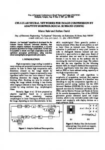
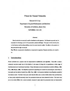
2.4.4 ADAM and AURA ADAM The ADAM network uses two binary CMMs in order to learn and recall associations between input and output patterns [41, 35]. An example of a CMM is depicted in figure 2.1. As we can see in figure 2.1a, a CMM uses a Hebbian like training method where the strength of the connection between two simultaneously active units is increased. pattern B 0
p a t t e r n
1
0
1
1
0
0
0
0
1
1
1
0
0
0
p a t t e r n
1 0 1 1
A
0 1 0 1 1
A
0
0
0
0
0
0
(a)
0
4
1
4
4
0
1
0
1
4
0
1
0
1
1
0
0
0
0
1
(b)
Figure 2.1: (a) Storing and (b) recalling in a binary correlation matrix memory. We can see in (a) that a connection between two simultaneously active units is set to 1.. For the case of a binary CMM this procedure is described as:
M�
�
� ��
A�
�
��
B�
�
�
where, M is a vector with
�
�
binary matrix,
� elements, B �
�
(2.1)
represents the OR function, A �
�
is the -th input binary row
is the -th output binary row vector with �
elements and � is the
number of input-output pairs. To recall a pattern from a CMM a matrix multiplication is performed between the input pattern and the matrix M (fig. 2.1b). In order to retrieve the corresponding binary pattern from the resulting
CHAPTER 2. ASSOCIATIVE MEMORY
20
array of integers a threshold function must be applied. This can be performed either by setting the sums above a value setting the
to 1s and the rest to 0s ( -threshold or Willshaw’s threshold method) or by
greatest sums to 1s and the rest to 0s. Deciding for the value of
is tricky when the
input pattern is distorted or noisy. However, if the output pattern has a constant number of bits set then we can use the latter approach ( -max method). The input-output pairs in ADAM are not associated directly. Instead, a sparse class pattern which is unique for every pair, has a constant number of bits set to one and is smaller than both the input and output patterns is used. Then, the input pattern is associated with the class pattern at the first CMM and the class pattern is associated with the output pattern at the second CMM. During recalling the input pattern is presented to the first CMM and one, or more, noise free class patterns are retrieved using the -max method. Applying the class pattern(s) to the second CMM the corresponding output pattern(s) is(are) retrieved setting as threshold the number of bits set at the class vector. The case of multiple class patterns corresponds to the case when two or more input patterns are superimposed. Then, the corresponding output patterns are to be recalled. An important feature of ADAM is the pre-processing applied at the input pattern. This is performed using the -tuple method where the input pattern is divided into groups of only one out of �
bits and
bits is set to 1 at the pattern after the pre-processing. The pre-processed
pattern is thus larger in size but has a constant number of bits set to 1 and these bits are more sparsely distributed. This affects at (a) classifying linearly inseparable patterns, (b) preventing fast saturation of the CMM and (c) facilitating the prediction of the performance of the system [41]. The use of binary CMMs and the -tuple method classify ADAM as a RAM-based neural network [37]. These networks are based on conventional digital hardware for their implementation and are generally characterized by speed both in training and recalling modes. ADAM is image processing oriented and is used in a variety of applications such as analyzing aerial photographs [42], feature and texture recognition [42] and, more recently, document image analysis [43, 44]. ADAM can also be used for grey level images by generalizing the -tuple technique [45].
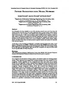
AURA The AURA [7] model derives from the ADAM network and is primarily oriented for symbolic processing. AURA is actually a set of methods for integrating neural and symbolic processing. An example of a possible configuration of the model as used by the system in this thesis is depicted in
2.4. THE NEURAL APPROACH
21
figure 2.2.
Antecedents (if P1 is A and P2 is B)
Tokenised Symbols
Lexical to Token converter
CMM
CMM
CMM
arity 1
arity 2
arity n
P1
P2
A
B
Superimposed separators
Binding
Superimposed tokens
Identify separators
Post−Condition Look Up (MBI)
Post−Conditions
Figure 2.2: The Advanced Uncertain Reasoning Architecture, AURA, model.
� �� AURA can handle symbolic rules of the form �������� � �
�
�� �� � � � . By precon�
ditions we mean a set of ���� ����������������� � pairs connected either with the logical AND or OR functions. An example of a symbolic rule is:
!�#"$%�&�('
��� � �*) �
�
The method which is used for converting the symbolic preconditions to a vector of input values is similar to the one used in [46]. However, binary instead of continuous vectors are used. The approach is based on tensor products production between binary vectors representing the variables and the values used. For example, if the variables and values used at the above symbolic rule are represented by the following vectors:
+ �
�
� �
��� � �
�
�-,
�
�
�.,
�
�
�
+
"/#� �
�
�
+ + �
�
�
�.,
�
�
�
then the final input is formed after superimposing the products is:
, �
� �
("/#� � and �
�
�
��� � and it
CHAPTER 2. ASSOCIATIVE MEMORY
22 � �
� � � �
�
� �
�
�
�
�
�
�
�
�
�
�
�
�
�
�
�
�
�
�
� �
�
�
� �
�
�
�
� �
���
� � �
�
� �
�
�
�
�
�
�
� �
�
�
�
�
�
�
�
�
�
�
�
�
�
� � �
�
�
�
�
�
�
�
� �
�
�
�
� �
�
�
���
�
�
�
�
�
�
�
�
� �
�
� �
�
�
���
�
� � � � �
�
�
As we will see, the form of the logical connection between the preconditions is achieved by setting the proper threshold value while the commutativity of the input arguments is supported by superimposing the produced tensor products [47]. After the final input vector is formed it is associated with a separator pattern at the CMM corresponding to the number of preconditions. This number is called the arity of the rule. The separator pattern has a role similar to the class pattern in ADAM. It is unique for every rule and it is a sparse binary pattern. During recalling, one or more separator patterns are retrieved using the -max method. These patterns can be superimposed in the vector retrieved. After an identifying process which gives a list of valid separators, these are then used as indexes to a database mechanism in order to retrieve the relevant postcondition(s). The database mechanism is based on the middle bit indexing (MBI) approach [48]. Depending on the number of bits set in each tensor product and on the form of the logical connection between the preconditions, a confidence test can be performed to the array of the summed values prior to the application of the threshold function. If a sufficient number of bits can be set then a vector containing one or more valid separators can be retrieved after the threshold process. More specifically, if the arity of a rule is �� , the number of bits set at each tensor product is
��
and
� the number of bits set at the separator patterns is , then, if the operator AND is used there must �
� in order to have a successful match of a be at least sums with value greater or equal to ����
�
� � rule. In the case of the OR operator this value is instead of �� � . It must be noted however
that the above values are the maximum expected. When inputs are superimposed there might be bits set to one sharing the same places. Thus, the values for the confidence measure could be less than the above ones. In order to handle this situation an option is provided in AURA where a line in the CMMs can be counted once or as many times as the number of bits which are superimposed in that place of the input pattern. The reason for using more than one CMMs at the first level is that handling of rules with different arity would be problematic otherwise [47]. For example if the rules
!� "/#� � ' �
�
� �&� �
)
2.5. ASSOCIATING RULES
�
23
�
��� � �
were stored using only one CMM and we wanted to find the relevant postcondition having only
�
���&� as input it would be impossible since both X and Y would be recalled. Thus, using a
different CMM for every arity we ensure that only the desired rules will be recalled. The AURA system provides partial match capability by altering the confidence threshold used and by accessing more than one CMMs. The way that this is applied in our case is described with more detail in section 7.2.4. Thus a postcondition, or a number of postconditions, can be recalled even if not all the necessary preconditions exist. This is a very important feature of the system and makes it a powerful and very fast search engine for uncertain reasoning and combinatorial matching problems. Both ADAM and AURA share a number of similar characteristics. The ability to operate in parallel on the data is one of them [49]. That means that simultaneous presentation of
input
conditions will result in recalling all the corresponding outputs. Additionally, the use of binary CMMs provides speed both at training and at recalling, enables the systems to perform on-line learning of associations and facilitates their simple implementation in hardware with C-NNAP [39] and PRESENCE [40] being the earlier and latest versions of the dedicated hardware platforms. It also provides generalization and noise handling abilities by allowing a flexible mode of operation depending on the threshold values and methods used. A more technical description of CMMs including both the cases when integer or binary weights are used is given in appendix A. Issues regarding the capacity and performance of CMMs are also referred.
2.5 Associating rules It was mentioned at the beginning of the chapter that associative memory is ideal for storage and retrieval of information represented by a relational structure [10]. This is because there is no need for complex indexing mechanisms and data constructions in order to handle the elements of the structure. Additionally, the use of associative information processing allows direct combinations of the existing knowledge and facilitates the inferring procedures. As we saw at the previous sections, connectionist models are able to provide powerful associative memory systems. Their noise and fault tolerance, the learning and generalization abilities and the distributed and parallel form of processing are the basic reasons for this.
CHAPTER 2. ASSOCIATIVE MEMORY
24
Combining these two facts and given the enhanced representational abilities of symbolic structures used in AI systems we come to the conclusion that we need a way to apply connectionist architectures for symbolic information processing. We are not the first to come to this conclusion. Combining connectionist systems with symbolic computation and design systems to support reasoning based on associations is an active field of research [46, 50, 3]. The basic approach that we are following in our system is that of the tensor product production [46]. This is applied at the basic symbolic processing level of the system which is performed by AURA. As we saw in section 2.4.4, the basic principle of this method is that variables and values are represented by vectors and their binding is represented by the outer products of these vectors. Using associative memories to handle symbolic information has a number of advantages compared to the use of conventional databases. The ability to handle efficiently a large amount of data is one of them. Traditional database systems do not scale well and have problems with large input queries and missing data. Slow operation and the increased amount of storage space needed are two examples. Moreover, noise at the inputs can make their operation problematic. The use of connectionist associative memories offers an alternative which overcomes these obstacles. However, slow training times, limited capacity, difficulties in hardware implementations and the problem of representing symbolic information in them were a source of scepticism. The AURA model described earlier offers a solution which is used in our pattern recognition system. Providing a fast and robust search engine, it offers at the same time partial matching abilities, parallel operation on inputs and on-line learning. These factors enable it to cope with the symbolic processing requirements of the system presented in this thesis.
2.6 Summary The aim of the chapter was to present the basic issues and models of associative memory, to concentrate in the model which is used in our system and explain why it is beneficial to use associative memories as the basic rule handling mechanism. An overview of the traditional software and hardware techniques for simulating content addressing and a brief survey of the neural network based methods for associative memory were given. As we saw, the use of connectionist associative models has advantages over the use of conventional methods. Ability to scale with the problem, fault and noise tolerance, generaliza-
2.6. SUMMARY
25
tion, speed of operation, parallel and distributed processing and representation are some of them. However, connectionist models may have limitations as well. Slow training, difficult and complex hardware implementation, costly operation and modest capacity are the usual problems. Using the AURA model of associative memory is a way to overcome these limitations and come up with a powerful connectionist solution for symbolic processing.
26
CHAPTER 2. ASSOCIATIVE MEMORY
Chapter 3
Cellular Automata 3.1 Introduction The generic model of a cellular automata system is probably one of the simplest models existing. A number of similar systems are arranged in a predefined space and each of these systems interacts with its direct neighbours following a set of rules. Although simple, this model can simulate many natural systems. In general, a cellular automata system consists of the cellular space and the automaton placed in each cell. The geometry of the cellular space defines the way in which the cells, or sites, are arranged and the kind of neighbourhoods that we can have. At any time instant the state of the automaton in each cell, or simply the state of each cell, is determined by its state and the states of the neighbouring cells at the previous time instant. Working on models of machines which would be capable of self-reproduction, John Von Neumann was one of the first people who introduced this term in the early 1950s [51]. Initially working on the design of a machine which would be able to reconstruct itself, he eventually came up with a model of self-reproduction using an array of computing elements. Each computing element was an automaton capable of being in one of twenty nine discrete states and they were all arranged in a rectangular cellular space in which they could interact with their direct neighbours in the four directions. Combining a number of these elements, more complex automata could be constructed and placed in regions of the cellular space. Providing a way to simulate a Turing machine, this cellular automata system was able to construct any automaton given its description. Consequently, it 27
CHAPTER 3. CELLULAR AUTOMATA
28
was possible to have automata-constructors able to reconstruct themselves or any other automaton in different regions of the cellular space. Probably the most well known example of a cellular automata system is Conway’s game of Life [52]. In that, there are two possible states that a cell can be in, dead or alive. A small number of simple rules specifies when the cells change from one state to the other and the system evolves in time starting at different initial configurations. Cellular automata are capable of complex behaviour and can be a model for several physical systems containing many discrete elements with local interactions [53]. Being sufficiently simple for detailed mathematical analysis they are also sufficiently complex to exhibit a wide variety of complicated phenomena. Using a synchronous and uniform updating model, i.e. application of the same rule set at the same time for all cells, under a simple direct connectivity regime they are indeed a paradigm for parallel and distributed processing. This chapter is a brief introduction and presentation of the model of cellular automata. The definitions of the terms used, a discussion about the different categories of cellular automata according to state and rules characteristics and the behaviour that the model is capable of and applications of systems with cellular structures, especially for image processing, is the main subject. At the end, a summary follows where having presented the basic ideas behind cellular automata we point out the enhancements at the general model which are introduced by our system.
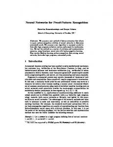
3.2 Basic definitions One important notion in cellular automata is that of the neighbourhood. For each cell in the cellular space, the states of the cells belonging in its neighbourhood determine its next state. Usually the term refers only to the surrounding cells while the term kernel is used when the central cell itself is also included. In one dimensional cellular automata we speak of neighbourhoods of radius composed from the cells on the left and the right of a cell. By convention, the sites at the edges of the cellular space have ‘virtual neighbours’ with value 0 or any other ‘neutral’ value depending on the state set used. Alternatively, they can be joined together giving a folded or cyclic form to the cellular space. In two dimensions, the most referred neighbourhoods are named after their initial proposer and thus we have Von Neumann’s, Moore’s and Golay’s neighbourhoods as depicted in figure
3.2. BASIC DEFINITIONS
29
3.1 Of course, it is possible for a neighbourhood to have variable size and shape depending on N W
C
NW N NE E
W
N NE W C E SW S
E
C
S
SW S SE
(a)
(b)
(c)
Figure 3.1: Three well known neighbourhoods in 2-D cellular spaces. a) Von Neumann’s, b) Moore’s and c) Golay’s or hexagonal. The central site is denoted with C and N,S,.. are used for denoting the site at the ‘north’, ‘south’, etc. the requirements of the application. Following the above examples, neighbourhoods in higher dimensional cellular spaces can also be specified. Having a neighbourhood defined, the state of each cell is decided according to a transition function or rule or transform. This function is applied synchronously in the ensemble of the sites in the cellular automaton. More formally,
� � ���
�
�
� �
� � � � � � � � ��� � � �
where,
� �
�
�
(3.1)
� � �
the state of site at time instant ,
��
��
��� � �
the coordinates of site in the �� space, the set of all non negative integers,
�
the dimension of the cellular space,
�� � N
the coordinates of the th neighbour of site � . N�� �� is the set of the coordinates of all the sites belonging to the
neighbourhood of � ,
the number of elements in N .
The function from � �
�
�
�
which is applied locally for every cell in the cellular automaton is a mapping
to � , where � is the set of the possible states each cell can be in. That is,
�
��� �
� �
� �
(3.2)
CHAPTER 3. CELLULAR AUTOMATA
30
This local transition function leads to a global mapping:
��� � �
(3.3)
where � is the set of all the possible configurations for the cellular automaton. In general, the operation in a cellular automata system is isotropic which means that the operation of the local transition function is not influenced by the location of the cell in the cellular space as long as the configuration of its neighbourhood remains the same. The number of rules in a cellular automata system is in direct connection with the size of the neighbourhood and the size of the states set. By applying a number of restrictions the number of rules can be reduced. The remaining rules are ‘legal’ as mentioned by Wolfram in [53]. One restriction is the quiescence condition stating that an initial configuration consisting solely of 0s, or the corresponding ‘neutral’ value, should remain unchanged. Another restriction is that rules should be reflection symmetric imposing that symmetric neighbourhoods should yield the same next state. The above two restrictions were applied in Wolfram’s one dimensional cellular automaton in [53] and [6].
3.3 Classifying cellular automata A brief presentation of the various categories of cellular automata according to cell characteristics (i.e. states and rules) and the behaviour of the model in general is given in this section.
3.3.1 Cell characteristics The states of a cell in a cellular automata system can be represented either with binary, continuous or discrete values. Binary values usually consist of one bit but in some cases they can use more bits. Of course in that case we can also talk about discrete states. However, the latter is used more for expressing states of a symbolic form. An example of this case is Neumann’s twenty nine states automaton. The states can also belong to a finite input alphabet set as is the case in [54] where cellular automata are used for language recognition. On the other hand, when the bits in the state are used as flags denoting the existance or not of an event we can talk about binary states.
3.3. CLASSIFYING CELLULAR AUTOMATA
31
An example of such states we have in the lattice gas arrays [55] where we have sites arranged in a lattice and each site communicating directly with its neighbours in six directions. In these systems, which are used for modeling the flow of fluids, each of the six bits expressing the state of a site declares the existance or not of a unit mass and speed particle moving in the relevant direction. As expected, continuous values as states are used when the information in the system is rather of a numeric nature. The coupled map arrays are an example in this case [56]. These systems, also called reaction-diffusion systems, are constructed in such a way as to correspond qualitatively to the solutions of the partial differential equations representing patterns growing under the action of repulsive and attractive forces (e.g turbulence, convection, etc). Image processing with cellular automata is also one case where we can meet continuous valued states for the cells. As far as the rules are concerned we have a number of categories which can sometimes coexist. Thus, rules can be totalistic meaning that the next state depends solely on the sum of the values of the neighbours. Conway’s game of Life is a typical example of a totalistic cellular automaton. Another classification for rules is as peripheral. This means that the state of a cell depends only on the values of the neighbours at the previous time step but not on the cell’s own previous state. The rules can be also deterministic or non deterministic. A deterministic rule yields a unique next state for each cell. Thus, using a deterministic transition function, a given configuration of a cellular automaton will have exactly one successor although it may have more than one predecessors. The non deterministic cellular automata, or indeterministic as mentioned by Burks in [51], are characterized by the fact that same neighbourhood configurations may correspond to more than one possible next states for a cell. A kind of indeterministic cellular automata are the probabilistic ones where each possible next state has a probability value assigned to it. The lattice gas automata and the coupled map arrays are two examples where probabilistic rules are used. Thus, a set of possible next states for a given neighbourhood configuration may exist and they are assigned various probabilities. Rules can also be fuzzy where the AND, OR and NOT functions which can be possibly used to describe the rules in a cellular automaton are replaced by their fuzzy versions (x+y, xy and 1-x respectively). Usually, cellular automata are characterized by irreversibility which means that the previous configuration of a cellular automaton cannot be found by considering the current one. However, when the global transition function is ‘injective’ the cellular automaton is reversible [57]. Margolus, in [58], gives the form that the transition function should have in order to calculate any
CHAPTER 3. CELLULAR AUTOMATA
32
preceding or any succeeding configuration knowing just the current and the previous configuration. Thus, knowing C � and C�� �
one could figure out C ��� �
or C�� � , where C� is the configuration
of the cellular automaton at time . Margolus also introduced the idea of block based or partitioned cellular automata [58]. In these, rule processors examine the contents of a block and then the entire block is updated according to the proper block rule. There are two different partitionings of the cellular space into blocks of the same size and the one or the other partitioning are used successively. This partitioning scheme is called the Margolus neighbourhood and using the proper block rules, or mappings, the evolution of the cellular automaton can be reversible. A system which is able to operate in this way is the CART which is a hardware implemented cellular array developed at the university of York [59]. An existing problem in cellular automata is the difficulty which characterizes the derivation of the proper set of rules for describing a set of observed behaviours (configurations). This is the so called backward problem or inverse problem. In a system which simulates patterns produced by chemical processes [60] a solution is applied using a genetic algorithm based search in the rule space. However, this is also one of the few cases that a rule production process is applied.
3.3.2 Behaviour Working with one dimensional cellular automata which had a kernel of three cells and two states per cell, Wolfram classified the behaviour of the corresponding rule space into four categories [61]. Cellular automata of these categories could: End up in a spatially homogeneous state (i.e. all 1s or all 0s) regardless their initial configuration (class I). Form a sequence of simple stable or periodic structures (class II). Demonstrate a disordered and aperiodic behaviour (class III). Yield complex localized structures showing a form of propagation (class IV). The alterations at the initial configuration as a result of the evolution of the cellular automaton and the effects that small changes at the initial configurations had at the evolution of the system suggested that “information” associated with the initial pattern propagated only a finite distance in classes I and II and could propagate an infinite distance in classes III and IV [6]. Cellular
3.4. APPLICATIONS
33
automata of class IV were conjectured to be capable of supporting universal computation having the appropriate initial conditions [6, 62]. The game of Life was shown to be capable of universal computation [52] as well as the reversible cellular automaton suggested by Margolus in [58]. Selforganization and the generation of self-similar patterns was also found to be a characteristic of complex cellular automata evolving from random or simple initial states respectively [53]. A more refined classification of the rule space of one and two dimensional cellular automata of various neighbourhoods and states per cell is found in [63] by Li et al. Statistical quantities such as entropy, mutual information and spreading rate of difference patterns were used for the classification of the rule space into regions of similar behaviour. The parameter used was the percentage of non-zero rules in the cellular automaton rule table. The evolution of cellular automata demonstrates that a small set of local rules applied repetitively on a large array of similar elements can result in a system with very complex behaviour. Most of the time the model of behaviour of a cellular automata system emerges as a result of its evolution and cannot be predicted due to the complexity involved. In a rather optimistic observation, Victor in [64] notes that Von Neumann’s twenty nine state cellular automaton suggests that an organ with behaviour as complex as the brain’s can be specified from limited genetic information. This suggestion is similar to Garis’s ideas about the construction of an artificial brain based on neural networks which will be ‘grown’ inside special cellular automata hardware under the control of a genetic algorithm [65, 66]. Either an exaggeration or a vision of things to come, these ideas demonstrate the potentiality of cellular automata to model complex behaviour.
3.4 Applications Due to their inherent parallel and distributed processing nature and the ability to demonstrate complex behaviour cellular automata have been used as models of physical systems. At the same time, their structure has made them suitable for image processing applications.
3.4.1 Modelling nature The initial motivation for the construction of the cellular automata model by J.V.Neumann was to find a way to simulate nature. Indeed, his twenty nine state model was capable of self-reproduction, in terms of producing a replica of itself in the cellular space. Later, Conway’s game of Life was
CHAPTER 3. CELLULAR AUTOMATA
34
an inspiration for many people to start thinking that complex behaviour could emerge by locally applying a number of simple rules. Being dynamical systems they can be used for modelling other dynamical systems with emergent behaviour. As Toffoli states in his thesis, “the importance of cellular automata lies in their connection with the physical world” [67]. Assuming that our world is computationally reversible, i.e. having all knowledge we can calculate what happened at a previous instant, cellular automata should be capable of demonstrating reversibility if they were to be considered as a model of the physical world. After proving that cellular automata could be reversible [67], Toffoli managed to remove that barrier. An example of using cellular automata to model and reconstruct patterns produced by chemical processes is given in [60]. As we mentioned earlier, a learning algorithm to extract cellular automata rules directly from the experimental data using a genetic algorithm to search in the rule space for those rules that represent the data best is also given. The emulation of snowflakes [68], the simulation of the motion of a flock of birds [69] and the modelling of flame patterns [70] are also some other examples in modelling nature with cellular automata. The lattice gas arrays and the coupled map lattices also belong to this category. More examples and studies of cellular automata exist in volumes 10 and 45 of Physica D. In all these cases, cellular automata always prove their place as a model of artificial life [71]. A model capable of reproducing some of nature’s acts on a computer’s screen.
3.4.2 Image processing Applications in image processing include a wide variety of transformations either local or global propagating. Transformations of both categories performed in the cellular logic machine CLIP4 are described in [72]. Edge finding, noise removal, image shifting, shrinking and expanding belong to the first category. An example of an edge finding local rule applied locally and synchronously for every pixel in a binary image could be stated as: “only black pixels with white neighbours will remain black at the transformed image”. Shifting could be easily done by each pixel propagating its value in the given direction while shrinking and expanding are two complementary tasks performed by removing or adding pixels at the outer layers of the objects. Other spatial operations such as high-pass (enhance sudden changes) or low-pass (remove sudden changes) filtering could also be performed using the proper templates [4]. The templates can be considered as weight matrices where each site’s new value is calculated by multiplying the
3.4. APPLICATIONS
35
values of the neighbours with the corresponding weights and summing the products. The template based approach is also used in Cellular Neural Networks (CNNs), introduced by Chua in [28]. CNNs are systems combining cellular automata with ideas from neural networks and are also primarily used for low and medium computer vision. Global propagating transforms are based on the fact that separate connected sets exist within an image. Thus, propagation initiated at a point or points on a connected set passes throughout the connected set to its borders allowing transforms to be applied to these sets as a whole. Being more complex and using more than one copy of the image, these transforms can perform labelling and counting of the objects in an image. A set of cellular algorithms for medium level vision problems such as gap filling, segment detection and template matching were also proposed by Pierre and Milgram in [73]. These algorithms have in common the notion of distance transformation where the values of the pixels are replaced by the distance from this pixel to the closest edge pixel.
3.4.3 Cellular machines Based in the idea of cellular arrays of processors a series of cellular logic machines were constructed starting from the early 1960s. CELLSCAN, GLOPR (Golay Logic Processor) and BIP (Binary Image Processor) were the first. They were primarily used for the application of basic image processing tasks (i.e. skeletonization, geometric transformations, etc) to binary images [5]. The next generation in 1970s and 1980s had machines with an increased number of processors controlled by a supervisor computer. The series includes machines such as the ILLIAC IV of the University of Illinois, the CLIP (Cellular Logic Image Processing) series at the University College London with CLIP4 having a Processor), the � �� �
�
array of processors, the �� �
�� DAP (Distributed Aray
� �� MPP (Massively Parallel Processor) and the CAM (Cellular Automata
Machine) [5, 74, 75]. Low level image processing operations, numerical and logical operations on two-dimensional arrays of data for solving problems in meteorology and operation research, computation of image statistics and two-dimensional discrete transformations are examples of the applications these machines were used for [5, 76]. Having a more flexible architecture, CAM by M.I.T was capable of implementing various cellular automata systems and it was designed so that each cell could have 2,4,8 or 16 states and up to 12 neighbours. The latest version of the machine, CAM8, is used in
CHAPTER 3. CELLULAR AUTOMATA
36
the ‘artificial brain’ project [65, 66].
3.5 Summary Either used for modelling physical systems or for image processing or just as a game, cellular automata always demonstrate their potentiality. They indeed show that a system composed of locally connected basic processing elements capable of applying a number of, relatively simple, rules synchronously in each site can demonstrate complex behaviour and have the ability for universal computation. Although having a local neighbourhood based communication, we can see examples of global propagation of information. Being a dynamic model they are also a paradigm of parallel and distributed processing. However, there are some limitations for the systems that follow this model. These are mainly focused at the difficulties to handle a large number of states and rules and the lack of an efficient learning algorithm to produce these rules. The system presented in this thesis has a cellular automata like architecture. Thus, the cellular space, the basic processing elements and the synchronous and local application of the same rule set are present. However, there are some differences from the basic model. These can be focused on the nature of the information being processed, the existence of an increased number of rules and states, the internal structure of the processors in each cell, the use of associative memories as search engines for the application of the rules and the existence of a simple but effective learning mechanism for producing the rules. These differences extend the capability of the classical cellular model of processing by introducing states belonging to different levels of hierarchy, a mechanism to produce the rules for the state transitions and the means by which the increased number of states and rules can be handled. The information in the system is of a symbolic rather than an arithmetic nature. The initial configuration comes from the initial labelling of the image, having symbols to represent geometric features. Although the global propagation of the information is inherent to the system due to its structure, it is assisted and refined by special modules of the processors. The rules are deterministic in their initial form but non-determinism can be inserted into the system during its evolution. However, this is handled by the associative memories and, as we will see later in the thesis, serves in aid of the purpose of recognition. Using the cellular architecture for our system except from having already the parallel and
3.5. SUMMARY
37
distributed nature of processing we also gain from the model’s evolutionary operation. Being a dynamic and evolutionary system, it manages to have a ‘virtual’ multilayred character. That is, in every iteration of the system the information therein is not only propagated but also represents the objects at different levels of abstraction. At the same time, the problem of recognizing an object has been reduced to recognizing small parts of it and connect the parts in every iteration until a complete description is available.
38
CHAPTER 3. CELLULAR AUTOMATA
Chapter 4
Computer Vision Architectures 4.1 Introduction Computer vision is associated with the computation tasks required in order to automatically obtain explicit descriptions of the physical world representations existing in images. Although vision is a task which is effortlessly performed by humans, the complexity and the vast amount of the required computations was soon revealed at the first steps in this research field. Being a cognitive process, vision is not a separated task but it is strongly related with other high level functions such as memory, recognition, learning, information encoding and representation, and reasoning. It is of no surprise then that, although being the subject of intensive research for the last decades, a complete understanding of the biological vision systems is still missing. With many anatomical and physiological parameters identified, the exact functions and connectivity of the modules involved are yet unspecified although a number of theories and models exist. However, among the facts which are already accepted are the existence of different levels of processing, the parallel nature of the operations involved and the existence of multiple communication paths [77, 78]. In an effort to understand and apply the mechanisms of human vision in order to build competent machine vision systems, research in computer vision has interdisciplinary links with psychology, neurophysiology and philosophy [79]. Being a vast area of research itself, it incorporates image processing, pattern recognition and artificial intelligence technologies. This chapter provides a very brief overview of the general aspects of computer vision in order 39
CHAPTER 4. COMPUTER VISION ARCHITECTURES
40
to discuss and analyze a number of computer vision architectures. This is in order to present some of the key ideas and approaches in the field and help deploying these factors that motivated our research.
4.2 Reasoning from visual information The information contained in visual representations of the world is multimodal. Of course, judging from our own perception of vision, this is not easily realized because when we are faced with this kind of information we can easily infer and extract the data and the information we are interested in without being aware of the underlying tasks that are taking place. For example, a simple glance at a road that we are about to cross suffices in order to decide our next move. The existence or not of vehicles coming within some distance limits is the main thing that we are interested in. The number of the cars, if any, their colour, their license numbers, the colour of the sky, the shape of clouds, the number of trees, other people or animals around, etc, all these are extra information existing in the image reflected in our retina. However, these are details that we usually do not remember or have completely ignored after a successful crossing of the road. In order to be able to reason from visual information a number of computational tasks at different levels is required. Their exact nature depends on the kind of information we need to extract from the visual stimuli. The above mentioned examples of the details that we can extract from a road scene are the results of the intermediate to higher levels of processing. Of course, the necessary input to derive these conclusions comes from the lower levels of processing. It is nothing more than natural then, that computer vision also employs different stages of processing.
4.2.1 Sources of visual information Before expanding in the processing stages we could spare some time discussing the sources of visual information and their relation with the data contained therein. A static image is one source. As defined in computer vision terms [80], an image is a spatial representation of an object, a 2D or 3D scene, or another image. It can be thought of as a continuous function
of two variables
defined on a bounded and usually rectangular area of a plane. The value of the image at spatial coordinates
��� ���
is denoted by
a small area around
��� ���
��� ���
and is determined by the response of a sensor sensitive at
. An image can be captured using photographic or video techniques and
4.2. REASONING FROM VISUAL INFORMATION
41
its digitization is necessary for its further processing. The digitized image is a two dimensional array of pixels (picture elements) and the value of each pixel responds to the light intensity in that location of the image. An image can be either coloured or grey scaled or black and white. Under normal lighting and physiology conditions, the images perceived by the human vision system are coloured ones. Of course, the colours depend on the kind of radiation which is fallen on and reflected by the objects. The human eye is only capable of perceiving a well defined spectrum of electromagnetic radiation which is defined as the visible wavelengths of light. However, using the proper equipment an extended range of radiation (e.g. X-ray, infrared, etc) can be used for capturing images. These reveal information inaccessible otherwise, e.g. skeleton pictures, heat emitted from objects etc. As it is natural, the amount of information contained in coloured images will be greater than the amount contained in grey scaled ones and these, in turn, will be a richer source than the black and white images. Of course, the amount of processing required and the storage space needed is in direct relation with the amount of information in an image. Depending on the lighting conditions and the clarity of the image, the information contained therein regards the shape and number of the objects, their nature and their relevant positions. Of course, this is only at a high level of abstraction. The term ‘nature’ is a very general one and can have many different interpretations varying from facial expressions to suggestions about the texture of objects. However, there are some kinds of information than cannot be always deduced without prior or extra knowledge. For example, the absolute dimensions of an object are not always deducible without a means of comparison. The latter can be the existence of another object with specified size in the same image. The same holds for the distance of the objects from the point which the image was taken from 1 . If the same unknown object is the only content of two images then it is possible to tell in which image the object was closer. However, it will not be possible to reason about the distance and the size of the unknown object if this is the only entity contained in one image. As mentioned, images can represent 2D or 3D scenes and objects. In the three dimensional case a complete description of the scene would require depth data about the objects. These are not always easy to deduce from a single image. Shading and texture are two factors that can be used to generate three dimensional descriptions from single images. Another option is to extend the source of the visual information and combine data from more than one image. These images 1
Of course, we suppose that the adjustment of the lenses remains constant.
CHAPTER 4. COMPUTER VISION ARCHITECTURES
42
would refer to the same scene or object as viewed from a different angle. This is the basic idea in stereo vision [81] where a matching process between the features of the one and the other image is initially required. Another source of visual information apart from the static images and the combinations of them is the image sequences. These are a series of frames grabbed at regular time intervals and they allow the study of the motion parameters related with the objects in the scene i.e how objects are moving in relation to other objects and the image capturing point. Depth and shape information can also be extracted from these images.
4.2.2 Processing stages Three stages of processing are usually involved in any machine vision system. The low, the intermediate and the high. The input to the low level is the actual viewer centered image which is what the image capturing device sees. The output of the high level is a world model which is based on the objects in the image and their relations. In order to proceed from the viewer to the world model a data reduction and compression process through abstraction is required. For example, a � � �
� �
grey scale picture of a car would have �
���
��� pixels each one having ��� possible
values. Having this input of ��� Kbytes, the output would be the type and other information about the car probably occupying less than � � or � � � bytes. Processing at the low level is pixel centered and the basic tasks performed are filtering operations such as noise and background removal and edge detection. The grouping of the edges identified at this stage and the formation of a higher level description whose basic elements are not at pixel but at a feature level is the responsibility of the intermediate level. At this stage a segmentation of the image is performed and regions existing in the image are identified. Edges are unified to form the boundaries of the objects and characteristics of other features, e.g length of lines, curvature, position, etc, are identified. This information is the input to the world model processing stage and the translation of these data to an object centered description is required. Knowledge about the world must be used in order to come up with a high level description from these data. Depending on how the world knowledge is represented, the object model has either to be derived or be the result of a successful match. In the first case knowledge exists as a set of rules, or productions, which have to be satisfied. In the second case, a set of expected world models exist and the task of the high level stage is to match the data provided from the previous stages of
4.2. REASONING FROM VISUAL INFORMATION
43
processing with one of these models. We can see now why computer vision combines image processing, pattern recognition and artificial intelligence. Commencing with image processing tasks, techniques from pattern recognition and notions from artificial intelligence must be employed in order to produce a result. As it is natural, a variety of approaches exist for each of the computational tasks at each stage. Of course, the exact nature of the processes and the kind of data that are used depend on the requirements of the problem domain. The boundaries between these processing stages are not strictly defined. Especially between the intermediate and the high level since it is often the case that the same or a similar idea is used but the kind of data which are processed defines the processing stage. Relaxation is an example. The aim of this technique is to derive an optimal interpretation of a set of data according to existing constraints. This technique, and its variations, can be used for segmentation (e.g grouping edges, defining boundaries and regions), labelling of lines in order to facilitate 3D descriptions, or, at a higher level, graph matching. The Hough Transform and its generalized form is another example. This method which is based on the transformation of the image data to a parameter space with the parameters defining characteristics of objects, can be used either for iconic to symbolic transformations [82] where basic features such as lines, curves, circles etc are identified or as the underlying methodology for high level object recognition [44]. Template matching, probably the most computational expensive method, is one more example. In this method the basic task is to match the input data with a template representing a known object. Either performed at a pixel level or using features of a higher level this method generally suffers from the very large search space which has to be examined. The large search space which was last mentioned is apparently one of the basic problems in intermediate and high level vision where tasks are of a pattern recognition nature. Either following a bottom up (data driven) approach where the basic features themselves suggest the possible world models or a top down (model driven) method where certain model hypotheses are validated on the basis of the existence or absence of the required low level features, the problem remains the same. Thus, the data reduction and compression process needs also to be augmented by the insertion of a dimensionality reducing factor in all the stages of the processing. Partitioning of the problem is the most intuitive approach. This is because it is easier to deal with many small scaled problems than with a larger one. Allowing parallel functioning towards a general solution care must be taken in order to benefit from the reduced dimensionality offered by the locality of the approach while
CHAPTER 4. COMPUTER VISION ARCHITECTURES
44
preserving global intercommunication and exchange of information. This is necessary in order to guarantee that the local solutions will build up the way to the global one. The above idea of parallelism and hierarchical processing is the general one. Parallelism can be applied in all levels from down the lower one to up the higher one. However, its nature will be different. As we will see at the next section, data parallelism is applied at the image processing level where the same operations can be performed in all the pixels at the same time. At the higher stages the problems are more of a classification and hypothesis creation and validation nature. Thus, a kind of parallel search to sets of models or rules will have to be performed. This will need the parallel operation of different tasks either on the same or in different data. Hence, this kind of parallelism is more complex than the previously mentioned one. The knowledge acquisition and handling is another parameter in computer vision systems. As it was indicated earlier, knowledge exists either as sets of rules that have to be satisfied or sets of world model instances. The use of rules implies a constraint satisfaction process which leads to consistent characterizations while the use of model instances involves a template matching approach. Knowledge has either to be inserted to the system by means of programming or be the product of a learning session. Of course, the latter approach is preferred as it leads to more flexible architectures compared to the more transparent but not easily adaptable systems of the former approach. The systems that are presented next are examples of architectures for image and scene understanding and object recognition. All of them are characterized by parallel and distributed processing either by means of arrays of processors or using connectionist architectures. The conventional parallel architectures offer generic and programmable hardware solutions to machine vision problems. At the same time neural networks provide their learning and self organizing abilities either to directly perform classification tasks or in aid, and enhancement, of classical methods.
4.3 Vision architectures 4.3.1 Associative processor arrays The use of arrays of associative processors, i.e content addressable processors, is a characteristic approach in most parallel vision architectures. These are SIMD arrays of simple processors which means that the same process is performed over a large set of data in parallel. The use of these arrays
4.3. VISION ARCHITECTURES
45
is usually focused at the low or intermediate vision tasks and the high level control is provided by more complex processors or a host machine. This control regards the nature of the tasks that have to be performed at the low levels in order to provide sufficient information for object matching or derivation using the knowledge about the world models which is available in some form.
Image Understanding Architecture The Image Understanding Architecture (IUA) by Weems et al [15] is a paradigm of a multilayered vision architecture. It consists of three levels of parallel processors where each level is distinctly different from the other two. Communication between levels is achieved via parallel data and control paths while the processing elements at each level can also communicate with each other in parallel. The first level of IUA is the Content Addressable Array Parallel Processor (CAAPP) which is a � � �
� �
array of 1-bit associative processors intended to perform low level operations.
The idea is to have one processor for each pixel of the image thus following the data parallelism approach. Operations performed at this level are edge detection, histogram formations, labelling of connected components, average and maximum values of pixels etc. The second level of IUA is the Intermediate Communications Associative Processor (ICAP) which is a �� �
�� array of
16-bit Digital Signal Processors. This is used for passing data and commands through the levels and also handles tokens (symbolic descriptions of image events) and supports data base functions that allow access to them. The highest level of IUA is the Symbolic Array Processor (SPA) which is an array of �� �
�� processors each capable of running LISP. A blackboard system is used for
the communication between the processes. The operations at this level include knowledge based inference and manipulation of object models while the lower layers serve as knowledge sources at different levels of abstraction. IUA is a knowledge based parallel architecture for computer vision. The existence of three processing layers is in accordance with the processing stages described at the previous section. Image processing algorithms can run in parallel at the first layer with intermediate control provided by the second layer. The higher level is used for knowledge based inference using a blackboard mechanism to allow communication and cooperation between the symbolic processors. Having the advantage of speed that the dedicated and parallel hardware provides, IUA tries to solve computer vision problems using typical approaches augmented by high speed processing. However, no self
46
CHAPTER 4. COMPUTER VISION ARCHITECTURES
adaptive ability is provided and object models and constraints must be programmed in order for specific tasks to be performed. Additionally, the ability of the system to generalize depends on the provisions made at the programming stage and is not an inherent characteristic.
Connection Machine Another example of a parallel architecture which can be used for computer vision tasks is the Connection Machine (CM). The Connection Machine provides up to 64K physical processing elements and millions of virtual processing elements and has the ability for multipurpose, reconfigurable communications networks. In contrast with IUA, this architecture is not dedicated for machine vision only but has also applications in other areas where data parallelism is useful [83]. Neural net simulation, protein-sequence matching, particle simulation, geophysics and computer graphics are some of the application areas. As far as computer vision is concerned, CM has applications in image processing, stereo matching and object recognition. One way that CM can be used for object recognition is described in [83] where object databases containing hundreds of models and parallel searching in each scene are used. In this scheme, image features in the scene serve as events and features of each model serve as expectations. Object hypotheses arise when ever an event satisfies an expectation. When a hypothesis is created a hypothetical instance of the corresponding model object is created and projected into the image plane. After that, a hypothesis clustering scheme is applied to order the suggestions by using support from mutually supporting hypotheses. Then, CM has to accept or reject thousands of hypotheses in parallel using a templatelike verification step where those having strong support for their expected features are accepted over those with little support. The method followed for object recognition in the CM is mainly a top down approach with influence from template matching. Initial evidence from the image is used and then a long scale search is performed. Although some effort exist to reduce the search space the number of potential matches is still large and the performance of the scheme relies on the fast parallel processing by the general purpose CM which has to be specifically programmed for that.
Heterogeneous Vision Architecture Having a layered structure similar to IUA, the Heterogeneous Vision Architecture (HVA) [16] is another computer vision architecture. However, instead of the fixed topology of IUA, HVA comprises four different types of modules that can be configured in a more flexible way according
4.3. VISION ARCHITECTURES
47
to the set of the vision tasks required. A layered structure is applied again providing parallelism in three different forms. The first module uses DSPs for linear filtering (convolutions). The second module is a 1D SIMD associative processor array for non linear filtering, morphological and other region based operations. A network of transputers is used for manipulating model databases and directing the operation of the other modules and the fourth module is a programmable frame store which intervenes between the above modules and is used for buffering the image data. Each module contains at least one transputer which directs the communication with the other modules. An example application of vehicle license plates recognition using HVA is discussed in [16]. In that, the associative array is used for a number of tasks. These are: adaptive threshold of the grey level image to a binary one, removal of small objects and smoothing, segmentation by region growing, determination of the bounding rectangles of the black objects in the image, acceptance of those objects having a suitable size and aspect ratio, resizing of the selected blocks to the same size as the reference characters, and, identification of the characters. The latter is performed using two different techniques. Either counting the number of holes and then comparing (template matching) the object with candidate reference characters or modeling a single layered neural network trained previously on the reference character set. All the above tasks are performed at the associative array processor under the control of the transputer network.
Semantic Network Array Processor
The use of associative processors is also found in the Semantic Network Array Processor (SNAP) [84]. SNAP is designed to deal with a number of artificial intelligence problems using semantic networks and markers for knowledge processing. With the nodes of the semantic network representing objects or concepts and the arcs representing their relations, markers are flags that can travel in the knowledge network following a number of propagation rules in order to group ideas and concepts. The application of SNAP to the problems of scene labelling and edge interpretation using discrete relaxation and stereo matching using dynamic programming is discussed in [17]. In that, the labeling problem is described by a semantic network and each cell in the associative processor array is allocated to each node of the network. First, the relations corresponding to initial labellings of the cells according to the set of constraints are stored in each cell’s content addressable memory. Then, the system tries to converge to the greatest consistent labelling by successively removing inconsistent interpretations.
CHAPTER 4. COMPUTER VISION ARCHITECTURES
48
SNAP is a parallel architecture designed to cope with problems in knowledge processing. Message passing and cellular processing are employed and semantic networks are used for knowledge representation. However, the architecture is intended to cope with the highest level of the problems leaving the preceding stages of processing to other sources.
4.3.2 Neural Networks As we saw in section 2.4, apart from being an example for parallel and distributed processing, neural networks also provide learning and self-organizing abilities. Various kinds of neural networks are broadly used with significant success for image processing and pattern recognition purposes [19, 85]. However, in most of the cases the neural networks are faced with problems of high dimensionality and large search spaces. This emanates from the fact that whole patterns or images are presented to them and they are expected to reach the correct conclusions. This results in the need for large sets of training samples and large networks as well. A possible way out of this situation is to employ alternative approaches and the systems we are about to see are some efforts in this direction. The first one regards the combination of two different neural architectures together and the next models are trying to integrate neural networks with other techniques such as relaxation and generalized Hough Transform (GHT). Moving within this framework are also the hierarchical feature extraction neural nets such as Fukushima’s Neocognitron [86] and Le Cun’s LeNet [87] which are also presented next.
Cooperating Neural Networks The cooperation of two different neural network models is the main idea in [88]. The first one is a variation of the MLP network and it is a layered model having successive feature extracting and averaging stages while backpropagation learning is used. The other network is a variation of Kohonen’s Self Organizing Map. In the derived model training is performed using vectors which include both the patterns and their association targets. After the clustering of the feature map during training, the units in the map are used to activate the correct output pattern. These two modules can be trained either separately or cooperatively or in stages. In the first case each module is trained separately, in the second case they are trained simultaneously and in the third case each module is partially trained and then they are combined and further trained.
4.3. VISION ARCHITECTURES
49
The combination of the two networks was based on the fact that they have different characteristics and thus their operation is based on different aspects. Hence, the first module incorporates local feature extraction and the second performs global template matching. The two modules are operating in parallel and their responses are either compared or, more effectively, form the input to a MLP network. In both cases the performance is better than the best achieved by one model only. However, combined training is difficult due to the difference in the conversion rates of the modules and geometrical invariance is not sufficiently resolved.
Relaxation with Hopfield net The use of a Hopfield like neural network for the constraint satisfaction problem of image labelling is suggested in [89]. The approach is based on the idea of relaxation and a methodology similar to the one followed for the Travelling Salesman Problem (TSP) by Hopfield and Tank is applied. Having a problem of
objects and �
labels, a network of �
�
units is created. The energy
function for the network follows the principles of the energy function for the TSP problem with the added influence of the set of constraints specified as binary and unary relations. The binary relations specify the adjacency or not of the objects in the segmented image as well as the compatibility of pairs of labellings for related objects. The unary relations specify characteristics of the objects such as ‘higher’, ‘moving’, etc and the compatibility of the labels for this kind of objects. The Hopfield net was selected because of its ability to converge to stable solutions. Indeed, following a weights modification algorithm with respect to the energy function, the network manages to reach low energy configurations corresponding to correct solutions. The problem is that in order to specify the set of the parameters effecting this procedure an ad hoc approach is needed and small alterations in these parameters can lead to incorrect solutions. Although the problem of ‘tuning’ exists, this approach is encouraging in the idea of applying neural networks for high level problems. However, it is only the self organizing and not the learning ability of neural networks that it is exploited. The set of constraints has to be externally generated and then provided to the network which in turn will perform the relaxation labelling as part of its converging procedure. At the same time, each image is a different case and needs a different set of constraints to be loaded without any reference to the previous images. A slightly different approach is suggested in [90] by Shipman. In that system, interconnected Hopfield nets are used to store the sets of constraints. In a simulation using only binary relations
CHAPTER 4. COMPUTER VISION ARCHITECTURES
50
between the nodes, where a node represents an object, their adjacency is represented by connecting them using a Hopfield net operating as a symmetrical associative memory. For example, having three nodes �
�
�
and
� where
�
is connected with � and � with
� , two symmetrical as-
sociative memories will be used and these memories will share the part for
�
. Starting with an
initial labelling of the objects, the labels are trying to reinforce each other in order to converge to a consistent solution. This system is an interesting approach including the ability to learn consistent labellings by storing the constraints in the local associative memories. The problem is that the set of objects to be labelled do not always have the same connectivity model and since they represent high level objects (e.g car, sky, grass, road, etc) a different network is required each time. For example, if the object represented by node
was also adjacent to �
a different arrangement
would be needed. Additionally, as it was indicated in chapter 2, the Hopfield net has limited capacity and problematic hardware implementation due to the full connectivity between the neurons. Although having the above problems, this approach is still a very interesting idea for combining neural networks with other techniques. As we will see in chapter 6, our system also uses the idea of interconnected associative memories, however, under a framework which overcomes the above problems.
Correlation Matrix Memories The previous approaches were three examples of how neural networks can be used for computer vision tasks. The first case is the most usual way in which neural networks are used. We referred to this system because of the combination of two models of neural networks for the same task. The other two approaches were trying to offer solutions to image labelling problems using the method of relaxation. Apart from handling problems at different stages only, the use of the above types of networks usually suffers from complex hardware implementation which is also necessary if the complete system is to be considered as a practical solution to computer vision problems. The systems that we examine next are trying to provide more complete solutions combining processing at more than one stage. The first one uses a GHT like method while the second one uses a relaxation approach. Moreover, they both employ Correlation Matrix Memories and specifically the ADAM and AURA models that were examined in chapter 2. Thus, they have already solved the problems of long training, capacity and hardware implementation. The methodology of the first approach refers to the combination of the ADAM network and
4.3. VISION ARCHITECTURES
51
the GHT for document analysis. In O’Keefe’s system [44], ADAM is used as a feature recognizer associating blocks of pixels with data structures containing the label of the object and the distance from the centroid of the object. Thus, objects are characterized by their set of features and the relative positions of them. During training, sets of features and relevant data structures are stored in ADAM. In the recognition mode, features are extracted from the image and the information from the associated data structures determines the object and its centroid’s relevant position. The relevant positions are used so that the labels are placed at the proper places in an accumulator array. After the feature extraction has taken place the labels stored at the accumulator array determine which objects exist where in the image. The object labels are binary and represented by bits of which only � are set. These vectors are added at each other at the locations of
vectors of
the accumulator array and the dominant label is determined after the application of the �� �
� �
threshold function. In a way, the operation at the accumulator array is similar to the second part of the Sparse Distributed Memory that we saw in chapter 2. The operation of the model as described above makes use of ADAM’s noise robustness and ability for generalization when a lower threshold is used. However, since features are directly related with objects and have no information about what their neighbours should be, the problem of excess false positives arises. In order to deal with that the operation of the system was extended so that features are identified by taking account of their neighbouring features as well. Moreover, in order to secure that locally consistent objects would also be consistent at a global scale, the feedback factor was introduced. This is because feedback allows the communication of information over a wider area than that of the local neighbourhood. In the feedback version of the above system each feature is associated with a set of triples
�
�� �
�
��� �� �� � �#� ��� � � in its neighbourhood. The � � � is the relative distance to the �
other feature, ��� ���� is the kind of that feature and � � ��� � is the class of the object that feature �
�
�
belongs to. Additionally, each feature of an object stores the number of its neighbours using another CMM. During recognition, two accumulator arrays are formed. One for the features and one for the object labels. Then, an � �
� �
threshold is applied to the accumulated data returning
the dominant feature(s) and object(s) at each position. In order to determine whether each feature has received enough evidence the number of the neighbouring units that it should have is recalled from the CMM and used as a threshold. If the accumulated evidence is the expected one, or a fraction of it, the feature remains in the features array. In the case that the new array differs from the previous one the above steps are repeated using the existing features as the new input. This
CHAPTER 4. COMPUTER VISION ARCHITECTURES
52
procedure stops when there is no alteration at the feature array. Effectively, the feedback model applies the relaxation algorithm in order to obtain a consistent labelling of the image. The set of the constraints are created and stored in the second CMM of the ADAM during the training stage. Pursuing a consistent labelling of the features, the introduction of feedback manages to reduce the number of false positives and offers better performance than the feedforward model when clutter exists. Alwis’ approach is somewhat different [91]. This system, intended for trademark image retrieval, combines classical preprocessing methods with graph matching using relaxation and associative memories. Initially an edge detection and segmentation phase is performed using the Sobel filter and contour decomposition. This initial feature extraction produces a list of straight line and arc segments along with their properties. This information is then used to obtain the perceptual relationships between the segments. The next step is to produce the Gestalt images where co-linear segments are replaced by continuous lines and co-curvilinear segments by continuous curve segments. Perceptual relationships are also extracted from the Gestalt images as well as characteristics of the closed figures from both the raw and the Gestalt images. Thus, a set of graphs is created from each image representing the relations of the features in the raw and the Gestalt image and relations of the closed figures in both cases. Information for each node of these graphs is stored in databases and the compatibility between the nodes of these graphs is stored in CMMs. When a new image is presented, the above process takes place again and the set of graphs corresponding to the new image is created. Each node is labeled with all the possible labels it can have according to the data existing in the database. However, the consistency of the labellings is not challenged yet. In order for a consistent labelling to be derived the information stored in the CMMs is used. This is performed with a way similar to the one used in [92]. Thus, the set of labels for each node is presented to the CMM which holds information about the specific kind of graph. The output is the set of node labels that the current labelling is compatible with. This set of labels is used as a mask in order to remove the inconsistent labels of the nodes which are connected with the node under investigation. The same happens for all nodes in all graphs. The derived labelling is consistent but not always unambiguous. Thus, more than one label may exist for a node. In the case that an unambiguous labelling is pursued the above step can be repeated and a higher threshold can be used for the output of the CMMs in order to limit the output set of labels. However, this added pressure to the process may sometimes result in loss of correct labellings while the convergence to an unambiguous labelling is not guaranteed [91]. Thus, the
4.3. VISION ARCHITECTURES
53
initial consistent labelling is usually preferred.
Hierarchical feature extraction The two systems presented earlier are based on the combination of the use of correlation matrix memories together with an evidence accumulation model such as the GHT or a relaxation based method. They both provide complete solutions in the sense that they start from the pixel level and continue all the way up to an interpretation of the image. Moreover, the use of CMMs facilitates their implementation using low cost dedicated hardware [40]. However, the first system has only two levels of labels (i.e. feature or object) and the second relies on an initial feature extraction process entirely with classical methods. The two systems which are presented next are examples of neural architectures based on the idea of hierarchical feature extraction starting from initial features and following the various stages of the hierarchy up to the complete objects. The first example is that of the Neocognitron [86, 93]. This model has a multilayered structure where the initial layer is the input one, the last layer is the recognition layer with cells corresponding to different objects and the intermediate layers are combinations of two sublayers of neurons called
��
and
. The first sublayer consists of groups of neurons which can detect different fea-
tures. All the neurons in one group can detect the same feature, however, in different places of the input image. Thus, each neuron in these groups has a local receptive field and neurons of the same group have the same spatial distribution on their inputs with the only difference that the receptive field is shifted according to the position of the neuron in the group. As far as the second sublayer is concerned its aim is to allow for positional errors in the input features. The same organization in groups exists and each neuron in a group receives signals from a group of feature extracting neurons which belong to the same category. A unit in these groups is activated if at least one of the feature extracting units is active. In the whole network there can be many alternate sublayers of feature extraction and positional shift toleration units and during this process local features are gradually integrated into more global features. The network follows a competition learning approach and its training is unsupervised in all the stages. As referred, the last layer is a collection of ‘grandmother’ cells each one corresponding to a specific pattern. The basic model of Neocognitron was initially having feedforward only communication paths but it was later augmented so as to incorporate backward paths as well [93]. That was in order to provide the function of ‘selective attention’ allowing automatic segmentation and recognition
CHAPTER 4. COMPUTER VISION ARCHITECTURES
54
of individual patterns presented simultaneously. Additionally, the model could then also restore imperfect patterns and eliminate noise. The second example, Le Cun’s LeNet [87], is somewhat similar. Again, layers consisting of sublayers of groups of neurons exist and the first sublayer in each layer is devoted to feature extraction. Local receptive fields also exist and an operation equivalent to a convolution with a small size kernel is performed by each neuron. Having the same weights for their input connections, the only difference for neurons extracting the same feature is the location of their receptive field. The second sublayer this time performs an averaging function and reduces the resolution of the first sublayer. Thus, weights from the first to the second sublayer are fixed and are all equal. A series of alternate feature extracting and averaging sublayers exist and apart from the first feature extraction layer different connectivity models may be used between the averaging sublayer units and the units of the next feature extraction sublayer. The output layer is again a set of units where each unit corresponds to a different object. The basic difference with the neocognitron model however is that error backpropagation and supervised learning is used. The above two systems utilize an important approach which is the hierarchical feature extraction and pattern formation process where more than two levels of features can exist and provide adaptive solutions for all stages of the process. However, they suffer from long training times, their operation is not trasparent to an external observer and they have a prefixed structure in the sense that always the same number of levels of hierarchy must be followed from a specific instance of their model.
4.4 Summary This chapter provided a very brief overview of the general aspects of computer vision and a presentation of a number of parallel architectures for image understanding and object recognition. As we saw, parallelism is necessary in order to deal with the computational load occurring in vision problems at all levels. Two kinds of parallel architectures were presented. The first one is based on arrays of content addressable processors at the lower stages. Higher level control is provided by programms running on more complex processors which supervise the arrays. These are knowledge based systems which can be programmed to perform various computer vision tasks. Providing complete solutions in some cases, the main problem with these systems is that they lack
4.4. SUMMARY
55
the ability to self adapt to their environment, their generalization ability is questionable and can be vulnerable to noise and errors. A different kind of parallelism is provided by the other architectures. Based on connectionist models, these models have simpler processing units forming networks with learning and self organizing abilities. Although having these characteristics, neural network models offer problem specific solutions and are usually faced with problems of high dimensionality which require large training sets. A solution in order to exploit the learning and self organizing abilities of neural networks while building a more general object recognition system is to integrate neural networks with classical techniques or follow alternative approaches in order to reduce the dimensionality of the problem. The last systems which were presented were steps towards this direction. Following the same notions, the system presented in this thesis attempts to provide an adaptive solution for shape recognition which uses neural networks at all stages and combines cellular information processing with ideas from structural pattern recognition.
56
CHAPTER 4. COMPUTER VISION ARCHITECTURES
Chapter 5
Rules and Structure for Pattern Recognition 5.1 Introduction There are two main approaches for pattern recognition. The decision-theoretic and the syntactic and structural approach. Decision-theoretic methods classify patterns according to a set of measurements of one or more characteristic attributes of the patterns. On the other hand, syntactic and structural methods rely on the structure of the patterns in order to classify them. The main hypothesis is that patterns consist of sub-patterns and formations of basic, primitive, elements. There is a hierarchy which is followed for each pattern. The complete pattern itself is at the top rank and the pattern primitives are at the bottom. In the space between, there are sub-patterns of higher or lower complexity depending on their place in this tree-like structure. The use of the structure of the patterns for their classification, requires that they are represented in a corresponding way. The main data structures allowing this representation are strings, graphs, trees, webs and arrays. The idea behind the use of these structures is that any information about the structure of the pattern and the relations among its subpatterns must be preserved. Thus a pattern is represented using a symbolic structure. Ideas from the formal language theory can be used for the classification, or, the methodology can be extended and other techniques can be used as well. Syntactic methods refer to the first case while structural methods refer to the second. String matching using string distance and nearest neighbour classification is one technique which 57
CHAPTER 5. RULES AND STRUCTURE FOR PATTERN RECOGNITION
58
belongs to the structural methods. Graph matching, and the problem of graph isomorphism, is an extension of these techniques to higher dimensional structures while Hidden Markov models can also be used.
The idea is whether we will try to match a pattern with one of a number of prototype patterns or if we will try to use the characteristic way with which patterns of a class are formed in order to classify the unknown pattern. Syntactic methods are following the second way. Patterns can be thought of as words in a language. These words consist of symbols representing pattern primitives. For each class of patterns, there is a set of rules defining their structure. Thus there is a grammar for each class of patterns and consequently the members of that class belong to the language which this grammar creates. An unknown pattern is classified according to the language it belongs to.
The advantage of structural and syntactic methods over the decision theoretic ones is that a description and classification of patterns in terms of their structure is achieved. That results in more complete understanding of the patterns by utilizing the relations among their basic components. However, decision theoretic methods have better behaviour in classifying noisy and distorted patterns and their algorithms are computationally inexpensive when compared with the ones for syntactic and structural methods [94]. Emanating from these facts is an endeavour for combining and unifying the two main approaches for pattern recognition. This results in the incorporation of attributes describing pattern primitives and their relations and the use of statistic methods and probabilities as an attempt to enhance structural based methods with error handling capabilities.
As the system presented in this thesis follows the guidelines of the structural and syntactic systems for pattern recognition, this chapter presents the basic notions and ideas behind these methods. These are presented at an introductory level providing the basic background for discussing the similarities and the differences between this system and other syntactic and structural based systems.
First the data structures which can be used for the symbolic representation of patterns are presented. Then, the basic tools and ideas for structural systems based on symbolic matching are introduced. After that, an introduction to the syntactic methods follows. Finally the chapter ends with a summary where a comparison between the presented methods and our architecture is attempted.
5.2. SYMBOLIC DATA STRUCTURES FOR PATTERN REPRESENTATION
59
5.2 Symbolic data structures for pattern representation As mentioned earlier, the idea of using symbolic data structures in order to represent the patterns is due to the fact that the information about the structure of the patterns must be preserved. Strings are the simplest data structure that can be used for the symbolic representation of patterns. A string is a word of arbitrary size composed by symbols of an alphabet. In the case of syntactic and structural pattern recognition this alphabet is the set of all the symbols representing the pattern primitives which are used for composing the patterns we are interested in. An example of a string representation of a pattern can be seen in fig. 5.1 a
b
c
Figure 5.1: A symbolic representation of a pattern using a string of symbols. The pattern can be represented as ������� ������� ��� ��� ��� . Having the alphabet of symbols, � , the patterns can be considered as possible words over � .
The set of all possible words over � is represented with �� . There are subsets of �� where all their members are following a number of rules. For example, the set of all strings having the structure
� � � ��� �� ��� . These rules are specified by a grammar,
� called a language produced by
,
� �
�
, and the corresponding subset of �
is
. Although more details can be found in section 5.4 it is
easy to imagine that a class of patterns sharing similar structural characteristics can be described by a grammar and represented by the corresponding language. Thus, in a perfect world, all that somebody has to do in order to classify an unknown pattern having its symbolic representation is to find out which language it belongs to. Another way is to compare the unknown pattern with a number of prototype patterns in order to classify it. This form of comparison can be performed using a kind of distance metric and it is called nearest neighbour classification. Other methods for symbolic matching, e.g search for isomorphisms, can be applied as well. Whatever way is used for the classification of patterns having their symbolic representations, when strings are involved the algorithms are the simplest compared with other symbolic data structures. However, strings are inherently one dimensional and thus there are limits in their descriptive power. The relations between the pattern primitives represented by symbols in a string are usually confined to the type of ‘followed by’ or ‘precedes’. Of course, and as K.S.Fu notes in [95], there is an interplay between the complexities of the pattern primitives and the descriptive power of the
CHAPTER 5. RULES AND STRUCTURE FOR PATTERN RECOGNITION
60
symbolic structures with an extension to the complexity of the relevant pattern grammars. Thus, using more sophisticated pattern primitives we can increase the descriptive power of the symbolic structure. But then we need a more ‘expensive’ system for producing these representations. Another way to increase the descriptive power of strings is to use the Picture Description Language (PDL) [96]. In that, four binary and two unary operators are introduced. Pattern primitives now have two connecting points, a head and a tail, and by using these operators more complex patterns can be described. An example of using this method is the system in [97]. Extending this idea to more concatenation points at the primitives we have the plex structures and the plex grammars [98]. A more powerful method for representing structural information is by using graphs. Relations between pattern elements, existing in two or higher dimensional space can be directly represented using this structure. A graph consists of a set of nodes and edges connecting these nodes. Usually, the nodes represent the components of a pattern and the edges represent the kind of relations existing between those components. The nodes in a graph are usually labelled. A name that can be found in the literature for this kind of graphs is webs. When the edges in a graph have directions then we have a directed graph. Using graphs more complex patterns and scenes can be symbolically represented. In a direct analogy with strings, graph grammars and methods for classifying graphs using graph distance exist. When there is a direct mapping between the nodes and the edges of one graph with the nodes and the edges of another graph there is an isomorphism between the two graphs. The trade off for the descriptive power of graphs is that they are computationally expensive. A structure less complex than graphs and yet more powerful than strings is the trees. By analogy to trees found in nature, a tree has (1) a root, (2) a number of intermediate nodes and (3) a number of terminal nodes, leaves. The root has only outgoing links, the intermediate nodes have exactly one incoming link and a number of outgoing links while leaves have only one incoming link. Trees can be used for hierarchically describing a pattern having the complete pattern as the root and the pattern primitives as the leaves. The intermediate nodes represent sub-patterns which can be formations of pattern primitives or simpler sub-patterns. A study of matching tree structures is given by Sanfeliu in [99]. Another data structure that can be used is that of arrays. In an array, a placement of nodes into rows and columns is followed. Thus, following either a four-neighbourhood or an eight-
5.3. SYMBOLIC MATCHING
61
neighbourhood approach, a node is directly related with its four or eight neighbours in all directions. Hexagonal arrays can also be found where a slightly different approach is followed and each node is directly connected to six other nodes. Arrays can be thought of as the direct extension of strings to two dimensions. Again, array grammars and array matching methods exist for the classification of array represented patterns. An example of using arrays to represent patterns is the system presented in this thesis. The common characteristic of the above data structures is that they all describe relations between the primitive parts of patterns. Moreover, strings, arrays and trees can be thought of as special cases of graphs. Actually, a graph is itself a special case of a relational description [100] where there are only binary relations among the basic parts of the entity which is described. To make things simple, if we consider a set � of the symbols representing the parts of an entity, then any subset
of the Cartesian product �
-tuple in an -ary relation
� �
�
�� ���� � � �
� � is called an -ary relation over � . An
�
over � represents a relationship of some kind among the elements �
of the -tuple. A relational description , the parts of the entity. Thus, �
��
�
� �
��
�
, of an entity is a set of relations ������� ��
� �
�
over the set � of
�
.
The descriptive power of relational structures can be augmented by the use of vectors of characteristic measurements, or attributes, describing the pattern primitives or/and their relations. For example, the description of a basic pattern primitive, e.g. a line segment, can be augmented by using information as length, declination, etc. This results in having attributed symbolic representations which can provide enhanced descriptions of the patterns.
5.3 Symbolic matching The structural methods classify a pattern comparing its symbolic representation with a number of prototypes. As it is referred in [94], structural methods are more preferable than the syntactic ones when the number of prototypes is relatively small, the knowledge about their structure is not complete and the patterns of each class are not characterized by specific structural similarities. A metric which is widely used in structural methods is that of the distance between symbolic representations of patterns. In the case of strings, the distance between two strings � and � , with � and �� �
, is defined in terms of the transformations required to derive �
from � [101, 95]. The
transformations, or edit operations, are basically substitutions, insertions and deletions of symbols
CHAPTER 5. RULES AND STRUCTURE FOR PATTERN RECOGNITION
62
in the strings. Usually, there can be more than one way to transform �
into
with a different sequence of �
transformations followed each time. By assigning weights to each edit operation, each of these sequences is characterized with a cost. The minimum cost of all the sequences to transform � into �
is defined as the distance �
��� ���
between � and � .
Based on string distance the classification of patterns can be achieved using the nearestneighbour (NN) method or the
nearest neighbours ( -NN) method. A threshold can also be
added for the classification. Thus, having the class � with patterns �� �� � � �
��� � � �������
and defining � �
�
�
���
�
���
�
� �
���
�
� �
�
�
and � � ��� ���
�
with patterns �
��� ���
�
� �
�
���
�
��� � � ��� �
�
and class � �
as
���
� ��
�
�
����� � � � ����� � � � �
we have that
�
� � �
�
if
�
� �
�
�
���
� � � �
�
�
�
�
�� ���
�
When a threshold is added the distance must be also less or equal to that threshold otherwise the unknown pattern is rejected. In the case of the average of the distances of the
neighbours, the distance from a class is taken as
closest to � elements of that class.
The basic method which is used for computing the distance between two strings is a dynamic programming algorithm proposed by Wagner and Fischer [102]. This algorithm calculates the weighted Levenshtein distance as it is known and has a space and time complexity of � and �
�
�
where
are the sizes of the strings. The sequence of the edit operations needed is also produced
by this algorithm. Improved versions of the algorithm with reduced time and space complexity can be found in the literature [103, 104, 105]. A different approach using the Hamming distance has recently been proposed in [106]. It encodes the strings as binary patterns and produces a distance which is equal to the corresponding Levenshtein distance. String distance can be used as a tool for clustering the pattern space. In the pattern classes produced, the maximum distance between a pattern and others belonging to the same class must be less than the minimum distance between this pattern and patterns of another class. An extension to classical string matching is the elastic string matching where
appearances of the same symbol can
5.3. SYMBOLIC MATCHING
63
be ‘compressed’ to one and vice versa. Some applications of string matching include recognition of 2-D shapes [107, 108], seismic pattern recognition [109], handwriting recognition [110, 111], combinatorial pattern discovery in protein databases [112] and phonetic string matching [113]. The use of string distance is a basic tool for structural pattern recognition. When more complex data structures are involved (trees, graphs, arrays) the notion of distance can be extended. This is achieved by the use of more complex edit operations which include substitutions, insertions and deletions not only of nodes but of edges as well. An overview of how the notion of distance is applied for tree matching can be found in [99]. Another method for structural matching is by using the notion of isomorphism. Graphs and trees are the data structures which are mainly used in that case. Informally, a graph is isomorphic with another graph when there is a direct mapping between the nodes and the edges of the one with the nodes and the edges of the other. When a graph graph � there is a subgraph isomorphism between Having a graph �
with �
�
�
is isomorphic with a subgraph of another
and � . The same also applies for trees.
nodes and a graph � with � nodes, a first attack to the problem is
to construct a search tree trying to find mappings between the nodes of the graphs. The problem is that this method has a computational time complexity of �
��� � �
[101]. Using Ullman’s rule [114]
the size of the search tree can be reduced. This rule says that if node node �
of graph � and there is a relation between nodes �
and � � � of
of graph �
�
is mapped to �
� , then, if node � is � � of
a possible mapping of ��� there should be the same kind of relation between nodes �
� and � . � � in
In this approach, a future error table, FET, is created having a row for each node of graph a column for each node of graph � . The table has binary values and FET(� node � of �
can be mapped to node �
���
�
and
) = 1 means that
of � . After the initialization of the table and after the first
possible mapping of nodes, FET is updated and the search continues for the remaining nodes of �
. An incoherent mapping (� � � ) will make the updating of FET impossible so the next possible
mapping for node � is checked. If an isomorphism between end when all nodes of �
�
and � exists, the procedure will
have been successfully mapped to nodes of � . If it is necessary, the
algorithm can be continued until all possible mappings for all nodes have been checked. Actually, the above algorithm is an application of discrete relaxation where both possible interpretations of parts and constraints are set using Ullman’s rule. Shapiro and Haralick refer to it in [100] as backtracking tree search with forward checking. An approach based on the idea of graph and subgraph isomorphism and having as a tool the
64
CHAPTER 5. RULES AND STRUCTURE FOR PATTERN RECOGNITION
graph distance metric is that of inexact graph matching. In that, one graph is considered as a distorted version of the other and the level of similarity is expressed by the number of edit operations needed for obtaining a mapping of the elements of one graph to elements of the other. Combining the above approach with the use of attributed graphs is the system in [115]. In that system the calculation of the distance between the graphs is based on their decomposition in basic graphs and the use of a dynamic programming technique [116]. Another method for error-correcting subgraph isomorphism detection is based on a network representation of the graphs while incorporating edit operations [117] .In that, identical subgraphs of the model graphs are represented only once and the necessary number of steps to detect exact and inexact subgraph isomorphisms is reduced. The main disadvantage of subgraph isomorphism detection and inexact graph matching is that it is a NP-complete problem and has an exponential time complexity. As a possible way to overcome this, a number of stochastic optimization methods including probabilistic relaxation, simulated annealing and genetic algorithms have been applied [118]. They have a polynomial time complexity but the optimum solution is not guaranteed. On the other hand, combinatorial search methods need to be augmented by heuristics restricting the search space.
5.4 Syntactic methods As we saw in the previous section, the structural based methods use a ‘one to one’ comparison between the unknown pattern and the prototypes. However, when the number of the prototypes is not small this comparison could be a drawback. Additionally, there might be the case where structural similarities exist among the patterns of each class. The most appropriate method to be followed in that case is to, somehow, ‘store’ the structure of the patterns of each class in some form and then search which form the unknown pattern is coherent with. One approach is to use Hidden Markov Networks [101, 119]. Then, one representative model is generated for each class and probability distributions are used in order to handle the variations among the patterns belonging to the same class. Another approach is to use the notions of grammars and languages from formal language theory. In that, structural information is encoded as rules, or productions, of a grammar and each class has its own grammar representation. The latter approach is the basis of the syntactic pattern recognition. In the following paragraphs basic concepts from formal language theory are briefly introduced and their application for pattern recognition is presented.
5.4. SYNTACTIC METHODS
65
5.4.1 Basic formal language theory As it was mentioned in section 5.2, having a set, or alphabet, of symbols, � , the set of all possible sentences over � is represented with �
. This set is called a closure over � and also contains the
empty string, , which is a sentence with no symbols. The set represented with � �
positive closure over � and it is �
� �
� � . Any subset of �
�
is called a
is called a language over � .
A grammar, as is defined in formal language theory [120], is a four-tuple
�
� �
" �
�
��� �
where, is a finite set of non-terminals,
"
is a finite set of terminals, �
is a finite set of productions of the form � ��� �
is a starting symbol ���
and �
� � and � "
��
�
and " is the null set while their union is represented with � . That
The intersection of sets is, "
�
�
is of the form � ��� where � ��
��� . Any production �
. The productions represent ways of rewriting sentences of �
�
non-terminal exists, to sentences in �
��
,where at least one
. There are no rules for rewriting combinations of terminal
symbols only. Thus, starting from symbol � and following the set of productions in
�
, after a
number of rewritings we end up with sentences containing only symbols from " . The derivation of � starting from � and following a series of productions is represented as ���
in
�
The subset of "
�
.
containing sentences over " which are created according to the productions
is called a language created by grammar �
�
�
�
and is represented as �
�
�
"
�����
�
�
. Thus,
� �
Grammars can be classified to four categories according to their productions. When there are �
no restrictions to the form of the productions in productions are of type
� � �
�
��� �
where �
the grammar is called unrestricted. When the � �
���
��
and � ��
�
the grammar is
called context sensitive. This is due to the contextual prerequisites which exist in order for the productions to be applied. A context free grammar has all its productions in the form with form
� �
� �
���
��
or �
�
�
� �
. Finally, a grammar is called regular when the productions are of the
�
� where �
�
and �
" . The above classification is known as
the Chomsky hierarchy. It must be noted that regular grammars are a special case of context free grammars, context free are a special case of context sensitive and context sensitive are a special
66
CHAPTER 5. RULES AND STRUCTURE FOR PATTERN RECOGNITION
case of unrestricted grammars. Grammars are also called as of type 0,1,2,3 from unrestricted to regular respectively. This type of classification is also used for the languages according to the most restricted grammar which can create them. The type of grammars mostly used in syntactic pattern recognition are the context-free and the regular ones [101]. The above definitions are presented in a string oriented manner. However, they can be extended for higher dimensional data structures like trees, arrays and graphs. The additional requirement is that productions should now be enhanced with specific descriptions for their application. For example, in a graph grammar where rewriting rules may exist for replacing a subgraph �
with
another subgraph � , the relevant production should also specify how the nodes of � should be connected with the nodes adjacent to �
.
One more concept in formal language theory is that of the automaton. An automaton can be thought of as a mathematical model of a computation machine [121]. In its general form it is a state machine and it is characterized by a set of states, a set of input symbols, a set of output symbols and a set of mappings between combinations of input symbols and states to output symbols and states. One aspect of automata which has special interest to syntactic pattern recognition is that they can act as recognizers of languages. That is, having as input a sequence of symbols they can decide, in general, whether that input belongs to a specific language or not. Among the different types of automata we can distinguish the finite state and the push-down automata for their ability to recognize regular and context-free languages respectively. A more direct way to decide whether a sentence of symbols belongs to a specific language or not, is to attempt to construct its derivation tree according to the productions of the relevant grammar. If the attempt is successful then the sentence belongs to the language. A derivation tree is a tree having as root the starting symbol, nodes from the set of non-terminals and leaves from the set of terminals. For each node and its offspring(s) in such a tree there should be a production having the node as the left hand part and the offspring(s) as the right hand part. The procedure of constructing the derivation tree, and effectively finding the productions sequence to be followed for the construction of a sentence � , is called parsing of �
according to grammar
�
. Parsing
can follow either a bottom-up or top-down fashion. The former starts from the actual sentence of terminals and proceeds by reverse applying the productions trying to reach the starting symbol. The latter starts from the starting symbol and proceeds by applying the productions aiming to the reconstruction of the input sentence.
5.4. SYNTACTIC METHODS
67
Depending on the options available at each stage of the rewriting process, a grammar can be classified as deterministic, non-deterministic or stochastic. In a deterministic grammar there is only one option available at each step. That is, there are not two, or more, productions having the same left part and different right part. Thus, rewriting proceeds with well determined steps at each time. In a non-deterministic language, there might be more than one possible steps to be followed when applying the rewriting rules. Whether one or an other production will be applied depends at the specific case. Thus, the decision to apply a specific rule could be right at one case and wrong at another. At the latter case, when the wrong rule is applied, backtracking might be necessary. A similar situation, more than one available productions, exist in a stochastic grammar. However, each production in that case has a probability value assigned to it. This value represents the frequency with which the rule is used when deriving the sentences of the relevant language. In the case of a stochastic grammar each derivation is characterized by the product of the probability values of each production used. It must be noted at this point that it is possible for a sentence to be derived with more than one sequence of productions. This is characteristic of an ambiguous grammar.
5.4.2 Syntactic recognition For the application of formal languages theory to pattern recognition the set of terminals corresponds to the pattern primitives, patterns are symbolically represented by means of a relational structure and a grammar is associated with each class. Non-terminals represent more complex formations of pattern primitives or repetitive structures in the patterns. However, as Tanaka notes in [122], their meaning can be more abstract or indirect.
Parsing
� it must be possible for it � to be parsed according to the underlying grammar � . Some well known string parsing methods
In order for an unknown pattern to be classified as belonging to class �
are the Earley’s [123], the CYK [124], and the direct parsing [125]. The first one is a top-down method using lists and the second is a bottom-up approach using triangular tables. In both of them, a successful parsing is characterized by the existence of a node or a cell containing a specific value after an iterative procedure. As the name suggests, direct parsing is following a different approach trying to construct the derivation tree directly. This method includes backtracking when necessary.
CHAPTER 5. RULES AND STRUCTURE FOR PATTERN RECOGNITION
68
Since most patterns are not presented in a perfect and noise free form, the parsers should include error handling capabilities. In Earley’s method this is implemented by the use of the covering grammar [101]. This is the basic grammar model augmented with productions necessary for the error correcting transformations, i.e. substitution, insertion, deletion. Using the covering grammar the parser always ends up with a solution. Moreover, a number is also produced as a result of the transformations that need to be applied to the input pattern in order for it to be accepted from the original model. Nevertheless, the use of the covering grammar, which is more extended than the original one, has a negative effect in the time and space needed for parsing. A different extension of the Earley’s algorithm for error correcting parsing without the use of the covering grammar along with other string parsing and error correcting parsing methods, which are more or less variations of the basic ones, are presented in [126]. Some ideas for parallel parsing and VLSI implementation of extensions of the basic model of the Earley’s method are presented in [127]. Combining the error correcting parsing methods and the notion of the distance between patterns, as referred in section 5.3, the distance between a pattern and a language can be introduced and used for the classification of the input patterns. When a more extended representation ability is required strings are not always adequate. Thus the use of higher dimensional structures is necessary. Trees can be used as a first step. An example of a fingerprint recognition system using tree grammars and automata is presented in [120, 128]. Graphs are the next generalization. Due to their extensive description power, they have been widely used for pattern representation. However, the parsing of graph structures using graph grammars has not been an easy problem [129, 130]. That is one of the reasons that the use of plex structures and picture description languages were preferred [131]. One case where graphs can be applied for syntactic pattern recognition is when some restrictions are imposed to the general graph grammar model. Then, algorithms can be constructed for parsing and error correcting parsing the resulting grammars. Such an approach is presented in [130] and is tested in industrial robot control systems. A variation of the conventional graph grammar model is presented in [129]. The model is extended by controlling the application order of the productions and augmenting the nodes and edges with attributes. Additionally, instead of parsing the input graph a transformation of it to an output interpretation takes place. The transformation is guided by the productions of the grammar when applied according to a specified sequence provided by a control diagram. If an output interpretation of the input graph is not possible then the input is rejected. Thus, instead of constructing
5.4. SYNTACTIC METHODS
69
a hierarchical description of the input pattern this is transformed to its highest level representation. An application of this model to circuit diagram and flow chart recognition is also presented in [129].
Grammatical inference A very important issue in syntactic pattern recognition is that of grammatical inference. That is the derivation of a grammar given an example set of patterns. The example patterns belonging to the language that the unknown grammar should generate are called positive examples. Examples not belonging to this language are called negative. A basic theoretical aspect in grammatical inference and a criterion for the successful learning of a language is that of the identification in the limit [132]. Simply stated, identification in the limit of given a set of positive, �
a language
� �
that
�
� �
�
� �
�
and, �
��
to sample sets of increased size, it is
�
, and negative examples, �
� � �
� �
� . Moreover, for grammars �
���
�
� �
�
such
corresponding
. According to Gold in [132] we have two
� �
fundamental results. The first one is that for every grammar
� , �
�
, is finding a grammar
in an admissible class of grammars,
is identifiable in the limit by a structurally complete sample of both positive and negative
examples. Two necessary definitions are the following: (1) A class � admissible when it is denumerable and for every
� not for any �
in �
while (2) a positive sample �
�
�
in "
� �
of grammars
it is decidable whether
is called
�
�
is called structurally complete when
� � �
or its
� vocabulary (set of terminals used) is the same as the one of the unknown grammar and � � each production in is used at least once for the derivation of the patterns in the sample. The
second result is relatively negative in nature and says that for an admissible class �
� �
generating finite languages
� � , if � �
language
� � � ���
then
� � � ���
� has at least one grammar � ���
of grammars
generating an infinite
is not identifiable in the limit through positive examples only.
The majority of the grammatical inference methods refer to regular grammars. This is justifiable by the fact that although regular grammars have the least description power compared to the other grammars of the Chomsky hierarchy, they are the easiest to operate with. The notions of canonical grammar/automaton and of the derived grammar are common place in regular inference. A canonical grammar
� grammar
�
�
produced by sample set �
� derived from a canonical grammar
�
is the one for which �
�
� �
�
. Any
by partitioning the set of non-terminals into
equivalence classes is called a derived grammar and it is �
�
�
�
�
. The set of the derived
CHAPTER 5. RULES AND STRUCTURE FOR PATTERN RECOGNITION
70
grammars defines the set of potential solutions we are looking for and focus moves to finding the optimal one. The problem is that the number of derived grammars of a canonical grammar
�
is
in analogy with the number of symbols in the alphabet of the complete sample set used for creating
�
. We limit ourselves in saying that this number is � �� and � � �� for 10 and 20 symbols
respectively [133]. A formal discussion about the search space of the regular inference is given in [134]. The basic methods for regular inferencing are described in [135, 136, 120, 133]. Most of them are based on inferencing a canonical automaton from the sample set and then minimizing the derived regular grammar. The identification of regularities in the sample set and the use of � -tails1 are amongst the basic techniques used. The use of recurrent neural networks (RNNs) in
order to learn regular grammars using positive and negative samples has also been reported [137] and hybrid systems combining neural processing with symbolic representation and processing exist [138]. Some problems connected with this case include the possibility of bad generalization, failure due to local minima and insufficient control of the induction process [139]. Context free grammars have better description power than the regular ones and are more complex. Unfortunately, so is the problem of their inference. The majority of the methods are referring to subclasses of context free grammars and some of them are extensions of the methods for the regular grammars. The inference with a help of a ‘teacher’ answering queries for discovering nesting or recursive structures in the positive sample, the use of precedence relationships on the elements of the sample and constructions such as the pivot grammars are the most referred techniques and heuristics [135, 120, 133]. Lately, the augmentation of the words of the sample with their unlabelled derivation trees has also been suggested and used for inferencing context free grammars consistent with the samples [140, 141, 142]. Moving to higher dimensional grammars we find methods for inferring tree and array grammars. The basic principles for grammatical inferencing and similar heuristics are again followed. However, they are extended to meet the higher complexity of the multi-dimensional structures [143, 133, 120]. An attempt to construct a mathematical basis for the tree inference methods is presented in [144] while a method for inferring context free array grammars is presented in [145]. In the case of stochastic grammars the assigning of probability values to the productions of the inferred grammar is also required [133, 120, 143]. One way to estimate these probabilities is to calculate the relative frequency by which each production is applied to generate the example patterns. Of course, this method requires that the productions themselves are already known and 1
The � -tail of � with respect to the set of patterns A is the set ����� � �������������������� �� ���!"�$#
5.5. SUMMARY
71
the derivation tree for each example pattern can be constructed. Another approach is the extension of the � -tails method for the inference of stochastic finite automata from sample sets augmented with the probabilities for each example pattern. Prefix tree acceptors (PTAs,[134]) can also be used for the inference of stochastic regular grammars and an algorithm is presented in [146]. The use of probability estimation methods applied in Hidden Markov Networks is also considered [147, 148]. A system for the analysis of seismic data using finite state grammars inferred from the training samples and error correcting parsers is presented in [109]. In the same reference, string distance is also used as an alternative approach. Some other applications of syntactic pattern recognition systems include recognition of handwritten mathematical formulas [149], analysis of skeletal data from X-rays [150], analysis of EEGs and ECGs [151, 152] and [153, 154], hand line drawings interpretation [155, 97] and recognition of vehicle identification numbers [156]. Of course, the list of applications is not limited to the ones mentioned above, [157], and also includes approaches for speech recognition and language modelling. Although these methods have been successfully applied in a number of cases, they have their drawbacks such as the computational complexity of the algorithms, sensitivity to noise and errors in the patterns and the lack of generality and robust learning abilities [158].
5.5 Summary The basic notions and ideas of the syntactic and structural methods for pattern recognition were presented in this chapter. These methods are based on information about the structure of the patterns and are not relying solely on the representation of the patterns as vectors of attributes in order to classify them. The data structures which are used for the representation of the patterns were also presented. As we saw, structural methods rely on a prototype matching approach comparing the unknown pattern with a set of models. Syntactic methods on the other hand are following ideas from formal language theory aiming to represent each class of patterns with a corresponding grammar. While achieving a more complete understanding of the patterns in terms of their structure, these methods have their drawbacks. As already mentioned, the computation complexity of their algorithms, the sensitivity to noise and errors at the input patterns and the lack of robust learning capabilities are some of them [158]. The lack of generality and the ad hoc approaches to problems
72
CHAPTER 5. RULES AND STRUCTURE FOR PATTERN RECOGNITION
also characterizes these methods. An attempt to overcome some of these drawbacks is the incorporation of ideas from statistical pattern recognition. This results in having attributes for pattern primitives and relations and assignment of probabilities to the productions of the the grammars. Although a step towards the right direction there are still some problems left. Referring to syntactical systems the problem of grammatical inference and the complexity and sensitivity of parsing are important obstacles. The system presented in this thesis is an attempt to overcome these difficulties. It uses a bottomup approach with characteristics reminiscent of the system in [129] where a programmed graph grammar is used and a transformation of the input pattern to its output representation takes place. However, a message propagation process is applied in our case. Thus, constraints and information can be exchanged and have the potential to guide the recognition process. The messages are exchanged between processing elements which are aligned in a cellular array and their places correspond to the ones of the pattern primitives. From the point of view of a syntactic system, rules are inferenced for every training pattern. However, the notion of class is not as strictly defined and these rules are added above the existing ones without having different grammars. This ‘universality’ of rules is essential for the parsing mechanism which transforms the input to a corresponding characterization or nearest characterization(s). Of course, such an approach requires speed for the management of the rules, high storage capacity and error tolerant operation. These criteria are met by the use of the AURA type associative memories as the underlying processing engines of the system.
Chapter 6
Cellular Associative Neural Networks 6.1 Introduction In the chapter about computer vision architectures we had a general view of the issues related to image interpretation. A number of systems for various image understanding tasks and the methods applied were discussed. Parallelism, one of the main requirements for such a system, was provided either using conventional approaches or connectionist suggestions. As we noticed, the latter case needs to be integrated with other techniques in order to offer more generic solutions which will still benefit from the self adapting abilities of neural networks. Relaxation labelling is one such technique. However, a significant amount of preprocessing was needed before this technique was ready to be applied and in some cases different models of connectivity were required. Nevertheless, the idea of employing relaxation labelling was still very interesting by itself. After all, it is primarily a constraint satisfaction problem what we are faced with. The question is how simple preprocessing, automatic constraints generation, problem independent connectivity and high descriptional power can be combined all together. The idea of syntactic and structural pattern recognition was presented in the previous chapter. As we saw this is the most appropriate approach when the patterns to be recognized are characterized by complex structural relationships. However, the problems with these methods were also presented at the previous chapter. What is needed is a different approach which will provide more generality, simplify the grammatical inference, tolerate noise and errors at the inputs and counter the computational complexity by parallel and distributed processing. 73
74
CHAPTER 6. CELLULAR ASSOCIATIVE NEURAL NETWORKS
Having a cellular architecture and employing connectionist symbolic processing, the proposed system attempts to offer solutions to all the above mentioned problems.
6.2 The emergence of the architecture When faced with a large problem, the most intuitive approach is to partition it into smaller ones. As we saw in chapter 4, this is the general idea followed by most image interpretation architectures. The partitioning starts from the initial division of the whole task into stages where information at different levels of abstraction is handled. The introduction of parallelism at these stages is the next step. Parallelism can be provided in various forms. The use of arrays of complex processors which operate as inference and control engines handling arrays of simpler processors which perform low level tasks is the form provided by most of the knowledge based systems. However, we saw that the solutions offered by these systems lack learning and self adaptivity options. At the same time they handle information using conventional methods which can be slow and not easily scalable. On the other hand, the parallelism offered by the connectionist models is not by itself sufficient in order to offer a generic image understanding system. The solutions offered by neural networks are generally problem specific because they lack the descriptional power required otherwise. The large size of the network and the very wide set of training samples which would be needed in such a case is usually a prohibiting factor. A positive step towards the application of neural networks for more generic and high level vision problems is their integration with other techniques. Relaxation labelling and generalized Hough transform are two examples. In the relaxation labelling approach the idea is to start with initial labellings for the objects existing in a segmented image and then converge to a solution which is consistent with a set of constraints. The segmented image is represented as a graph with the nodes being the regions to be labelled. The neural networks offer their ability for convergence to a ‘low energy’ configuration or, additionally, their ability to operate as associative memories where items can be associated and content based recalling can be performed. As we saw in the sections describing these approaches, the same set of labels were used at all the stages of the relaxation processing. Of course, this is a characteristic of relaxation labelling in general. Inconsistent labels for objects are removed during the process. However, the use of one set of labels implies that they should be the object level ones. This results in two facts. The first is that the requirements for the preprocessing stage are increased because the segmentation should be as accurate and complete
6.2. THE EMERGENCE OF THE ARCHITECTURE
75
as possible. The second is that due to the various connectivity patterns among the nodes of the graphs, a stable connectivity pattern among the neural network modules themselves cannot be applied. When the neural network modules should be interconnected in order to operate and each module handles only a subset of constraints concerning the nodes it corresponds to, limitations are imposed on the approach leading to ad hoc directions. A more subtle way to handle this problem is to store the entire set of the constraints into the associative memory modules. In that case an increased capacity from the network is required. We saw on the previous chapters that the use of Correlation Matrix Memories offers a solution to this problem by allowing a small probability of recalling error. The set of the constraints which are needed for the relaxation are obtained from instances of proper labellings. Learning is achieved as simple as that. Sets of compatible combinations of labels existing in training images are stored into the associative memories. A level of generalization is inserted in the operation of these systems by exploiting the neural networks ability to generalize and produce answers with ‘sufficiently close’ inputs. When the current labellings are used as inputs the neural network responds with the set of labels which are compatible. Applying this procedure at all the nodes and using the answers as masks which are used in order to refine the previous labellings allows the system to converge to consistent solutions. The new labellings can be reapplied if more accurate configurations are sought. The need of laborious and detailed feature extraction does not occur when a combination of neural networks and GHT is applied [44]. CMMs are used again in that case and their task is to associate small blocks of pixels with the sets of data required for the evidence accumulation task. Generalization here is inserted in the feature extraction process where similar features return the same data set. In search for a more effective solution to the problems of clutter and false positives, local neighbourhood information is employed and feedback is introduced resulting in a relaxation like approach. The initial responses from the feature recognizers are filtered and only consistent features are allowed to contribute to the final evidence accumulation. The use of simple features which results in simpler preprocessing is among the merits of this approach where parameter space transformation is required in order to identify the objects in the image. Two kinds of labels are used in this system and they either represent features or objects. Although providing a powerful image understanding architecture, certain questions regarding the complexity of the objects that can be handled might arise. Since evidence is interpreted in a two stages approach, more complex rules defining the formation of objects may elude.
CHAPTER 6. CELLULAR ASSOCIATIVE NEURAL NETWORKS
76
The indications that we have so far are that a connectionist system based on CMMs can be effectively used for relaxation labelling, connectivity of modules and preprocessing matters are related with the nature of the labels involved and that the use of more than two levels of labels is necessary should more complex questions about the structure of the objects need to be addressed. The idea of describing patterns using notions from formal language theory is used in the syntactic and structural pattern recognition and offers a solution as long as the labels are concerned. As we saw in the previous chapter, three sets of labels can be used. The initial one is still referring to basic features which can be easily extracted as O’Keefe’s system demonstrated. The set of the object level labels is also still there. The additional set, the set of intermediate labels, would be used for describing the formation of complete patterns from pattern primitives in the same way as the set of non-terminals is used in formal languages. The idea of using a syntactic like approach is very interesting because it provides an elegant way to describe the patterns. At the same time, the description starts from the level of basic features, pattern primitives, and complex preprocessing is not required because the main effort for the recognition is carried out from the syntactic processing. However, the question is how we can apply this idea without inheriting its problems. These problems were discussed in the previous chapter and the more important were the grammatical inference, the lack of generality and tolerance and the computational complexity. The computational complexity refers both to grammar inference and parsing. In the recognition process, the syntactical systems apply the productions specified by a grammar in order to reach one specific state, starting symbol, or starting from this to reconstruct the pattern under question. In a way, they see the entire pattern as a whole and they are trying to handle it as such. But this leads to the dimensionality problem. Of a different kind of course since the process is divided into different layers of abstraction but still a complex grammar is required. Here is where the problem starts. The higher the level of complexity of the grammar the richer its repertoire of patterns but, unfortunately, the more difficult its inference and parsing. It is now when the notion of cellular automata can provide the missing link. Visited in the third chapter, cellular automata present a model for parallel and distributed processing based on simple processing units and local neighbourhood connectivity. The basic idea is that a cellular array of relatively simple processing elements exists and at each time instant the state of each processor is determined by its previous state and the previous states of its direct neighbours. The same set of rules is applied from every processing element in the cellular array and although the simplicity of
6.2. THE EMERGENCE OF THE ARCHITECTURE
77
the model and of the rule sets, complex behaviour can be demonstrated. This behaviour emerges from the cooperation of the simple processing elements and is due to the local connectivity and distributed processing framework which is followed. Albeit having a local neighbourhood based communication, examples of global propagation of information exist. From the examples of applications of cellular automata presented in chapter 3 we see that information of numeric nature is generally processed. Of course, this is not a restriction imposed by the model. Indeed, we see that Von Neumann’s twenty nine states and four neighbours connectivity automaton was capable of simulating a Turing machine ! The use of numeric information relates more to the requirements of these applications and to the relative difficulty which arises when symbolic messages and not values only should be handled. Things are starting to get clearer at this point. Cellular automata can provide the model of processing. One of an evolutionary and ‘virtual’ multilayered character as well as of a parallel and distributed nature. Syntactic pattern recognition offers the idea of patterns composed from subpatterns and formations of basic elements and of the existence of rules to describe this process at every stage. CMMs, and specifically the AURA model, contribute the powerful connectionist symbolic processing engine required in order to handle efficiently a large number of rules. Relaxation can offer the idea of constraints that have to be satisfied in order to derive a consistent labelling and also an indication about how these constrains could be obtained. However, a product of the idea of relaxation would be rather used as we also have the existence of different levels of labels. It is interesting now to see what would happen to the previously mentioned problems should such a combination existed. Complex preprocessing would not be necessary as the extraction of basic features only would suffice. Since basic features would be extracted in a grid based manner, a constant connectivity model for the neural modules could be applied. That of the cellular array. Every basic feature would receive symbolic information about the state of its neighbours and it would be gradually transformed to parts of a more and more complete subpattern until the object level was reached. At that point, all the processing elements initially having as labels the features belonging to an object would obtain a label indicating that object. This is how the problem of parsing would be solved. Instead of a global gathering and centered based approach, each unit would be left alone to apply the set of rules dictating its next state. The problem of dimensionality would be countered by partitioning the object into units which could communicate and locate each other and individually decide whether or not they are parts of the same object. Generality and tolerance of errors at the input would be offered by the neural networks ability to generalize and
CHAPTER 6. CELLULAR ASSOCIATIVE NEURAL NETWORKS
78
handle uncertainty at their inputs. This would be both at the feature extraction level as well as at the symbolic processing one. However, several questions need to be answered. The most important is how the set of constraints, interpreted as a set of rules, would be derived. How would the rules describing the formation of complete objects starting from pattern primitives be produced ? How could this process be performed automatically ? Another question regards the states of the processing elements and the propagation of messages. How should the states be represented in order to allow existence of multiple evidence leading to more than one objects at the initial stages ? What should be the form of the messages and what kind of information should they provide ? Should empty cells change their state ? What are the benefits and what the disadvantages from that ? How could messages be propagated through empty cells if they did not change their state ? The handling of noise and abnormalities at the patterns is also another source of queries. How would it be achieved ? How would the use of connectionist associative memories for handling the rules help ? One more question is about the form of the processing units. Would one associative memory module only be enough ? By what means is the form of the processing units connected with the propagation and error handling abilities required by the architecture ? The next section starts the description of an architecture in accordance with what has been mentioned earlier and possible answers to the above questions are presented and discussed.
6.3 The derived model Motivated by the quest to combine the parallel and distributed processing model of cellular automata with the descriptional power of symbolic representations and syntactic processing in order to provide a robust system for object recognition which would beneficially employ neural processing, the Cellular Associative Neural Networks (CANNs) are derived. In this model, the recognition of the patterns is achieved through the operation of a cellular network of simple and homogeneous symbolic processing units. Each processing unit is able to perform a set of symbolic rules defining its state and the messages to be passed to neighbouring units. The initial configuration is a symbolic image produced after the initial labelling stage and
6.3. THE DERIVED MODEL
79
each iteration corresponds to a higher level of abstraction. Messages are exchanged between the processors and after every iteration each cell is aware of the state of more distant cells. This is reflected in their state and when cells receive sufficient information about their neighbours they can have states representing complete patterns. The basic concept for the operation of the model is demonstrated with the help of a one dimensional CANN in figure 6.1
time:
(1)
t1
t2
(1)
1
f1
t1
f2 0
(2)
t1
(3)
t1
t2
(2)
2
(4)
O
t2
(3)
t2
(4)
O
3
4
5
Figure 6.1: The basic concept of the function of the CANNs during recognition. Six consecutive configurations of the process for the recognition of object O which consists of features are depicted. The operation starts with feature level labels
�
�
�
�
� and �
� and � assigned at the appropriate
cells after the initial labelling process and these cells notifying their neighbours of their content. At the next step, time 1, the state of these cells is the transitional state of a cell at time
�
� �
and �
� �
respectively, where
when the initial state of the cell was
�
��
represents
. At the same time,
the messages have been propagated one cell further. Each message is a symbol representing which feature it has been initiated from, the distance it has travelled so far and what other states it has met on the way. Thus, when the cell with state
�
��
� receives the message initiated from � , it becomes
� aware of the fact that � is 6 cells away and nothing intervenes on the way. This is the condition
for it to change its state to one representing that it is part of object O. The same is happening at the other cell at the same time. The series of configurations in figure 6.1 is a simple example illustrating a basic concept in how recognition is achieved in a CANN. For simplicity, only the initial messages are shown. In reality, a message is transmitted from all the non empty cells at all times. Each cell is called an associative processor and it employs connectionist symbolic processing in order to perform its
80
CHAPTER 6. CELLULAR ASSOCIATIVE NEURAL NETWORKS
tasks. Since each cell has to decide about its next state and must also propagate messages, the need for two modules, one for each task, arises. An additional module is also provided in the case that an alternative method to achieve communication and state decision is sought. The existence of two modules at least is necessary in order that propagation of messages can take place without the need for empty cells to alter their states as the latter case would increase the size of the rules and labels sets, thus posing an extra load at the associative memories. This will be examined in more detail in the next section which refers to the exact form of the associative processor, the connectivity patterns, the messages and the rules. The operation in CANN follows a different kind of relaxation labelling than what we saw in the systems presented earlier. Starting with initial labellings representing the nature of the underlying features, the cells are progressively altering their state towards higher levels of abstraction. A simple feature which could exist in all possible objects that could be recognized by a CANN would indicate that that cell could end up with all possible object level labels. As messages from neighbours arrive, the cell is forced to alter its state to a new one which represents a feature formation that could be found at a reduced number of possible objects. This process is repeated and leads to an ever decreasing number of possible objects that the cell could belong to. Thus, a constraint satisfaction and propagation process is performed but it starts at a very basic level with all the benefits that escort this approach. Alternatively, the operation can be seen as a very subtle and quick form of template matching exploiting parallelism at its best. All the possible objects that can be recognized by a CANN are checked each time a cell updates its state. Since objects are not represented by templates but by a set of rules, searching in the sets of rules for the best match could be in analogy with checking if a template ‘fits’ at a specific cell. The rule searching is inexpensively performed in parallel for all the possible objects since associative neural processing is employed. Additionally, the rule searching can be performed with varying levels of tolerance allowing the handling of uncertainty at the inputs and thus providing generalization and error handling abilities. This parallel operation of the units also relieves the model of the complexity which is associated with parsing. A decentralized approach is followed where the aim is for each cell to ‘build’ its derivation tree in a bottom-up manner obeying at the same time at the orders set by its neighbours. Thus, a ‘pruning’ method for building the derivation tree upwards is performed. Two different kinds of parallelism exist in two different levels at this architecture. It is both at a processing unit level and at the same time at a processing in the unit level. CANNs are composed
6.3. THE DERIVED MODEL
81
of processing units, the associative processors, which can operate in parallel but the operations inside each associative processor are also performed in parallel since the neural processing scheme is employed. Apart the positive effect which this has on the speed of the system, the partitioning of the problems at this level allows errors to be handled little by little and having only a local kind of effect which can be easily overcome by introducing a small amount of tolerance at the operation of the associative memories.
Up to this point we have not mentioned how learning is achieved in CANNs. By learning we mean the process of producing the set of rules which define how the objects are formed. What we need is to perform this task automatically using a set of samples called the training set. We saw earlier that learning by example is performed in systems following the relaxation labelling approach by just ‘recording’ the combinations of labels existing at the correct labellings provided by the training patterns. In the case of the CANNs we need a different method because we have three levels of labels. We need the rule sets which would define the state transitions required in order to reach the object levels. These state transitions should represent the structural constraints existing in the various patterns. Had the problem been one of defining the set of rules for the state transitions of a cellular automaton in order for it to simulate a physical process and thus having a predefined set of successive configurations, we could follow a method similar to the one suggested by Richards in [60] where a search on the rule space is performed using a genetic algorithm to determine the rules with the best ‘fitness’ parameters. The problem in our case is different because although having a cellular system we do not have the series of configurations that we want to simulate. On the contrary, we have to build these configurations by ourselves. We also need learning to have a hierarchical approach; existing knowledge in the CANN should be reused in order to build more complex descriptions based on the already ‘taught’ ones. The approach that can be followed to this end is presented later in this chapter. The basic idea is to produce new rules and transition labels whenever a new state transition is required. As we will see, the use of the CMMs to handle the rules makes this scheme feasible and effective. Questions arise about when it is the time to stop creating new transitional states and use the object level labels provided.
The initial idea of CANNs has been reported in [1]. The current architecture is a derivative of that model employing symbolic processing at a greater level and providing a learning algorithm in order to produce the required set of state transition rules.
CHAPTER 6. CELLULAR ASSOCIATIVE NEURAL NETWORKS
82
6.4 Associative processors Associative processors are the basic processing units in a CANN. Their task is to exchange messages and to decide about their new state. Each message has encoded information about the states of the processors that it has travelled through since its initiation. The state of each processor is decided according to this information. All the processors have the same structure and they all perform the same set of symbolic rules. Thus, their operation is location invariant while the operation of the system can be fully decentralized. Each associative processor consists of a number of modules. As mentioned in the previous section the existence of two modules at least is necessary in order to facilitate the propagation of messages over empty cells when these do not alter their state. One module will decide for the new state of the processor and the other propagates the messages. Provision for an extra module exists and provides alternative approaches for communication. Thus, the three modules which can be used for building up an associative processor are the following: Spreader. It converts the input to a form suitable for spreading in each direction. Thus, the resulting output has information about what the input was and which direction it was coming from. Passer. It combines incoming messages from neighbours with information to be passed to neighbours. It operates as a symbolic ‘gate’ or ‘filter’ which will only allow propagation of a message if certain rules are satisfied. Combiner. It combines all the incoming information to the processor in order to decide for the new state. This is the main module of the processor and its output represents the new state of the processor. At every iteration, this state represents the awareness of the initial state of more distant processors. Each module uses the AURA model of associative memory. An example associative processor is depicted in figure 6.2. The processing unit shown is an example of how the above mentioned modules can be connected to form a two dimensional associative processor communicating with four of its neighbours. The role of the modules is clearly depicted in this example. As we will see next, there can be different ways of connecting the modules and the processors. However, all of
6.4. ASSOCIATIVE PROCESSORS
passer
83
IN
p a s s e r
spreader IN
combiner p a s s e r
OUT
passer
Figure 6.2: An example of a two dimensional associative processor communicating with four neighbouring units. The input signal, IN, forms one of the inputs to the passer modules. It can be either altered using the spreader module or not. In the latter case one passer for each direction is required. The incoming messages form the other input to the passers and they are also directed to the combiner module. There, they can be either combined with the input signal or not. The processor shown does not use the spreader module and combines the incoming messages with the current state of the processor, IN, in order to decide for the new one, OUT.
CHAPTER 6. CELLULAR ASSOCIATIVE NEURAL NETWORKS
84
them will be variations of the one shown in figure 6.2 performing the basic tasks of state-altering and communication. The spreader module comes from the initial ideas about the form of communicating associative processors when the passer modules had more simple tasks such as just superimposing their inputs. The interpretation of passers as symbolic gates and the existence of more than one way to present the inputs to the associative memories have provided an alternative form of associative processor which could operate without using the spreaders. However, the spreader module would be necessary in order to allow a possible multiplexing and superimposing of the messages.
6.4.1 States, messages and rules The information in a CANN is represented by the states of the processors and the messages exchanged between them. Both the states and the messages 1 consist of one or more symbols belonging to three sets, or alphabets. The first one is the input alphabet and it is the set of symbols representing primitive patterns. This can be thought of as the set of terminals in a grammar system [159]. The second is the set of the transition symbols used during the evolution process of the CANN. These symbols correspond to the non-terminals in a grammar system. They either represent various combinations of symbols or subpatterns or formations of subpatterns. The third set is the output alphabet and can be thought of as the set of the starting symbols in a grammar system. Symbols of this alphabet represent complete patterns and they are the object level symbols of the system. The semantics of the messages are directly related with the symbols they are composed from. Thus, they can represent information at different levels of hierarchy. The initial level is that of the pattern primitives which the patterns in the input image are composed from. At the top of the pyramid, the final level, there are the complete patterns existing in the image. The intermediate levels are used for the transformation from the initial to the final level. As we saw earlier, the output of the combiner module is the state of the processor. The initial state is represented using symbols from the input alphabet while symbols from the other two alphabets (i.e. the transitional and the output) can be used at the later stages. The output of modules spreader and passer consists only of transition symbols. It was mentioned above that these symbols can represent either various combinations of symbols or subpatterns or formations 1
For convenience, except when a distinction is necessary, we will refer to both messages and states as messages.
6.4. ASSOCIATIVE PROCESSORS
85
of subpatterns. A transition symbol used as the output of the spreader or passer modules represents combinations of symbols and carries information about the states of the processors the message has travelled through. A transition symbol used as the output of a combiner module represents the subpattern existing in the area which has its center at the processor and its radius is in relation with the current iteration number. As we will see in the next section, the shape of this area depends on the external connection schema. Each module of the associative processor has its own set of symbolic rules. However, these sets are the same for modules of the same type. Thus, the operation is location independent. The rules are of the form
messages and �%� � � �
�� �
�
��� � � �
�%� ��� where
�� �
�
��� � � are combinations of
is either a transition symbol or a symbol from the output alphabet. As we will
see later, these rules are produced during the learning session and they represent the knowledge of the system about the structure of the training patterns. In an analogy with a grammar system the rules can be thought of as the productions.
6.4.2 Connection schemata The connection schemata determine the pattern of connectivity which is followed, both internally (intra-processor) and externally (inter-processor). These schemata are uniformly applied for all the processors. The external connection schema is a set of relative coordinates which specify the coordinates of the neighbours according to the central cell. The internal connection schema is a set of commands directing the input and the output of the modules. These commands are defined with the use of two identical memory maps representing the current and the next conditions within a processor and its neighbours. Details about how different patterns of connectivity are implemented are given at the next chapter.
Internal For the intra-processor case the connection schema defines which messages form the input to a module and where the output of a module is directed. As mentioned earlier, there can be different forms of connections using different types of modules and numbers of them. Equivalent or slightly different behaviour can be exhibited from the different connection patterns. This is because the main principle of state-alteration according to the states of the neighbours is always followed. The
CHAPTER 6. CELLULAR ASSOCIATIVE NEURAL NETWORKS
86
variations which can be introduced refer to how the propagation of messages can be performed more easily and how obstacles met on the way can be overcome. As we saw at the description of the modules, the basic state-determining module is the combiner. This is where information from all directions arrives and according to this the new state of the processor is decided. There are a number of factors specifying the behaviour of this module. The way in which the inputs are presented is one of them. Although the technical details of this factor are examined in the next chapter it is useful to have an initial idea. Thus, the forms of input presentation that relate to the behaviour of the processor are the ordered and the superimposed presentation. In the first case the order of the inputs is preserved; messages coming from one direction are only applied to one specific location at the input of the associative memory and different directions relate to different locations. For example, assuming that the input to the associative memory consists of four parts, or locations, when message � is applied to location mean that � comes from the direction which is assigned to location applied to location location
�
�
this will
. If the same message is
this will mean that � comes from a different direction; the one assigned to
. Thus, messages do not have to be altered to carry information about their source since
this can be specified from the location they are applied at. With superimposed presentation things are different. There are no different locations where messages can be applied to and they are all superimposed when presented to the associative memory. In that case, if messages are not altered in order to directly carry information about their source, this information will be lost. There might be cases in which the source of a message does not matter or we specifically want to ignore this information. We will examine such a case in the last chapter. Another factor which can influence the behaviour of the combiner module is the direct feedback of its previous state. That is whether or not the previous state participates in the decision for the new state of the processor. Even if direct feedback is not used the state of the processor at a previous time instant will have an effect in its future states. This is because of the connectivity model which is used. Receiving the messages from its neighbours the processor becomes aware of their states and decides for its new one. However, the states of its neighbours have been influenced by its own previous states. Thus, we have a ‘give and take’ interaction between the processors. Messages are forwarded one step towards each direction, they are integrated with states from other units and then they are directed back to their source. Then, the process is repeated again. This leads to an indirect self-awareness of the previous states for each processor. When direct feedback is used we have a direct self-awareness of the previous state. Although this might seem a redundancy it can help
6.4. ASSOCIATIVE PROCESSORS
87
to avoid mis-interpretations and also creates an abundance of information. The latter can be very important when operation in uncertain conditions is required. The use of direct feedback provides a richer source of information which can also lead to a reduced number of false positives. This is because the current state of the processor may be a necessary part of the data in order to decide if the cell is part of object A or B which are similar. If this information is not used the next state will lead both to objects A and B. Of course, after some iterations the mis-interpretation will be cleared out. However, if the current state is immediately used, the next state will be the one towards either A or B2 The communication task of the processor has been undertaken by the spreader and the passer modules. Of course, the processor could as well operate using only the combiner modules. In such a case, cells would just pass their states to their neighbours and the model would be much alike the classical model of cellular automata as long as communication is concernced. However, imagine that the processors have only a combiner module. A first problem in such a case would be that there would be no way to alter messages to carry information about their source. We saw however that using the ordered presentation, where the ordered of the inputs is related to their source (i.e. the first precondition is the message coming from the left, the second from the right, etc), we can deal with this situation. A second problem with processors having only a combiner module would be that the communication between the processors would directly rely on them changing their states. If a state is not altered communication would block at that point. Thus, in order for messages to propagate at long distances, all the processors on the way should alter their states. However, this comes in contrast with the way we want the system to operate. We want cells initially having feature labels to end up with the corresponding object labels. Empty spaces, either due to noise or due to the structure of the object itself should not change their states. This is because if initially empty states were to alter their states, a problem that we have already mentioned would arise. This is the fast saturation of the associative memories. With many of the cells being empty in a typical scene where a number of patterns is depicted, if empty cells were to alter their states, the excess number of symbols and rules which would need to be produced would cause the memories to saturate at an early stage. This is why a different module dedicated to communication is required. The main module to perform this task is the passer as we saw at the previous section. As mentioned at the previous section, the passer combines incoming messages with informa2
This is demonstrated clearly in experiment ���� which we will see in chapter 8. The reader could also refer to figure
8.25 in page 178.
CHAPTER 6. CELLULAR ASSOCIATIVE NEURAL NETWORKS
88
tion to be passed to the neighbours. It thus establishes an information pathway as it is described with more detail at the next chapter. Messages can be propagated in that and using the passer modules they can be altered so as to carry information about the distance travelled and the states of the cells that they met on their way. When one passer is used for each direction the output of this module will specify the source of the message. For example, if the state of a processor is represented with symbol � and the messages coming from left and right are the same and represented with �
then the new messages to be forwarded to the right and the left of the processor if
� � and � � � respectively. That is, although one passer module for each direction is used will be �
having the same inputs we have two different outputs since two different passer modules are used. Thus we do not need to use the spreader modules to alter the messages. Since messages already have destination information when using one passer for each direction, we also do not need to use ordered presentation. However, its use facilitates the confidence measure of the outputs of the CMMs as we will also see at the next chapter. When do we need the function of the spreader modules then ? The answer to that question can easily derive from the things mentioned earlier. When only one passer exists in the processor and superimposed presentation is used at the combiners. This scheme provides an alternative way to perform the same tasks. In such a case we would need a way to ensure that the information about the source of the messages would not be lost.
External The external connection schema is the one which specifies the exact form of the ‘neighbourhood’ of each processor. Processors are usually connected directly to their immediate neighbours but this does not have to be always the case. Two examples of external connectivity patterns are depicted in figure 6.3. In this figure, the black cell existing in time 0 is the center of the neighbourhood whose form is defined by the connection schema used. At time 1 the central cell is aware of the initial states of the other black coloured cells. We see that these cells form the shapes of the external connection schemata. At time 2 the central cell becomes aware of the initial state of more distant cells. This is happening indirectly through the cells which are directly connected with it. This process is repeated and at every iteration the central cell is aware of the states of more and more distant cells.
We can notice from figure 6.3 that at time the central cell is aware of the states of all cells within
6.4. ASSOCIATIVE PROCESSORS
external connection schema A
time 0
89
time 1 time 2 time 3
external connection schema B
time 0 time 1
time 2
time 3
Figure 6.3: Examples of two external connection schemata.
CHAPTER 6. CELLULAR ASSOCIATIVE NEURAL NETWORKS
90
distance with the distance measured according to the valid routes provided by the schema used. In the examples shown, the valid routes of schema A are horizontal and vertical moves of one cell each time. The valid moves of schema B are less regular, however the distance is still in accordance with the number of the iteration. The area covered within a number of iterations is in direct relation with the form of the external connection schema. As we see, the use of a more compact connection schema results in more compact and solid areas while the use of a more distributed schema would result in covering larger areas and having a more sparsely distributed collection of evidence. For the current stage of the development of the system, we are using regular neighbourhoods only. When cells are connected only to their immediate neighbours the number of the connections varies from one to eight. As we can imagine from the schema A of figure 6.3, when all 8 neighbours are used a wider area will be completely covered sooner and, more important, with a larger variety of routes for the messages. Thus more complex patterns could be handled at the same time and the effect of noise could be more easily encountered.
6.4.3 Formal description We can formally define a 2D CANN as a construct
� �
�
���
���
�����
��
,
�
� �
�
� � �
�
��
where,
�
is the set of all the symbols �
�
� �
�
� �
� ��
�
is the input alphabet is the set of the transition symbols
�
are the number of rows and columns of the cellular array �
is the set of the rules for the modules of the processors
� � �
is the output alphabet
��
It is �
� ��
is a set defining the neighbourhood of each processor is a set of commands defining the internal connection schema
�
� and � �� �� �
�� �
where
�
is the empty symbol.
6.5. LEARNING �
91
� � ��� is the set of the sets of rules for the modules. The number of the spreader and passer modules in the processor is � and � respectively. If ��� � then sets � have �
�
������� �
�
rules of the form �
� � the form �
�
���
��
������� ���
�
�
and if ���
� sets �
�
have rules of the form �
where � is also defined in � �
module. The only case that
��
�
�
�
. Set � has rules of
and is the number of inputs in the combiner
can be the output of a rule is when all input conditions are � .
� � defines the neighbourhood of the processor using relative coordinates and �
defined in ��� �
�
� and � are
along with the connection commands.
6.5 Learning The requirements The aim of the learning session is to extract as much information as possible about the structure of the input patterns. This information makes up the knowledge of the system which is expressed in the form of the rules in
�
. We saw at the beginning of the chapter that because we are using
more than one level of symbols we cannot create the constraints directly from the initial labellings of the training patterns. As it was indicated, we have to create the set of the state transitions required in order to transit from the initial level of the pattern primitives to the final level of the object labels. Additionally, we need to create a ‘global’ grammar. Only one set of rules must be stored in each module and these rules must describe all the patterns presented during training. This implies that the description of the patterns should follow a hierarchical approach. Rules produced at early stages should be used again and only when new information is presented new rules should be created. Rules dictating the state transitions at the lower levels of labels (pattern primitives and the initial layers of the transition symbols) are created once and used for almost all the patterns. As we move to higher level state transitions, which are closer to the object level labels, the rules should be more specific about the kind of the objects.
The basic idea In order to be able to produce the set of rules which will support the general framework in which we want the system to operate, the basic idea which is followed is to create new rules whenever a new state transition is required. Such an approach is feasible and effective due to the connectionist symbolic processing engine which is used. Moreover, due to its simplicity, this method allows fast
CHAPTER 6. CELLULAR ASSOCIATIVE NEURAL NETWORKS
92
and parallel processing because no central control is required for the largest part of the operation. The roles of the modules in the associative processor were presented earlier. During learning we ask the modules to operate in this way. If at some point no rule exists in a module to produce an output, the module is allowed to create a new rule. Thus, during the learning session the system operates as specified earlier in this chapter. The difference is that at the same time it creates the rules which are needed. Hence, at the first iteration each cell is aware only of the underlying pattern primitive in that particular location of the cellular array. At the second iteration, information about the state of the neighbouring units arrives. If the rules which were required for this propagation of data did not exist, the system was free to create them. At this time, each cell is aware not only of its initial state but also of the initial states of its direct neighbouring units. This ‘extended’ pattern primitive is represented by the new state of the cell. Following this procedure the pattern is eventually ‘divided’ into its constituent parts after the necessary number of iterations.
The proper time to stop It is interesting to consider about the most appropriate time to cease the exchange of information at the cells and assign the object level labels. We are interested in ‘recording’ the structure of the pattern without being too specific about it since we also want the system to be able to generalize. If we assign object level labels after the first iteration then we will end up with a large generalization set. This is because there will be only one level of distinction among the patterns of the training set; the direct neighbouring unit. Without any doubt, the majority of the patterns will be similar at this level. If we leave the cells exchanging messages until the most distant cells have acknowledged each other’s existence then the generalization set of each pattern will include only one pattern; itself. In that case we will have ended up with a ‘photographic’ system recognizing only the patterns it has been presented with. Although a good behaviour, it is not exactly what we desire. The decision about the correct time should take note about the size of the pattern while at the same time it should give priority to the ability for generalization rather than a specific description of the pattern. Simplicity is also a key point in order to maintain high speed in the operation. The approach that we have followed for this problem is based on the idea of the ‘unique’ parts. With this, the exchanging of information stops at the first iteration in which the pattern is divided into unique (non repeated) parts. At this stage, each cell has its own identity and represents a different
6.5. LEARNING
93
subpattern. An example of the method can be seen in figure 6.4.
(b) (a)
(c)
Figure 6.4: Example of how a pattern is divided into unique subpatterns. The initial pattern as placed in the cellular array is shown in (a). The subpatterns produced after the first and the second iteration are shown in (b) and (c) respectively. We can notice that the subpatterns in (c) are ‘unique’.
Such a condition is easily identified by a controller overlooking the successive configurations of the array. Additionally, there is no need to keep track of the number of occurrences of different subpatterns or computing the number of iterations beforehand. Also, this condition offers a pattern oriented solution without being too specific. For each pattern, the maximum number of iterations is equal to the distance of the most distant cells, provided that an information pathway exists between them. This happens because at this iteration every cell is aware of the initial states of all the other cells which were used to represent the training pattern. Thus, an image of the complete pattern exists at each cell and is represented by the cell’s state. However, this image is shifted according to the location of each cell. Since the locations are all different so the shifted images will be. Usually, the number of iterations required is less than the maximum one. Care must be taken in order to guarantee that information pathways will always exist in training. This is because there might be cases in which due to a communication blockage cells may never obtain unique states
CHAPTER 6. CELLULAR ASSOCIATIVE NEURAL NETWORKS
94
Step 1
Place the symbols representing the initial state of the processor to the input channels of its neighbours.
Step 2
For all modules: Check if the input or the combination of inputs is recognizable. If recognizable Retrieve the answer and place it at the location for the output of the module. else Assign a new transition symbol to represent this input or combination of inputs, store the new association to the module and place the new symbol at the location for the output of the module.
Step 3
If all states are unique goto step 4 else goto step 2.
Step 4
Associate the current inputs to the combiner module with the object level label provided and store the association to the module.
Figure 6.5: The algorithm used in the learning session. It is reminded that the spreader module takes only one input whereas the passer and the combiner modules have more than one input.
although they would have receive all the information available. This will happen for example if the same training pattern exists more than once in the initial configuration of the CANN and no information path exists between the two copies. In that case, the corresponding cells at the two patterns will follow the same set of state transitions but although they will be unique in each pattern the existence of their ‘twin’ will trouble the decision for the uniqueness of the states.
The algorithm more formally The algorithm which was described above and is followed for every processor in the cellular array when the processor has a non null initial state is depicted in figure 6.5. Initially, a preliminary stage (step 1) prepares the system for operation by placing the state of each processor at the input points of its neighbours. Then, the main part of the algorithm begins and it is applied for all the modules in all the processors. At the end of each iteration a controller checks for the uniqueness condition. If similar states exist the process is repeated. If all states are unique it is time to assign the object level labels to the cells. This is achieved by using the combiner module only and creating a new
6.5. LEARNING
95
rule which transforms the unique state of the cell to the object level label. The existing messages at the cell are the rest of the preconditions of this final rule. In order to present more formally the above ideas we can use the following notation:
The state for each non empty cell at time �
���
��� �
�
��� � ��� �
�
where
�
� �
���� � �
�
� , �
� �
� , is:
��� ��������� ���
� �
�
� ��� �
is the mapping performed by the combiner, � is the total number of neighbours and
is the message coming to cell �
�
�
from direction
at time .
This message itself is: �
��� � ��� �
where and
�
�
and �
��
� �
�
�
�
�� � ��� � � �� � � � � �� �� � ��� � � � �� � � � � �
are the mappings performed by the passer and spreader modules for direction
returns the coordinates of the neighbour of cell
�� ��� �
we have a special case for the messages and it is ��� �
�
�� � �� � � � �
�
� �
for direction . For
� �
.
The spreader and the passer modules do not generally alter the actual flow of information but their use is more focused on filtering the messages. Of course, the use of information pathways using empty cells as mentioned above can change this fact but for simplicity suppose that no such information pathways exist. Then, without loss of generality we can say that:
���� � � �
Then, for �
�
����� �
���
� �
�� �� �� � � � ������� � � � � �� � � � �
� it is:
� ��
��� � ��� �
Thus, the state of each cell �
�
�� � �
�
��� � �
�
�
��� � � � �� � �� � � � � ������� � �� � �� � � �
�
represents the initial configuration of an area within an array
where the area is defined by the external connection schema used and both the area and the array are centered on cell
�
�
�
�
. In the case that schema A of figure 6.3 is used then is area is within a
array centered on the cell.
Similarly, for �
� ��
it is:
��� � � � �
�� � �
��� � � � � �
�� � � � � �� � �� � � � � ������� � �� � �� � � �
CHAPTER 6. CELLULAR ASSOCIATIVE NEURAL NETWORKS
96 But each �
state defines the configuration of a
�
area using initial labels. Thus, each
recursively expresses the initial configuration of an area within a ��� � array centered on �
�
�
�
��� �
.
However, in order for a
�
no information in the
state about the area which is supposed to covered by the specific � . In
�
state to be further analyzed it should be non empty. Otherwise there is
that case, although the size of the array centered on the cell is according to the iteration number, the area of which the cell is aware of is bounded by the non empty cells.
For �
� , where � is the distance between the most distant non empty cells for which a valid
(i.e. containing only non empty cells) path exists according to the external connection schema used, it is:
� ��
and each cell �
�
�
��� � � � �
�� � �
��� � � � � �
��� � �
� �
��
�� �� � � � � ������� � �� � �� � � � �
represents the initial configuration of an area within a � � �
�
� � � array
(when external schema A is used) where the area contains the complete pattern (or at least the part of it which is connected) and both the area and the array are centered on �
�
�
its state will represent the configuration of a � � �
the pattern placed as if cell �
�
�
�
�
�
�
. Thus, for each cell
� � � array using initial labels and
, which belongs to the pattern, was in the centre of the array.
If we suppose that two states ��� � � and �
�
are equal then we should have two arrays which
contain the same pattern, a different part of it is in the centre of the array and these arrays are exactly the same. It is easy to envisage that this is impossible for the case that only one pattern exists in the initial array. However, it can be possible if the pattern consists of two (or more) parts which are exactly the same and are not connected with each other. Then, the propagation of information for the cells in each subpattern will cease at the empty space between them. Thus, cells corresponding to the same places in the two (or more) subpatterns will follow exactly the same state transitions but although they will be eventually unique in each subpattern they will have their ‘twin(s)’ in the whole pattern. Of course, this can be avoided using the option of creating information pathways using even the empty cells. However, the rules which will be produced in this case will refer to the complete pattern and not only to its parts. If this not in our intention then the only way to produce the complete set of rules describing the subpatterns (which are the same) is to present only one of them.
6.5. LEARNING
97
Other issues and an example In order to avoid the creation of a large number of rules, processors having null states do not follow this algorithm unless they are part of an information pathway in which case they can use, and train, their passer modules to propagate incoming messages to the same direction or they can just copy the message to the relevant output channel. A processor with a null state is part of an information pathway when a message exists at any of its input channels. More details about this are given at the next chapter. During the training procedure, rules produced and stored at each module are shared between all the similar modules. Thus, the operation of each processor is location independent as it has been already mentioned. A number of variations of the training algorithm existed prior to this version. The main idea of ‘test and set’ was followed at all times with the difference laying in the way the unique states were treated when not all of the states were yet unique. We will see some variations and the relevant problems in chapter 8. It is important to refer once more to the fact that rules produced at the early iterations are used again and again for all the patterns. This is because these rules express the formation of simple subpatterns existing in many training patterns. As the size of these subpatterns increases according to the iteration number, less of them have been already met in the training patterns presented previously and new rules have to be created for them. However, these rules specify the complete pattern itself and its special characteristics compared with the other training patterns. Thus, after the initial creation of the basic rules, the number of rules produced with the presentation of a new training pattern either remains constant or is decreased. This is one of the advantages of using a hierarchical method to describe the patterns. When enough number of patterns have been presented to the system, only the extra information which distinguishes the new pattern will be extracted/learned. An example of the learning algorithm is demonstrated in figure 6.6 using a 1D pattern and no passer or spreader modules. In this case, the aim is to assign object level label P1 to pattern
��� ������� � . The unique pattern subformations are shown in brackets while the indexed symbols are the transition symbols representing these formations. We can see that at each iteration each cell is aware of the states of more distant neighbours and that only two iterations are required in order for this initial pattern to be divided into unique subpatterns.
CHAPTER 6. CELLULAR ASSOCIATIVE NEURAL NETWORKS
98
.
.
.
.
P1
P1
P1
P1
P1
P1
P1
.
S21 S22 S23 S24 S25 S26 S27 . (.abc)(.abcc)(abccc)(bcccc)(ccccb)(cccb.)(ccb.)
S11 S12 S13 S14 S14 S15 S16 (.ab) (abc) (bcc) (ccc) (ccc) (ccb) (cb.)
a
b
c
c
c
c
b
Output
Intermediate level 2
.
Intermediate level 1
.
Input
Figure 6.6: Example of learning in a 1-D CANN with no spreader and passer modules. Object level label P1 is assigned to pattern ����������� � . The empty symbol, � , is represented by a dot . � while the indexed symbols are the transition symbols used. In brackets, the pattern subformations are shown. The first rule produced is �� � � � � �
� � �
and the last one is � �� � � ��� � �
�
�
� .
6.6 Recalling In the recalling session a symbolic image is presented to the CANN. This initiates a series of iterations where the rules in
�
are used to determine the messages exchanged and the state transitions
at the cells. As in the learning session, a bottom-up approach is followed. A ‘parsing’ using a universal grammar is performed and the aim is to transform the input to the corresponding characterization or nearest characterization(s). If a pattern used for training is presented then the system ends up having the corresponding object level symbols as the states of the cells. If there are similar patterns stored, the corresponding object level symbols also appear at the common areas. When an unknown pattern is presented, the system tries to label those formations of pattern primitives which are recognized. However, it is not always possible for the sites to end up with object level labels. To allow generalization, a relaxation parameter is inserted. In that case, if a postcondition for a combination of inputs cannot be found then the constraints are relaxed and responses with incomplete precondition matching are accepted (the system has an increased tolerance). The way to achieve this is explained in detail at the next chapter. In brief, we can say that it is achieved by accessing more than one CMM in the relevant AURA associative memory and by reducing the threshold used for determining whether a valid separator can be retrieved from the
6.6. RECALLING
99
CMM’s output or not. That gives an extra impetus and assistance for convergence to a solution by allowing the uninterrupted flow of information among the processors even if uncertainties caused by distortions or noise exist. Relaxing the combiners has as an effect the production of states for the units even if some messages are missing while relaxing the passers enables messages to overcome obstacles such as empty spaces and erroneous conditions. Due to partial matching it is possible to have more than one symbol as the output from the modules. This is why messages and states consist of one or more symbols. The decision for the increased tolerance is taken either when none of the cells can alter their state (global) or each cell can independently decide for itself when an output cannot be produced (local). We will see at the next chapter that in the second case we have a completely decentralized operation.
The algorithm more formally The algorithm which is followed during the recalling stage is depicted in figure 6.7. Again, this holds for processors with non null states only. As it was briefly mentioned in the previous section, processors initially having null states follow a slightly different mode of operation depending on whether they are part of an information pathway or not. In the case that they are part of an information pathway and they use their passer modules then the corresponding part of the recall algorithm applies. The algorithm in figure 6.7 refers to all modules. However, since the spreader modules have only one input by definition we cannot extend the search in a different CMM if relaxation is needed. We can only continue the thresholding of the retrieved vector until a valid separator is found.3 The recalling session stops when there are no alterations to the configuration of the system, or the alterations are less than a threshold or a preset maximum number is exceeded. Similarly with the case during learning, in a more formal description of the above we have:
The state for each non empty cell at time �
������ � 3
�
�
� �
���� �
� �
�
� ,
�
� , is:
��� ��������� ���
� �
�
� ��� �
The relaxation of the operation of the spreader modules will be very rarely required and only when spreaders
are faced with an unknown symbol from the initial alphabet (i.e. an unknown pattern primitive.). For the rest of the operation of the system they would be faced with the output of the combiner modules and in all cases they should be able to recognize this output from their training.
CHAPTER 6. CELLULAR ASSOCIATIVE NEURAL NETWORKS
100
Step 1
Place the symbols representing the initial state of the processor to the input channels of its neighbours.
Step 2
For all modules: Check if the combination of inputs is recognizable. If recognizable Retrieve the answer and place it at the location for the output of the module. else If relaxation is allowed Increase the tolerance of the system and try again. Repeat until limit of tolerance reached or answer retrieved If an answer was retrieved Place the new message at the location for the output of the module else Do not alter the existing contents at the output of the module
Step 3
If there was no change at the configuration of the array OR state alterations less than a threshold value OR maximum number of iterations reached Stop the operation else Goto step 2 Figure 6.7: The algorithm used at the recalling stage.
6.6. RECALLING
101 �
�� ��� �
and for the messages �
it is again:
�
�
�
��� � ���
�
�
�
�
�� � ��� � � �� � � � � �� �� � ��� � � � �� � � � �
�
��� � � � ���
Normally, in order to hold that �
�� it must be that �
�� �
�
�
��� � � � � �
�� �
��
�� � �� � �� � � � � �
the information pathways using empty cells option is used it is enough that � �
�� ��� �
that case, when passers are used �
�
��� � ��� �
�� � ��� � �
�
�� �
. In
is as defined above and when copying is used then
�
It is reminded that it is always �
. However, when
�
� �
��
�� �� � �� � � � � �
�� � �� � � � �
.
As mentioned, for every module the rules which were produced during learning are applied. If an answer cannot be recalled then increased tolerance is used. For the case of the combiners when tolerance is used then the new state (if any) may consist of more than one symbols each one defining a configuration the similarity of which with the current configuration depends on the level of the tolerance used. For the passer modules, the increase in the tolerance may produce more than one symbols each one ignoring the state of the cell which the message is coming from or ignoring the message which had previously come to this cell. Thus, the current state of �� either �
�
�
��� � � �
��
�
�� ��� � �
�� . �� � �� � � � ��
or �
may ignore
�
�
The operation as described above stops when one of the following holds: i)
� ��
���� � � ����� �
ii)
� "
where � �
iii)
�
and "
�� �
�
�
�
���� � � ���� ��� � ����� � �
is a preset threshold value
��
where �
�
�
����� � �
is an upper limit for the time
� �
�
����� � � �
We can notice that the first condition is an instance of the second one for � �
� . If no tolerance
is permitted in the operation of the CANN and we do not have erroneous recallings due to saturation of the CMMs then it is always the first condition which is activated. However, either when tolerance is permitted or when the level of saturation is high we cannot preclude the possibility of small fluctuations in the configuration of the array after the best possible one (i.e. closest to object level) has been reached. Thus, there can be states that can take one or more of a small set of values alternatively. In that case the operation enters a periodic mode and the configuration is repeated with a period of a few (usually 1 or 2) iterations. The only exceptions from this model
CHAPTER 6. CELLULAR ASSOCIATIVE NEURAL NETWORKS
102
of operation exist in cases where the conditions which are created in one or more neighbourhoods in the array after the best possible configuration for the array is reached are significantly different with the previous conditions in the neighbourhood(s). This can happen either due to an extremely tolerant recall from the CMMs where many answers are accepted or when the preconditions for the state transitions are not filtered through the passers. These two cases are presented in two of the experiments in chapter 8. To make sure that the operation will stop in all cases we have put the second and third condition.
Other issues We saw in section 4.2.2 that there are two ways to present the messages to the CMMs; ordered and superimposed. When the messages consist of more than one symbol there is one more selection that we have to make. This refers to the way by which the symbols in the messages will be presented to the CMMs. There are two options; consecutive or simultaneous presentation. These are also presented in detail in the next chapter. Briefly, the first presents inputs one by one and trades speed for size of the CMMs while the second presents the inputs superimposed and is faster but needs larger CMMs to prevent storage problems. As we will see in the next chapter, using the consecutive approach the number of times that the CMMs are accessed depends on the number of symbols existing as preconditions while the simultaneous method accesses the CMMs only once. Having the advantage of speed, the latter method needs larger CMMs since the superimposing of the inputs may result in saturation of the input patterns.
6.7 Summary The architecture of the CANNs was presented in this chapter. The motivation for the design of this system and the structure of the associative processors was described along with the form of the states they can have and the messages exchanged between them. A brief formal description was also given and the learning and recalling methods were presented. As we saw, the basic characteristics of the system are the cellular architecture and the use of connectionist symbolic information processing in order to handle the structural relationships existing in the patterns. Thus, we have a cellular network of simple and homogeneous symbolic processing units. This can operate in a parallel and distributed manner without the need for centralized
6.7. SUMMARY
103
control. Each processing unit is responsible for recognizing parts of the pattern and exchanging this information with its neighbouring units in the form of symbolic messages. The rules controlling the behaviour of the processors are common for all units and they compose a global pattern description grammar. These rules are extracted during the learning session where rules previously produced are also used for the description of new patterns. These rules are then used during the recalling session in order to transform symbolic images to their object level descriptions. A very essential part of the system is its rule handling mechanism. As it has been mentioned earlier, this is based on the AURA model of associative memory which is able to provide the speed and the flexibility required. Details about how the AURA model is used in this system are presented in the next chapter together with discussions and descriptions about other options and parameters regarding the methodology of the operation of the system.
104
CHAPTER 6. CELLULAR ASSOCIATIVE NEURAL NETWORKS
Chapter 7
Methodology of Operation and Experimental Framework 7.1 Introduction The previous chapter was the place where the architecture of the CANNs was introduced. The operational details were only briefly mentioned in that description in order to allow a more general outlook. This chapter continues the presentation of the CANNs and its aim is twofold. First, a technical description of the CANNs towards a more complete understanding of their operation is given. Then, the experimental framework including the criteria which form the basis for the evaluation of the system are presented. The technical description includes details about the use of the AURA model in the system and the ways in which the information channels are created both inside and among the cells. These channels indicate the desired flow of information and once they are defined the remaining detail relates to the ways in which the AURA model is used and also the ways in which the inputs are applied. As it has been already mentioned earlier, the use of this model of associative memory allows the insertion of the relaxation option; partial matching and operation with incomplete data. The method with which this is achieved is also presented in this chapter. Having the operational parameters set we also need to set an experimental framework in order to monitor the behaviour of the system. The training and testing patterns used and the factors on which we judge the function of the system are presented later in this chapter. 105
CHAPTER 7. METHODOLOGY AND EXPERIMENTAL FRAMEWORK
106
7.2 Looking inside a CANN The basic components of a CANN are the associative processors. As we have seen they all have the same structure and they consist of a number of modules which process symbolic rules using associative memories. In order for the system to be able to operate, information channels defining the flow of information must be created. This is performed using the instructions provided by the connection schemata. Once the data flow is defined the next thing is to set the details regarding the use of the associative memories. The basic parameter in that case is the way in which the input messages, which form the preconditions of the rules, are presented to the associative memories. As we saw in paragraph 6.4.2, this can be a decisive factor for the level of interaction between modules. Moreover, it is also an important factor influencing such parameters as the speed of the system, the size of CMMs needed in relation with the accuracy of the recalls, and, the predictability of the number of operations required. The next option to be set regards the relaxation characteristics of the system and is the maximum tolerance permitted when uncertain conditions exist as well as the decision about when this can be applied. This facility is provided by the use of the AURA model which allows recalls using a flexible threshold and CMM accessing scheme.
7.2.1 The way to connect modules and cells As mentioned in section 6.4.2, the pattern of connectivity which is followed when connecting the cells and the associative modules is determined by the connection schemata. The external connection schema defines the neighbourhood of each cell while the internal one defines the flow of information inside the processor and how the modules are connected. The external connection schema is a set of relative coordinates. The same set is used for every cell. It is, � � �
where �
�
�
������� ��� � � �
is the number of neighbouring units,
of the CANN. For example, the �
�
�
�� � �
is the set of integers and
is the dimension
in a two dimensional CANN where each cell communicates
7.2. LOOKING INSIDE A CANN
107
with its four direct neighbouring cells in the horizontal and vertical direction will be: � �
��� �
���� � � �
�
����
� �� �
����
� �
�
�
�� � .
The internal connection schema is a set of commands. These commands are defined with the use of two identical memory maps representing the current and the next conditions within a processor and its neighbours. An example memory map along with a reminder for the directions of the messages can be seen in figure 7.1.
I
D 3 1
7 5
11 9
15 13
A 0
B 2 4
F
G
6 8
E
C 10 12
14 16
H
Figure 7.1: The memory map used for defining the internal connection schema. Location 0 in each cell stores the state of the processor. Two identical memory maps are used in order to implement a double buffering technique. With this memory map the connection schema for interaction with up to eight neighbours can be described. There are 17 locations in each cell, �
�� , and messages can be stored in each one
of them. Location 0 is devoted to the state of the cell while locations 1 to 16 are used in pairs for the communication. For example, locations 1 and 3 are used for messages coming from the left and going to the right of the processor. Thus, the internal connection schema depicted in figure 6.2 (page 83), without the spreader modules, is implemented with the set of commands depicted in figure 7.2 The initial commands are performed only once. This is before the 1st iteration of the cellular array in order to initiate the propagation of messages. After the execution of the initial set of commands, each cell has its state at location 0 and information about the form of its neighbours at the corresponding locations in the cell. After that, only the main commands are executed.
108
CHAPTER 7. METHODOLOGY AND EXPERIMENTAL FRAMEWORK
Priority
Locations on MMs
Action specifier
Initial commands 0
A0 � B4
COPY
0
COPY
0
A0 � C3 A0 � D7
0
A0 � E8
COPY
COPY
Main commands A0+A3 � C� 3
1
A0+A4 � B� 4
1
A0+A7 � D� 7
1 1 1
A0+A8 � E� 8
A0+A3+A4+A7+A8 � A � 0
Pa AM[1] Pa AM[2] Pa AM[3] Pa AM[4] Co AM
Figure 7.2: Example of a set of commands defining an internal connection schema.
The priorities are in place in order to facilitate asynchronous operation of the modules if needed. The accented letters in the above commands represent the corresponding places in the other memory map (i.e. where the new message/state should be placed) and symbol + is used in order to declare which places will compose the inputs to the associative memories. Specifiers Sp AM, Pa AM and Co AM are used to refer to the associative memories for the spreader, passer and combiner modules and COPY just copies the contents of one location to another one. Letter A always refers to the central, current, cell and its relevant coordinates are all zeroes. The coordinates assigned to the other letters are the ones appearing in �
�
hood mentioned earlier the coordinates of A,B,C,D and E will be � � � � �
� �
. Thus, for the neighbour ����
��� �
���� � � �
�
�� �
�
� � �
and
�� respectively.
In the associative processor described with the above commands, four passers and one combiner module are used. The current state of the cell (A0) contributes to the decision for its new state (A� 0), thus direct feedback is used. The structure of a node is common over the whole array, as too is the rule sets for the corresponding modules. The associative memories used by each module can be either shared between the processors or groups of them or a ‘1:1’ correspondence can exist. The latter permits a fully parallel operation of the system. During training, if more than one associative memory is used
7.2. LOOKING INSIDE A CANN
109
for the operation of modules of the same kind, then, only one memory is used for storing and recalling associations. Then, at the end of the learning session, its contents are copied to the other associative memories (i.e AURA models) . This is an easy method to ensure that the contents of the associative memories are the same for all modules of the same type. Otherwise, when a new rule was created for some module it should be also copied to all other memories for the same type of module.
7.2.2 The path to the cells After the external and internal connection has been established a decision has to be made about the behaviour of the empty cells. Normally, cells with null states (empty spaces) are not allowed to alter their state in the training or the recalling session. As we have already mentioned, this is in order to keep the number of symbols which are used to represent the states of the cells as small as possible. Since the null state appears in high percentages in the majority of the images, the associative memories would soon saturate if rules emanating from null states were to be produced. On the other hand we do not always know if an empty space in an image is due to noise or it serves a specific task i.e. separating objects. The approach which is followed is to allow the propagation of messages from empty cells without these cells changing their states. That means that we allow empty cells to participate in the ‘information pathways’ of the system where an information pathway is a valid path that messages can be propagated through. Of course we can always prohibit this and leave the messages find alternative routes to reach other, non empty, cells. In such a case the alternative routes are specified by the valid moves permitted by the external connection schema and the non empty cells in the array. When the propagation is allowed we can either use the passer modules of the empty cells or we can just copy the messages to the relevant output locations. In the first case, if this option was used during training the relevant rules will have been created for the passers and they will be used 1 . Otherwise, i.e. if propagation of messages through the passers of the empty cells was not permitted during training, in order for these passers be able to propagate the messages their tolerance, as we will see in section 7.2.4, must be increased. The second case, copy input to output, is a different approach but although it allows messages to cross empty spaces it does not allow them to carry extra information about the distance travelled. 1
That is, rules responding to the case where a message is combined with a null state.
CHAPTER 7. METHODOLOGY AND EXPERIMENTAL FRAMEWORK
110
If the propagation is not allowed messages will have to be propagated via non empty cells. This increases the time needed in order for distant cells to acknowledge each other’s existence and also increases the number of symbolic rules produced as more iterations are needed. However, the use of the propagation option during training creates additional constraints which may be not easily satisfied during the operation of the system with images affected by noise or other distortions. Another fact to influence the decision about whether or not to allow propagation via empty cells is the existence of patterns which consist of more than one non connected part. In this case, using the propagation option during training will trouble the recall session if parts only of these patterns are presented. This is because these parts, especially the units at the edges of the parts, will be soon aware of the absence of the other parts which the training pattern consisted of. Thus, if all the parts of the patterns are required in order for a match to be successful information pathways should be established. If not, a more ‘isolated’ mode of operation by not using this option will be preferable.
7.2.3 Presenting symbols We have seen in the section describing AURA (page 20) that this model of associative memory can
� � � handle rules of the form ���� ��� �
�
�� �� � � � �
where by precondition we mean a set
of ���� ����� �(� ������� � pairs. Each ���� ����� � and ����� �&� are represented by a different binary vector and their binding is performed using the tensor product method. The input to the CMMs is formed by superimposing these products. The messages which compose the preconditions of the symbolic rules can be presented to the associative memories in more than one way. As it was briefly mentioned in the previous chapter, depending on whether the ordering of the preconditions is preserved or not we have the ordered or the superimposed presentation of the messages. Additionally, judging from the way in which the symbols which exist in the messages are presented we can have the simultaneous or the consecutive presentation. These methods are described next in this section and an example follows.
Order in inputs Ordering is necessary when the order of the inputs is important. The order of an input may represent the direction which the relevant message is coming from. Since messages can represent pattern formations the direction related information can be decisive. For example, the combination upper
7.2. LOOKING INSIDE A CANN
111
�
left corner and upper right corner ( ) is different from the combination upper right corner and �
upper left corner ( ) and only by using ordering they can be distinguished when presented to the associative memories. An alternative could be to include this information in the message itself and this can be achieved by using the spreader modules or by having one passer module for each neighbour (section 6.4). The ordering of the inputs is related with the ���� ������� parts of the preconditions. When ordering is required this is achieved by setting the proper binary vectors for these parts. The binary vectors used for representing the variables guarantee that the values of these variables are not mixed. If
preconditions exist then these binary vectors will be -dimensional with only one bit
set to one and the rest to zeroes. The position of the set bit will be the place of the message in the set of preconditions2 . preconditions and each message represented by the
Thus, having vectors M� with �
��������� �
�
-dimensional binary
binary vectors V � representing the variables
, then each one of the
will be: V V�
V
+ �
�
+
�
�
�
,
�
�����
�
�����
��,
�����
� ,
� �
+ �
�
�
.. . �
�
�
The input to the CMMs will be formed after superimposing the corresponding outer products. That is, � �
M � �
F�
�
� ��
� �
V � � M� �
�
�
�
�
0 .. . 0
� �
� �
�
0 �
M� .. .
�
�
� �
� � �
�
�
�
�
�
�
0
� �
� �
�
�
� �
� �
� �
�
�
�
�
� �
� �
�
M �
M� .. .
�
����� �
�
�
0 .. . M �
� �
�
0 �
� � �
�
�
�
�
�
�
M
� �
� � � � �
�
�
where F is the formed input, 0 is an � -dimensional binary row vector with all bits set to zeroes and 2
�
is the OR operator.
We can notice here that it is not necessary for the binary vectors which represent the variables to have this form
only. As long as these vectors are different and orthogonal the order of the messages will be preserved. However, when they have this form the implementation of the technique is more simple and this enables the operation to be faster. Additionally, since the values are, effectively, not mixed the operation is more transparent to a human observer.
CHAPTER 7. METHODOLOGY AND EXPERIMENTAL FRAMEWORK
112
When ordering is not required F is just produced by the superposition of the binary vectors M� . In that case it is V� �
I � for all and I � is the one-dimensional identity matrix.
Apart from preserving the order of the inputs, the use of the ordered presentation facilitates the confidence test of the output of the CMMs since the expected summed value for the output nodes can be more easily estimated. This is because when inputs are superimposed there might be bits set to one sharing the same places thus making the estimation of an expected response difficult. On the contrary, when inputs are ordered the locations of the final input vector are not shared and thus no two bits can share the same position. The only occasion where input bits can share the same position in ordered presentation is when simultaneous presentation is also used. This form of presentation is discussed next while the confidence test was briefly mentioned in section 2.4.4 and it is described in more detail in section 7.2.4.
Simultaneous and consecutive presentation These refer to the way in which the �������&� parts of the preconditions are formed. These parts are related with the messages and they are their binary representations. The reason for having two ways of forming these vectors is that messages can consist of one or more symbols. When a message is composed from a single symbol things are easy because we just use the binary representation for this symbol. However, when this is not the case we have to choose between two options. Either we superimpose the binary representations of all the symbols in one vector or we apply all different combinations of symbols and then gather the results in one output message. These two options are the simultaneous and the consecutive presentation respectively. That is, if we have
messages and the sets �
��� �
�
������� ��� �
have the symbols for each message
then: In simultaneous presentation we need only one operation to apply these messages to the CMMs. The binary vectors M � are created by superimposing the binary representations of the symbols in � � .
In consecutive presentation we need to create the set � of all the possible combinations of symbols from the sets � � . The number of operations needed to present all the combinations of single symbols to the CMMs will be � ��� . It is: � ��� �
�� �
�
�
�
�
������� �
� � � � �
�
�
�
� �
� � ��� �
���
� ��
�
��
�
�
�
� ��
�
�� �
� �
� �
����� �
�� �
� and �
�
. For each combination
7.2. LOOKING INSIDE A CANN
113
in � , the binary vectors M� will be the binary representations of the corresponding symbols. It is possible for one, or more, of the sets � contains the empty symbol, � , and it is � �
�
�
���
to be empty. In that case we assume that it � where �
�
is the set which was empty 3 .
The use of the simultaneous presentation is made feasible due to the characteristics of the connectionist associative recalling and more specifically of the associative memory model used. AURA allows parallel operation on inputs and it is possible to recall all the corresponding outputs when applying more than one input at the same time [49] The use of this method has the advantage that only one operation is needed per set of preconditions. All inputs are applied and all answers are collected in one step. Apart from the advantage of speed at the operation of the system, this characteristic enables us to have a very precise approximation of the number of operations needed. However, this comes at a cost. Superimposing the binary representations may cause saturation at the final input. This, in turn, can cause mis-recallings; either less or many more answers will be recalled depending on the threshold mechanism. This side effect can be only overcome by increasing the size of the binary vectors used. However, this increases the size of the CMMs used and, effectively, the size of the memory required by the system. The alternative approach is to use the consecutive presentation. This method requires binary patterns of a modest size and increases the likelihood that all possible answers will be recalled. This is because a more ‘clear’ input is presented to the CMMs. However, the number of operations required will not be easily predictable as it will depend on the number of symbols each message consists of. At the same time, this method has a negative effect on the overall speed of the system compared with using the simultaneous presentation. EXAMPLE: Suppose that we have rules of three preconditions and that messages and
and superimposed presentation suppose that the messages carry one symbol each, i.e.
3
�
� � �
are used in order to represent them. In order to show the difference between ordered �
���� � �
�
�
� �
and �
�
��� , and that the following binary vectors are used:
As we will see at the next section this condition affects the arity of the set of the preconditions.
� �
�
CHAPTER 7. METHODOLOGY AND EXPERIMENTAL FRAMEWORK
114
+ �
�
�
�
+ �
�
+ �
�
V
+ �
�
�
V
�
I�
�
�
�
�
�-,
�
�
�
� �
� �
, �.,
�
��, �
��,
� �
+
�
�
�
�-,
�
�
� �
�
�
+
� �
�
�
�
�
�
+
�
V�
� �
+
� , �
�.,
Then, if ordered presentation is used the input, F, to the CMMs will be: F �
V� � �
� �
� V� � �
� � �
�
� V� � �
�
�
��� � � �
�
�
�
�
�
�
�
�
�
�
�
�
�
�
�
�
�
�
� �
�
�
�
�
�
�
�
�
�
�
�
�
�
�
�
�
�
�
�
�
�
� �
�
�
� �
� �
�
� � �
�
�
�
� � �
�
�
� �
�
� �
�
�
� �
�
� �
� �
�
�
� �
�
�
�
�
�
�
�
�
�
�
�
�
�
� �
� �
�
��� � � �
�
�
� �
�
�
� � � � �
�
�
� �
�
�
�
�
�
�
� �
� � �
�
On the other hand, if superimposed presentation is used, F will be: F �
I�
�
� I� �
+
�
�
� I� � �
�
�
�-,
� �
In order to show the difference between simultaneous and consecutive presentation suppose that message �
�
carries one more symbol, i.e. �
� �
�
���� � �
�
��� �
and �
�
��� .
If the order of the messages is preserved (i.e. ordered presentation is used) then, in the case of simultaneous presentation we will have: F �
V� � �
� �
� V� � �
� � �
� � �
�
�
�
�
� �
� V� �
�
�
� �
�
� � �
�
�
� �
�
� �
�
� � �
� �
� �
�
7.2. LOOKING INSIDE A CANN
115
In the case of consecutive presentation we have to create the set of all possible combinations of single symbols. Using � �
� �
�
, this set is � �
and �
�
��
� �
�
� �
. Then, we need to present
the members of this set one by one and thus we will need as many operations as the size of � . Consequently, for the current � it will be: F �
V�
F �
V�
�
� V�� �
� V��
� �
�
� V� �
for the first time, and
� V� �
for the second time.
If the order of the messages is not preserved (i.e. superimposed presentation) then, using the simultaneous method we have: F �
I�
+
�
� I� �
�
� �
�
�
��
�
�
� I� � �
�
� ,
whereas using the consecutive method we will need two steps and the inputs at each step will be: F �
I� �
� I�
F �
I� �
� I�
� I� �
and
� I� � �
7.2.4 Time to relax The input which is created as we saw above is applied to the relevant CMM of the AURA model according to the number of the preconditions. As we saw in section 2.4.4 this number is called
��
�
. In our case, the existence of rules of different arity is caused by the existence of empty
messages. Thus, the ��
�
�
of a rule will be the number of the non empty preconditions. Spreader
modules can only have rules of arity 1 by definition. As mentioned in section 2.4.4, when the input is applied, a confidence test must be performed to the output of the corresponding CMM in order to decide whether a valid separator can be produced or not. This test takes account of the arity of the rule and the form of the logical connection between the preconditions which in our case is the AND function. More specifically, if F is the � -dimensional binary row vector which is the input and W is the ���
� binary matrix which is the
corresponding CMM for this input’s arity, then, the output vector O will be: O�
FW
The output vector O is an � -dimensional row vector with non negative integer values. Using the -max thresholding method we can set the that case
highest values of O to 1s and the rest to 0s. In
is the number of bits set in the binary separator pattern.
CHAPTER 7. METHODOLOGY AND EXPERIMENTAL FRAMEWORK
116
Applying the confidence test we can decide whether a valid separator can be produced or not. Representing the number of bits set at the input vector F with at the output pattern there should be at least
�
ordered presentation,
�
�
�
�
�
, the principle of the test is that
integers with values equal to
is greater or equal to ��
�
where
�
�
�
. In the case of
is the arity of the rule and
�
is the
number of bits set in each binary representation of a symbol 4 . If the confidence test is positive then there are two possible options. Either the CMM has been trained with the current inputs or the answer is due to a high level of saturation of the CMM. If the number of associations stored is well within the capacity of the CMM then the first case holds. If there are not enough integers with values equal to turn the
�
�
�
at the output vector then we can still apply the -threshold method and
highest values of that vector to 1s and the rest to 0s. However, the retrieved separator(s),
and the relevant postcondition(s), would not completely correspond to all the preconditions (i.e. we will not have an exact match). When inputs are applied during the training session and the confidence test identifies that a valid separator cannot be produced then this is the case where a new symbol is assigned to the current combination of inputs. If we have the same situation in the recall session then it is time to relax the system (if allowed). With incomplete data, there are two ways to relax the operation of the AURA model and get an answer. Either we search at the same CMM using a lower value for the confidence test or we apply the same input to the rest of the CMMs and perform confidence tests using the relevant arity for each CMM. Of course, these two ways can be combined and we can also search at different
CMMs with a reduced threshold for the confidence test. The notion of �#��� �
� � is connected with
the relaxation option and is the number of preconditions allowed to be missing or not to match. Using the arity and the tolerance we can decide on the number of preconditions that we want to match and start searching the CMMs. One decision that we have to take at this point is whether we will use the arity of the rule or the arity of the CMMs in order to decide about the number of preconditions that we want to match. The effect of this decision is clearly depicted at table 7.1 where we assume an input set of preconditions with arity 3. As we see from the table, if the decision is based on the arity of the rule the search is expanded to other CMMs only if the tolerance is increased. With zero tolerance we require 3 antecedents to match and we can only find them by searching in CMM with arity 3. Thus, using zero tolerance 4
� ���� when ordered consecutive presentation is used and it can be ����� � ���� only with More precisely, it is ������ �
ordered and simultaneous presentation.
7.2. LOOKING INSIDE A CANN
117
Arity of CMM
Tolerance
Preconditions to match
3
0
3
Decision based
3
1
2
on the arity
2
1
2
of the rule
3
2
1
2
2
1
1
2
1
3
0
3
Decision based
2
0
2
on the arity
1
0
1
of the CMM
3
1
2
2
1
1
3
2
1
Table 7.1: The search plan according to tolerance and arity.
and the arity of the rule, only answers with all preconditions in place are accepted. The search is performed in the CMM which corresponds to the arity of the set of preconditions and it can only be expanded to other CMMs of the AURA model if the tolerance is increased. The search in the initial CMM using an increased tolerance may produce answers where a number of preconditions (equal to the tolerance) will not match. For example, having �
�
�
�
as input and searching the
arity 3 CMM using tolerance 1 we may recall a postcondition corresponding to � or � �
�
� where �
�
is a symbol different from ���
�
�
�
or � �
� �
�
or � respectively. However, the answers
will still correspond to rules with the same arity. Only that some preconditions will be different. The increased tolerance will also allow search in CMMs corresponding to rules of different arity. In that case, an empty precondition may replace the non matching one or an empty precondition might be replaced by a non empty one. The former happens when searching CMMs of lower arity and the latter for CMMs of higher arity. On the other hand, if the decision is based on the arity of the CMM, the search is expanded to other CMMs even with zero tolerance. In this case, the number of preconditions that need to match equals to the arity of the current CMM. Thus, the system looks for an answer which will not violate the conditions set by the CMM in which the answer is sought. If an answer is not found in
118
CHAPTER 7. METHODOLOGY AND EXPERIMENTAL FRAMEWORK
all CMMs then the tolerance is increased and the searching is repeated.
By having these two options for tolerance we can control whether the system will favour responses of the same arity, in which a non empty precondition will be replaced by another non empty one, or answers having some preconditions missing will be recalled if an exact match cannot be found. Thus, if the preconditions are answer responding to a rule of the form �
� �
� �
�
�
�
�
and no matching rule exist in the system, an
)
with �
case and an answer responding to rules with preconditions �
� will be preferred in the first
�
�
or � �
�
�
or � �
�
will be
preferred in the second case. An example of this behaviour can be seen in figure 7.3.
Notice from this example that even when no tolerance is allowed we can recall an answer if the search is extended to the other CMMs. The error which is allowed in each case is of a different kind. In the case of the extended search we recall rules where a precondition is missing but it is not replaced by something else. If we continue searching at the same CMM by dropping the confidence level then we recall rules where the unmatching precondition in the input is replaced with a different one from the ones stored at the CMM. The effect of these two cases of error allowance depends on the current situation and the pattern to be recognized and is not easy to say which one is to be preferred. However, in the second case the system is more relaxed even with zero tolerance although it is more biased to interpret non matching messages as empty ones.
As we saw in section 6.6 there is another option concerning the relaxation. This concerns the time at which the decision for the increase of tolerance should be taken. There are two options. The first handles the system from a global point of view while the second is a more local approach. Using the global option the tolerance of the system is only increased when none of the cells can alter their state. This option assumes the existence of an external controller which will make the decision for the relaxation. The local option allows a more decentralized operation as each processor can individually decide to increase its tolerance when a recalling cannot be made. As the results will show, the local option behaves better. This is because when cells remain inactive for long periods there are information gaps and lack of continuity of the messages. Thus, when relaxation is finally allowed the messages which are recalled are not as useful for the operation of the system as they would be if they were recalled earlier.
7.2. LOOKING INSIDE A CANN
arity 3
119
arity 2
CMM
A
A
A
B
A
A
B
B
B
A
B
B
C
E
D
C
C
s1
s2
s3
input:
A
B
a1
CMM
B E
arity 1
A
A B
B
C
C
a2
a3
CMM
D
C b1
b2 b3
C
Rule tolerance 0
tolerance 1
tolerance 2
arity 3: −
arity 3: s1,s2 arity 2: a1
arity 3: s1,s2,s3 arity 2: a1,a2,a3 arity 1: b1,b2
tolerance 0
tolerance 1
tolerance 2
arity 3: − arity 2: a1 arity 1: b1,b2
arity 3: s1,s2 arity 2: a1,a2,a3
arity 3:s1,s2,s3
CMM
Figure 7.3: Example of relaxation of the constraints (increase of tolerance) when searching with the AURA model. The input is composed from the symbols A,B and C in ordered presentation. We can see that when the tolerance refers to the rule, rules with the same number of preconditions are recalled first with a non zero tolerance. When the tolerance refers to the CMM, rules which are subsets of the presented conditions are recalled first. For simplicity we suppose that only three rules are stored in each CMM. For example, arity 3 CMM has the following rules stored: �
�
�* ��� � �
�*
and �
�
�* .
CHAPTER 7. METHODOLOGY AND EXPERIMENTAL FRAMEWORK
120
7.3 Experimental framework The experimental framework which was set in order to evaluate and tune the behaviour of the system is presented in this section. First, the objectives of the experiments and the criteria on which the performance was judged are introduced. Then, the presentation of the training and the testing sets and the set of tools which were used follows.
7.3.1 Objectives The recognition of objects in multi-object noisy scenes and the creation of a multipurpose pattern recognition system is the long term aim of this research. The theoretical framework for the operation of the CANNs was presented in the previous chapter and earlier in this chapter. The main objective of the experiments was to test whether the actual behaviour of a system built upon this framework is as expected. Experimenting with a kind of ‘toy problems’, the aim at this stage was not to provide a sound evaluation of the system when faced with real world problems but to reveal and help us understand the characteristics of the architecture; either expected or hidden ones. The following list provides a more analytical description of the objectives of the experiments:
1. Evaluation of the behaviour of the learning and the recalling algorithms. The aim of these experiments was to test if the behaviour of these algorithms using a simple set of patterns were the expected one. Normally, the system should learn and recall successfully all the training patterns and the creation of the rules should be subject to the principle of hierarchical learning. 2. Checking of the performance with combined patterns. At this stage of the experiments one degree of difficulty was added to the tasks that the CANNs should perform. That was to recognize combinations of the training patterns. The objective of these experiments was to test the ability of the system to recognize the patterns used for training when they were presented under different conditions and thus messages would have to be mixed. This is where the relaxation parameters would be tested as well. 3. Checking of the operation of the associative memories. The different modes of presentation of the inputs to the associative memories and the characteristics of each case were also
7.3. EXPERIMENTAL FRAMEWORK
121
among the experimental objectives. The most effective way to use the associative memories considering the resources available at each time was sought. 4. Observation of the role of the modules through different connection schemata. The roles of the modules were discussed in the previous chapter. Once a ‘working model’ of the associative processor was established, this series of experiments with different connection schemata was performed in order to verify and clarify these roles. 5. Observation of the function of the various information pathways. We saw that messages can be propagated either through non empty cells or by using empty cells when this option is set. A series of experiments with ‘open’ patterns and with patterns consisting of more than one part were conducted for this aim. 6. Checking of the performance with noise affected patterns. After forming a clearer idea about the behaviour of the learning and recalling algorithms and parameters it was time to test this behaviour when noise at different levels was inserted at the training patterns. These experiments would help refine the understanding of the operation of the system under more stressed conditions. Normally, the system should have the ability to cope with noise or be adjusted to cope with noise. 7. Checking of the performance with scaled patterns. Although scale and rotation invariance was not part of the expected behaviour, this set of experiments was set in order to observe what would be the problems faced with scaled patterns and how could they be possibly encountered using the available options.
7.3.2 Criteria In order to be able to evaluate the behaviour of the system and compare the results of the experiments a number of criteria had to be specified. These would indicate the level at which the system had accomplished its tasks and would also characterize the observed performance. These criteria could be either relate to the learning or the recalling session or both. Thus, the performance of the CANN at each case was characterized by the following:
Learning
CHAPTER 7. METHODOLOGY AND EXPERIMENTAL FRAMEWORK
122
1. Number of rules produced for each module. As it was indicated, the number of rules produced is in direct relation with the size of the pattern and the level of similarity with the already presented training patterns. The number of rules also specifies the number of intermediate symbols used. 2. Saturation of the CMMs. The level of saturation of each of the CMMs of the AURA models used by the modules of the associative processors is in direct relation with the number of rules produced, their arity and the parameters of the CMM. Recalling
1. Number of cells altering their states. This is a measurement of the ‘activity’ of the CANNs and thus the computational load. This number is affected by the tolerance of the system and the similarity of the patterns within the presented symbolic image with the ones of the training set. 2. Percentage of cells with object level symbols. This is the basic criterion for the evaluation of the behaviour of the system. This number refers to the possibility of each training pattern in the presented image. Both sessions
1. Number of iterations. This number is related with the size of the patterns, their structure and the valid routes for the propagation of messages. When this information is combined with the number of rules produced, the length of the messages and the form of the presentation of the messages (simultaneous or consecutive) the total number of CMM operations for the learning or the recalling session can be derived. Thus, based on the performance characteristics of the CMMs in each hardware platform, the time required for the operation of the system can be estimated. 2. Length of messages in symbols. As it is possible for each message to consist of more than one symbol, this measurement helps indicating cases where ambiguity exists since this is the main reason for having more than one symbol. The recalling of more than one answer is caused by the existence of either ambiguous input conditions or input messages with more than one symbol or high levels of saturation at the CMMs.
7.3. EXPERIMENTAL FRAMEWORK
123
7.3.3 The training set Two sets of training patterns were used. The first was used for the majority of the experiments and the second was used only in a few experiments. The difference is that the first set has closed patterns consisting of one part and the second has open patterns consisting either of one or two parts. The shapes of these patterns are depicted in figures 7.4 and 7.5. The six patterns of the first training set can be thought of as forming two ‘pattern families’. The horizontal and the vertical one. Although the patterns within each family have a high level of similarity there are some locally focused structural differences. Each family of patterns is the rotated version of the other. As rotation invariance was not part of the expected behaviour of the system at its current stage of development, we were interested to observe the way in which this ‘relation’ between the two pattern families would be handled by the system and thus investigate the possible ways in which this characteristic can be added to the expected behaviour.
R5
R2
R3
R6
R4 R1
Figure 7.4: The first training set. The names of the patterns in the first training set were R1 to R6 and the names of the patterns in the second set were o1 to o8. In figure 7.5, a small grid is placed in pattern o6 in order to give an idea about the dimensions of these patterns. Each window in the grid is the area corresponding to a symbol. Thus for example, R1 is �
��
symbols and the vertical part of o6 consists of 9
symbols. The total number of symbols in each of these patterns is depicted in table 7.2 and the initial symbols used for the description of the patterns are shown in figure 7.6 together with an example of how pattern R1 is represented.
CHAPTER 7. METHODOLOGY AND EXPERIMENTAL FRAMEWORK
124
o5
o3
o7
o1
o2
o4 o6
o8
Figure 7.5: The second training set. The grid placed in part of pattern o6 gives an example of the areas corresponding to the symbols of the set of pattern primitives.
*A *B *C *D *E *F *G *H *I *J
pattern R1 *A *E *E *E *E *E *E *E *E *E *E *C *F *F *F *F *F *F *F *F *B *E *E *E *E *E *E *E *E *E *E *D Figure 7.6: The initial symbols used and the symbolic representation of pattern R1. Character ‘*’ is part of the name of each initial symbol and is used to distinguish these symbols from the symbols of the two other sets (i.e. transition and object level) .
7.3. EXPERIMENTAL FRAMEWORK
125
R1
R2
R3
R4
R5
R6
o1
o2
o3
o4
o5
o6
o7
o8
32
32
36
38
36
36
28
28
18
18
27
27
22
18
Table 7.2: Total number of symbols in training patterns
7.3.4 The testing set The testing sets were formed using patterns R1 to R6. Three categories of testing patterns were created. The first category had the combined patterns, the second had patterns affected by noise and the third had scaled versions of patterns R1 to R6.
Combined Patterns The first set had 10 combinations of patterns R1 and R2. The names of the patterns in this set were T1 to T10 while variations of these patterns were also created and had the names T1a to T10a. We can see patterns T1 to T10 in figure 7.7 while an example of pattern T3a is given in figure 7.8. We can see in figure 7.7 that pattern T8 has 4 horizontal instead of 4 vertical pattern primitives at its right hand side. Thus, instead of symbol *F the symbol *E exists. This variation was not intentional but it was rather a mistake made by the author while creating pattern T8. As it was discovered only after a number of experiments where the behaviour with pattern T8 was significantly different from the expected one, it was decided that T8 should be kept that way and considered as a pattern affected by noise although a whole series of patterns affected by noise was created later. A similar situation happened with pattern T10 in which the R1 component had 2 symbols less in its horizontal parts. Thus, instead of having 12 symbols at each of these parts it had 10. The T1a-T10a series is exactly the same as the T1-T10 one apart from the fact that at the crossing points between patterns R1 and R2, more initial symbols exist. Actually, they are all 5 the symbols that could match with the pattern primitive created by the combination of the two patterns. This was in order to compare and observe the influence of small variations in the number of the initial symbols caused by different adjustments at the initial labelling stage. Thus, while the four crossing points in pattern T3a in figure 7.8 are represented with *A,*B,*C,*D,*E,*F � , *A,*B,*C,*D,*E,*F � , 5
*B,*D,*E � and
The ‘a’ which is added in the names comes from the word ‘all’
*B,*D,*E � the same cross-
CHAPTER 7. METHODOLOGY AND EXPERIMENTAL FRAMEWORK
126
T1
T2
T3
T6
T5 T4
T8 T7
T9
T10 Figure 7.7: The combined patterns T1 to T10.
7.3. EXPERIMENTAL FRAMEWORK
*A
127
*E *E *E *E
*C
*F
*F
*F
*F
*F
*F
*F
*F
*F
*F
*A*B*C *E *E *E *C *A *E *D*E*F *E *E *E *E *A*B*C *D*E*F *F *F *F *F
*F
*F
*F
*F
*F
*F
*F
*F
*F
*F
*F
*F
*B *E
*E *D *E *D *B *E *E *E *E *B *E *E *E *D Figure 7.8: Pattern T3a.
ing points in T3 are represented with *E,*F � , *E,*F � , *D,*E � and *B,*E � . With the addition of extra symbols being a form of additive noise as we will see next, this series had pattern T8a ‘repaired’.
Noise Random symbolic noise which affects individual cells can be inserted into the input image during the initial labelling process. If symbol �
should be at position
��� ���
of a symbolic image then
there are three categories of noise: Absence of symbol �
from
��� ���
,
Replacement of � by one or more different symbols, Addition of one or more symbols at
��� ���
.
Each of these categories has a probability of occurrence depending on a number of factors. Symbol �
is one of these factors and usually the additive noise is more likely to happen. For the
CHAPTER 7. METHODOLOGY AND EXPERIMENTAL FRAMEWORK
128
testing purposes, random noise was injected at patterns R1 to R6 at various levels according to predefined values for �
�
�
�� which is the probability of having noise of type
���
�
when symbol � ,
� , should be present and given that noise exists in that position.
Ideally, the values for
�
�
���
�
should be calculated after experimenting with the initial la-
belling system. However, these frequencies were assigned empirically for the purposes of the noise injecting program due to the pressure of time. These values can be seen in table 7.3. Pattern primitive - Label
� �
�
-
�
*A
*B
*C
*D
*E
*F
Absence
0.0
0.2
0.2
0.2
0.2
0.4
0.4
Replacement
1.0
0.3
0.3
0.3
0.3
0.1
0.1
Addition
0.0
0.5
0.5
0.5
0.5
0.5
0.5
Table 7.3: Symbolic noise forms in relation to the initial labels. Additive noise is more likely to occur and this is represented by the high values in the third row. A pattern primitive with many pixels set is more likely to be misinterpreted for another primitive than to be missed from the initial labelling stage and vice versa. This fact is represented with the values in the first two rows.
The representation of the empty space, , was included in the above table because we cannot preclude the possibility of having a symbol recalled at an empty space under noisy conditions. However, we assume that the more distant the empty space is from the actual object the less it is probable to have problems with it. This is how that case is treated in the noise injection program.
Relation of symbols Symbolic noise is due to recalling a different symbol instead of the correct one. However, there must be a relation between the pattern primitive represented by the recalled symbol and the correct one. This relation should be based on their resemblance. For example, an upper right corner is more likely to be mis-interpreted as a horizontal or a vertical line, or both, than as a diagonal line. Thus, a �
‘resemblance matrix’ can be constructed, where
is the number of symbols used
for representing pattern primitives. At each cell of this matrix there is a number from 0 to 1 stating
7.3. EXPERIMENTAL FRAMEWORK
129
the resemblance between the two pattern primitives. As with the noise forms, the proper way of filling this matrix is to experiment with the initial labelling system and find the relative frequencies of mis-interpretations. This matrix can then be used from the noise injection program. Currently this matrix was also completed empirically. Its form can be seen in table 7.4. Pattern primitive - Label
� �
�
-
�
*A
*B
*C
*D
*E
*F
-
0.01
0.01
0.01
0.01
0.02
0.02
0.01
-
0.5
0.5
0.2
0.7
0.7
0.01
0.5
-
0.2
0.5
0.7
0.7
0.01
0.5
0.2
-
0.5
0.7
0.7
0.01
0.2
0.5
0.5
-
0.7
0.7
*E -
0.02
0.7
0.7
0.7
0.7
-
0.1
*F �
0.02
0.7
0.7
0.7
0.7
0.1
-
*A *B � �
*C *D
�
Table 7.4: Resemblance of pattern primitives. The values are set according to the similarity of the pattern primitives. For example, an upper right corner is more likely to be misinterpreted for a horizontal or vertical line than for a bottom left corner.
Raw noise injection The above guidelines were used in order to inject noise in the symbolic test images. Thus, having the percentage of noise to be inserted, a program generated random numbers uniformly distributed � in the range � ����� . If the random number divided by the distance of the cell from a non empty cell6 was above a threshold specified from the percentage of noise to be injected, then this cell would be affected by noise. Table 7.3 was then used. For each of the cell’s contents, a random � integer between � and was produced. From this number it was decided the form of the noise which would be inserted. If more symbols needed to be produced, their count was a random number between 1 and 6. Then, the proper symbols were selected using table 7.4. Ten versions for each of the noise levels from 5 to 50% in steps of 5% were created for patterns R1 to R6. Each version for the same noise level for the same pattern differs in the ‘seed’ number 6
Non empty cells have distance 1
CHAPTER 7. METHODOLOGY AND EXPERIMENTAL FRAMEWORK
130
which was used for the random numbers generation. An example of pattern R4 affected by 35% noise can be seen in figure 7.9
Figure 7.9: Pattern R4 with 35% of noise. In figure 7.9, shadowed cells denote the existence of one or more symbols therein and the number of the symbols is printed on the cell. The obvious effects are the replacement of the contents of 4 cells with the null state (represented with a dot). In cells with a number different than 1 we have either replacement or addition and in cells with the number 1 printed on them either no noise exists or the proper symbol is replaced by one other symbol. The contents of cells �
� � � ,� �
and � � �� ����
7
are also depicted in the same figure.
Scale Variations Patterns R1 to R6 were altered in scale as well. Five different versions of each pattern were created with dimensions 10% to 50% larger than the normal one. As an example, the shapes of the different 7
The upper left corner of the symbolic image has coordinates
� �
7.4. SUMMARY
131
versions of pattern R3 are depicted in figure 7.10.
R3
R3_110
R3_120
R3_140
R3_130
R3_150
Figure 7.10: Pattern R3 and five scaled versions of it.
7.3.5 The tools A software simulation of the AURA model running on Silicon Graphics workstations was used for the experiments. Using a package, called the AURA library, the functions required for the operation of the AURA model (creation of CMMs, storage, recalling, etc) are implemented and its use permits also the direct portability to the dedicated hardware platform [40]. In order to permit the creation and operation of CANNs with various parameters, a program using the AURA library was written and a graphical user interface was also created in order to facilitate the viewing and the analysis of the results from the operation of the CANNs. A snapshot from the the viewer is depicted in figure 7.9.
7.4 Summary The technical details for the methodology of the operation and the experimental framework were presented in this chapter. The presentation included details about the use of the AURA model in the system and the ways in which the information channels are created both inside and among the cells. The methods for the presentation of the inputs to the CMMs were analyzed and the relaxation option provided by the use of the AURA model was described. Then, the experimental framework which was followed for the experiments, which are presented at the next chapter, was introduced.
132
CHAPTER 7. METHODOLOGY AND EXPERIMENTAL FRAMEWORK
Chapter 8
Experimental Results and Analysis 8.1 Introduction This is the chapter where the experiments are described and analyzed. The experimental framework which was followed was introduced in section 7.3. In this framework the objectives and the purpose of the experiments were discussed and we saw the metrics used for the evaluation of the performance of the CANNs in each case. Additionally, the training and testing sets were also introduced. The next section provides a general overview of the experiments and also presents the method which will be followed for the description. Then, the experiments themselves are presented.
8.2 Overview of the experiments The series of the experiments were performed according to the objectives presented earlier in section 7.3.1. A total of 20 experiments were performed and each experiment had a three digit number as an identification and in case of slight variations letters were added to this number. A brief introduction to these experiments prior to their detailed presentation is as follows: The first experiments, � � � and � � , were focused to the operation of the learning algorithm. As it was mentioned in section 6.5, a number of variations of the learning algorithm existed prior to the version presented there. Although following the same idea of ‘test and set’, the alternatives were following different approaches at the final stages of the operation regarding the handling of 133
CHAPTER 8. EXPERIMENTAL RESULTS AND ANALYSIS
134
the unique states. Once the learning algorithm was ‘stabilized’ and the training patterns could be totally recalled, the next series of experiments was initiated. Experiments � �
� ��� were
performed in order to test the influence of various options such as the form of relaxation (local, global), the form of the presentation of inputs to the CMMs (simultaneous, consecutive) 1 , the information pathways, small alterations at the operation during recalling and variations at the size of the CMMs. The training set used was consisted of patterns R1 to R6 and tests were performed using patterns T1-T10 and T1a-T10a. The third series of experiments, � � �
� � � and � ��� , tested
various internal connection schemata in order to better analyze the roles of the modules while experiment � �� was a continuation of the previous series in order to test a new idea for recalling. The fourth series, experiments � �� � � ��#� , were the tests with noise while experiments � �� � � ��%� were performed in order to test recalling of scaled versions of patterns R1-R6. The last three experiments, � � � � � �
and � � used a new training set which had ‘open’ patterns and some of them
consisting of more than one part (o1 to o8). These experiments demonstrated the characteristics of the use of information pathways and helped identifying an interesting behaviour from the recalling session.
The above description is summarized in table 8.1. The following sections have the detailed descriptions of the experiments in each of the above six series. Each section starts with a description of the experiments and their characteristics and a presentation of the experimental set up. The options which were used are referred along with the values of various parameters and also the training and the testing sets. Then, the results obtained from the experiments at each session are presented and the section ends with a discussion where an analysis of the results is given. Due to their large volume, the results which are discussed in this chapter are the most representative ones and are presented either within the chapter or in appendix C. The complete set of the obtained results can be found in the technical memo which accompanies this thesis [8].
1
It is reminded that these two options are not related with the ordering of the preconditions (messages) but refer to
the case when the messages consist of more than one symbol.
8.3. LEARNING
135
Experiments
Basic subject
� � ��� � �
Learning
Description Variations at the final stages of the learning algorithm. Observation of the influence of factors such as
� �
� ����� � ��
the relaxation options, the ways of presenting inputs
Recalling
to the CMMs, information pathways, alterations at recalling and variations at the size of the CMMs
� � �
� � �
� ��� �
Internal connections
� ��
Noise
� ��
Scale
� � �
Tests with different internal connection schemata Evaluation of the behaviour of the system when noise is injected to the symbolic images Observation of the behaviour when scaled
�
patterns are presented �
Propagations
Tests with different training patterns. Open shapes and more than one part in each pattern.
Table 8.1: The experimental sessions.
8.3 Learning
8.3.1 Description
Four experiments were performed in the first session whose main subject was the learning behaviour and the development of the final form of the learning algorithm. The experiments were called � � � � � � � � ��� � � � � and � � . The initial ideas about the form of the learning algorithm were tested in practice and according to their performance the algorithm was fine tuned in order to correspond to the expected behaviour. As it was mentioned, the main idea for the operation of the algorithm was the same in all cases and the differences were focused to the operation towards the end of the learning session. The conditions for each experiment are described next while their connection and the complete explanations for these alterations are discussed after the presentation of their results.
CHAPTER 8. EXPERIMENTAL RESULTS AND ANALYSIS
136
001a: freeze unique states In this version, as soon as a cell acquired a unique state it would keep it unchanged until all the states become unique. Then, the final rules leading to the object level symbols would be created. This ‘freezing’ of the state of the processor was connected with the operation of the combiner modules and had no relation with the operation of the passer modules which would keep propagating the incoming messages and create new message passing rules.
001b: freeze unique states and global relaxation The difference in this version is in the recall stage where each processor was only allowed to increase its tolerance when none of the processors could alter its state. Actually, that was the first occasion where the global relaxation was used.
001c: object labels as soon as unique state The learning algorithm in this version assigns the object level label at the cell as soon as its state become unique. Sites with object level labels are no longer altering their states. The operation stops when all cells have either an object level or a unique state. Then, for those cells that still have not an object level label, the final rules are created. Recalling is performed as in � � � � .
002: keep altering until all unique The version of the learning algorithm in this experiment has its final form which was described in section 6.5. Thus, states kept altering until the moment in which all of them are unique.
General parameters The training set for all the above experiments was consisted of the patterns R1 to R6. The CMM parameters which were used are shown in table 8.2. These parameters, in the order shown in table 8.2, are the size (in bits) of the input pattern 2 , the number of bits set in that and the maximum number of common bits allowed between any two 2
It must be noted that the input pattern here refers to the binary representation of each symbol. Since ordered
presentation is used the actual number of lines of the CMMs corresponds to the size of each input pattern multiplied by the maximum number of preconditions.
8.3. LEARNING
137
001
002
COMBINER
PASSER
COMBINER
PASSER
Input size
80
80
200
150
Bits set in input
3
3
5
3
Common bits allowed
1
1
2
1
100
100
150
150
Bits set in separator
4
4
4
4
Common bits in separator
2
2
2
2
Shared positions counted
T
T
T
T
Separator size
Table 8.2: The CMM parameters for experiments 001 and 002.
input patterns. The same parameters are also set for the separators. The last parameter is a logical value and specifies whether bits sharing the same place at the input pattern will be counted once or individually (see section 2.4.4). The values for experiment 001 were set according to preliminary estimations about the number of rules. Using Austin’s method for the estimation of the capacity of a CMM 3 [41], the expected capacity with the values for experiment 001 is of the order of 800 associations for the arity 5 CMM of the AURA used from the combiner module 4 . As we will see later, in experiment � � an increased number of rules were produced. This caused a saturation in the process of creating binary patterns to represent the symbols and the separators. Thus, the new parameters depicted in table 8.2 were used.
8.3.2 Results 001a: freeze unique states The number of iterations required and the number of rules, for each arity, produced for the different modules of the associative processor after the presentation of each of the patterns R1 to R6 during the learning session are shown in table 8.3 (page 138). The total saturation levels of each CMM 3 4
see appendix A. This is for the arity 5 CMM when ordered presentation is used. The values used for the estimation at this case are:
5 80, 5 3, 100, 4.
CHAPTER 8. EXPERIMENTAL RESULTS AND ANALYSIS
138
Rules produced Pattern
Passer 1 �
Combiner
Iterations 1
2
3
4
5
�
Passer 2
Passer 3
Passer 4 �
1
2
1
2
1
2
1
2
25
38
25
38
R1
5
69
14
59
14
59
R2
5
47
11
12
11
12
R3
5
63
6
39
6
39
19
24
19
24
R4
5
62
12
37
12
37
12
42
12
42
R5
5
55
13
22
13
22
4
31
4
31
R6
5
45
8
2
9
1
30
1
31
Total
341
64
171
65
170
60
198
61
199
Saturation (%)
25.4
4.48
21.73
4.59
21.8
4.28
25.42
4.4
24.6
33
33
Table 8.3: Iterations, saturation and rules produced for CMMs of different arity for each module in experiment � � � � . are also shown in this table. Passers 1, 2, 3 and 4 are used for the directions � ,
�
,
and �
respectively. The order by which the patterns were presented is also shown (i.e. R1 first and R6 last). The recognition percentages when patterns R1 to R6 are used as testing patterns are depicted in figures 8.1 and C.1. For each pattern, the recall percentages for all the patterns are displayed. The recall percentage for each pattern is the fraction of the number of cells with an object label corresponding to this pattern by the total number of non empty cells. During recognition, the number of iterations needed for the formation of the object level characterization of a pattern is related to the number of iterations needed for its training. In practice, one more iteration than what was used for the training is needed. After that, only small fluctuations at the percentages of the object labels may exist and this is due to misrecallings. The graphs at the figures have the recall percentages of the patterns on this iteration or, when the operation did not stop due to fluctuations, the average percentages.
001b: freeze unique states and global relaxation As mentioned, the difference between this experiment and � � � � was at the recall stage only. Thus, the rules produced for � � � � were used. The recognition percentages for this experiment are de-
8.3. LEARNING
139 001a: Recalling percentages, Combiner Tolerance = 0
100 R1 R2 R3 R4 R5 R6
80
60
40
20
0 R1
R2
R3
R4
R5
R6
Pattern
Figure 8.1: Recognition percentages for experiment 001a with combiner tolerance = 0. picted in figures 8.2 and C.2. Patterns R1 to R6 were again used for testing.
001c: object labels as soon as unique state The data collected from the learning session for this experiment are depicted in table 8.4 (page 141). The recognition performance of � � � � is depicted in figure 8.3.
002: keep altering until all unique As mentioned, in experiment � �
states were keep altering until all of them were unique. After
that, the final session for the production of the rules leading to object level labels was performed. The performance of the learning session is given in table 8.5 (page 142) while the recognition behaviour is depicted in figure 8.4.
8.3.3 Discussion propagation of information and states
CHAPTER 8. EXPERIMENTAL RESULTS AND ANALYSIS
140
001b: Recalling percentages, Combiner Tolerance = 1 100 R1 R2 R3 R4 R5 R6
80
60
40
20
0 R1
R2
R3
R4
R5
R6
Pattern
Figure 8.2: Recognition percentages for experiment 001b with combiner tolerance = 1.
001c: Recalling percentages, Combiner Tolerance = 0 100 R1 R2 R3 R4 R5 R6
80
60
40
20
0 R1
R2
R3
R4
R5
R6
Pattern
Figure 8.3: Recognition percentages for experiment 001c. Combiner tolerance = 0.
8.3. LEARNING
141
Rules produced Pattern
Passer 1 �
Combiner
Iterations 1
2
3
4
5
�
Passer 2
Passer 3
Passer 4 �
1
2
1
2
1
2
1
2
R1
5
69
15
55
15
56
26
38
26
38
R2
5
47
12
22
12
22
1
40
1
40
R3
5
39
5
30
5
30
11
30
11
30
R4
5
30
5
15
5
13
6
12
6
15
R5
5
38
8
23
8
25
5
16
5
17
R6
5
29
4
19
4
18
1
14
1
16
Total
252
49
164
49
164
50
150
50
156
19.86
3.56
20.06
3.53
20.19
3.63
18.6
3.61
19.33
Saturation (%)
Table 8.4: Iterations, saturation and rules produced for CMMs of different arity for each module in experiment � � � � .
In the above series of experiments we can see the connection between the states of the cells and the propagation of information in a CANN. In the first experiment, � � � � , when a cell reaches a unique state it stops altering. The cells to be unique first are the cells which need the less information from their neighbours in order to represent a distinct subpattern of the input pattern. Observation of the successive configurations of the system showed that in R1 this is happening for the cells in the corners of the object. The cells which become unique last are the cells that need more information in order to differentiate themselves. For example, in R1 this happens for the cells in the middle of the horizontal parts of the pattern. For all patterns, five iterations are enough in order for all the cells to acquire a unique state. As we can see from table 8.3, only rules of arity 3 are produced for the combiner module. This is because all cells have two non empty neighbours and they are also using their previous states in order to form the preconditions. From the number of rules produced in each case, a subset with size equal to the perimeter of the pattern relates to the final rules towards the object level labels. For example, 69 rules are produced in total for the combiner module when pattern R1 is presented and 32 of them are of the form
�
��� ��� � � � � �
R1 5 . The rules which are produced for
the passers can be either of arity 1 or 2. Passer rules of arity 1 are produced for cells that have at 5
In this case, 32 is the number of cells in the perimeter of pattern R1.
CHAPTER 8. EXPERIMENTAL RESULTS AND ANALYSIS
142
Rules produced Pattern
Passer 1 �
Combiner
Iterations 1
2
3
4
5
�
Passer 2
Passer 3
Passer 4 �
1
2
1
2
1
2
1
2
R1
5
153
40
65
40
65
55
44
55
44
R2
5
103
27
18
27
18
12
39
12
39
R3
5
89
15
27
15
27
21
18
23
16
R4
5
98
17
30
17
30
24
22
26
20
R5
5
89
21
18
23
16
15
27
15
27
R6
5
82
24
8
26
6
5
31
5
31
Total
614
144
166
148
162
132
181
136
177
21.09
3.68
8.43
3.78
8.16
3.37
9.12
3.50
8.91
Saturation (%)
Table 8.5: Iterations, saturation and rules produced for CMMs of different arity for each module in experiment � � .
least one empty cell with which they communicate directly according to the external connection schema. Passer rules of arity 2 are produced when two non empty cells are directly connected. freezing creates ‘impatient’ states In order for learning to be successful it should lead to a successful recall. Although the results in figure 8.1 (page 139) demonstrate that the correct answer has the majority of occurrences of object level labels for patterns R3 to R6, the responses are not very high. At the same time, patterns R1 and R2 are not correct. Observing the results in this figure we can notice that the responses for R4 and R6 play a ‘dominant’ role when recalling patterns R1, R3,R4 and R2,R5,R6 respectively. The reason for this lies in the learning session. The existence in pairs in patterns R3 and R4 of formations that are unique in pattern R1 (the four corners), forces the state which was created to represent a corner in R1 to proceed in more state transitions in order to receive more information and differentiate itself. Thus, if the succession of states in order for a cell initially having symbol *B, which represents a bottom-left corner, to reach object symbol R1 was *B �
� �
�
R1
then, after patterns R3 and R4 are taught this succession gets
8.3. LEARNING
143 002: Recalling percentages, Combiner Tolerance = 0
100 R1 R2 R3 R4 R5 R6
80
60
40
20
0 R1
R2
R3
R4
R5
R6
Pattern
Figure 8.4: Recognition percentages for experiment 002 with combiner tolerance = 0. *B �
simply because � �
� �
�
�� �
R3,R4
was not unique when patterns R3 and R4 were presented. From the observation
of the configuration of the system it was found out that once � would change �
� �
�
�
was recalled, the conditions that
to R1 needed 4 more iterations in order to be formed. The conditions that change
to � � are created at the next iteration. Thus, when presenting pattern R1, the object label R1
will never be the end state when starting from *B. For the same reason, segments of patterns R1, R3 and R4 will only have label R4 because the conditions that lead to R4 are created sooner. An example of this is depicted in figure 8.5 where we see the ending states when presenting pattern R1. Of course, the same is happening for patterns R1,R5 and R6 and the result after training the system with all of them is the creation of ‘areas of domination’ of patterns R4 and R6. Relaxing the system by increasing the tolerance of the combiner module to 1/5 and 2/5 6 we see that more object level states appear at the end of the recalling sessions and pattern R2 achieves a better recalling performance (figures C.1b and C.1c on page 240). Although the relaxation of the constraints enables cells to follow alternative state transition routes which end up to object level states, there still remains the tendency of patterns R4 and R6 to dominate and their responses are 6
That is, 1 out of 5 preconditions is allowed not to match at the first case and 2 out of 5 at the second.
144
CHAPTER 8. EXPERIMENTAL RESULTS AND ANALYSIS
Figure 8.5: The ending states when presenting pattern R1 and following the rules created by the learning session in experiment � � � � . These results correspond to the ones for R1 in figure 8.1 (page 139). The shadowed area ‘belongs’ to R4 as is explained in the text. R1 exists only in two cells at the top and two cells at the bottom of the pattern. The cells with a dense 1 printed on them have not ended up in an object level state. This is because they are part of the R6 ‘area’ of the patterns and the conditions existed in this case did not permit neither R6 nor any other object label to appear.
8.3. LEARNING
145
still the highest. The problem which was created now was that cells would not remain at a specified state until the conditions for them to change were formed but they would take advantage of the increased tolerance and alter their states prematurely. However, this had a negative effect on other cells which were depending on them following the proper state transitions in order to receive the proper messages. even global waiting is not enough The recall algorithm used in experiment � � � � was designed in order to alleviate this problem. Thus, although relaxation would be permitted, it could not be used unless all the processors needed it in order to alter their states. This is the global relaxation as mentioned in the previous chapter. The reason for this was that, if the proper conditions existed but their formation would take time, cells should wait for this instead of using the relaxation option and thus making difficult for other cells to change their states afterwards. The results with this experiment (figures 8.2 and C.2) indicate that indeed it had a positive effect. Thus, although the results with no tolerance are exactly the same as in � � � � , when tolerance is used the number of false responses is getting less while the number of correct responses is getting higher. However, patterns R1 and R2 are still not recalled successfully. early connection with objects causes identity problems The algorithm which was tested with experiment � � � � was an effort to avoid the problem of creating states transitions that could never be followed. With this, as soon as a cell acquired a unique state the next move was to create a rule which would lead to an object level label using the existing conditions. Thus, in the example mentioned earlier, � �
would not have to wait four
iterations in order to become R1 but it would become R1 at the next iteration. Following this algorithm, the pattern was gradually filled with object labels. The cells to become unique before an object label could be retrieved for them would be assigned the current object label. For example, if the following succession of states existed:
� �
� �
�
� � �
R1
and when presenting pattern R3 the symbol � � was now unique over the whole array, a new rule for the state transition � � �
R3 would be created and the previous sequence would be: �
� �
�
�
� � �
R1,R3
CHAPTER 8. EXPERIMENTAL RESULTS AND ANALYSIS
146
In the case where � � was not unique when presenting R3, then, if the proper conditions existed,
the state transition � � �
R1 would be used and the cell would acquire the object state R1.
Using this algorithm, some parts of the pattern are characterized according to patterns which have already been presented. New rules are created for the rest of the parts which are characterized using the current object label. Indeed, this can be observed comparing the rules for the combiner module in tables 8.3 and 8.4 where we see that the rules produced for patterns R3-R6 using this algorithm are less than the corresponding rules produced with experiment � � � � . However, the problem in that case was that when recalling a pattern, not all of its parts would be characterized with the correct label. Instead, they would acquire object labels corresponding to similar patterns presented earlier. Thus, as we see from the graph in 8.3, it was difficult to identify the pattern. At this point we can see that using the algorithm in � � � � we created the rules for the state transitions which would alter every single symbol of a pattern to an object label, but, some of these state transitions became useless since the presentation of new patterns was creating ‘obligatory diversions’ to the route a state could follow. On the other hand, using the algorithm in � � � � , no useless state transitions were created but some parts of a pattern could only be characterized with a ‘generic’ object label thus inducing difficulties at the exact identification of the pattern. The real problem with both algorithms was that since the state of a cell represents its ‘awareness’ of the environment which surrounds it, leaving this state unchanged, either by ‘freezing’ it or by assigning the object level labels at an early stage, we limit the area that a cell is aware of. back to basics: leave all cells altering states The problems found above stem from an effort to modify the operation of the CANN in order to create the smallest number of rules possible. However, the operation was getting complicated and the behaviour was not the desired one. The way out of these problems was to operate the CANN exactly as a cellular automaton. Thus, the states of the cells would alter when the conditions in their neighbourhood were also altering and only when all of them had become unique would then the object labels be assigned. This ‘back to basics’ approach was tested with experiment � � . From table 8.5 (page 142) we see that a larger number of rules is created compared to the previous experiments. However, as with the previous experiments, the number of rules to be created for each pattern also has a decreasing tendency which is due to the ‘re-use’ or rules determining state transitions at the early iterations. Thus, new rules are only created for the parts of the new patterns that are different from the already presented. Due to the increased number of rules created, it was
8.4. RECALLING
147
necessary to increase the size of the CMMs using the parameters shown in table 8.2 in page 137. From the recalling behaviour depicted in figure 8.4 we see that operation now is as it should be. The correct pattern achieves a 100% recognition percentage with the similar patterns following at lower rates. Labels corresponding to patterns that are not similar to the one presented do not occur. This version of the learning algorithm was the one used in the next series of experiments and, as mentioned earlier, is described in detail in section 6.5.
8.4 Recalling 8.4.1 Description Ten experiments were performed in this session. As it was mentioned in the overview of the experiments, the objective of this session was to test the behaviour of the system when presented with combinations of the training patterns. More specifically, the two relaxation options (globallocal), the two input presentation options (simultaneous-consecutive) and variations of the recalling algorithm were tested. Additionally, an initial experiment with the use of the information pathways was performed along with tests using CMMs of larger dimensions. The perfect behaviour would be for the system to recognize the underlying patterns in all the combinations. According to this, the results were evaluated and the system was fine-tuned towards the right direction. A summarized description of the conditions for each of the experiments is given in table 8.6. In order to facilitate the explanation of the progression from one experiment to the other, the results are accompanied by the relevant discussion.
8.4.2 Results and discussion 003 and 005: Global vs local relaxation Experiment � � was the first test with patterns T1-T10. The rules produced from experiment � �
were used and simultaneous presentation and global relaxation were applied for recall. The
percentages of the object label occurrences in the area for pattern R1 7 of each of the patterns T1-T10 are depicted in figure 8.68 . 7 8
It is reminded that patterns T1-T10 and T1a-T10a are composed from patterns R1 and R2. The percentages of the object labels in this graph, and also at the rest of the graphs, are the ones existing at the first
iteration where object labels occurred. As mentioned in the previous section, the number of iterations required for the
CHAPTER 8. EXPERIMENTAL RESULTS AND ANALYSIS
148
Exp.
Characteristics
Learning data
Test patterns
� �
Simultaneous presentation and global relaxation.
The rules from 002
T1-T10
Information pathways created with empty cells
� � �
Rules produced copying incoming messages to their output.
T6
using R1-R6. Simultaneous presentation and global relaxation.
� � �
Simultaneous presentation and local relaxation
The rules from 002
Increased CMM dimensions for combiner
Rules produced
Simultaneous presentation and local relaxation
using R1-R6.
� �
Consecutive presentation and local relaxation
The rules from 006
T1-T10
� � �
Consecutive presentation and local relaxation
The rules from 006
T1a-T10a
� �
Consecutive presentation and global relaxation
The rules from 006
T1a-T10a
The rules from 006
T1
The rules from 006
T1a-T10a
� �
T1-T10 T1-T10
Augmented relaxation for passer modules at
� � �
the first iteration. Consecutive presentation and local relaxation
� ���
Simultaneous presentation and local relaxation Variation at recalling algorithm. All CMMs of arity less or equal to the one
� ��
of the preconditions are accessed.
The rules from 006
T1-T10 T1a-T10a
(decision based on the arity of the CMM) Consecutive presentation and local relaxation
Table 8.6: The experiments of the second series.
8.4. RECALLING
149 003: Recalling Percentages, Area for R1, Combiner Tolerance = 0
100 R1 R2 R3 R4 R5 R6
80
60
40
20
0 T1
T2
T3
T4
T5 T6 Test Pattern
T7
T8
T9
T10
Figure 8.6: Experiment 003: Object labels percentages for the R1 area of patterns T1-T10 using combiner tolerance 0/5. recognition of superimposed patterns requires relaxation The correct behaviour in this case is for all the cells in the R1 (R2) area to end up having object label R1 (R2). Thus, the object labels percentages for R1 (R2) should reach 100%. As we see, although object label R1 has the highest percentages for all the test patterns, these hardly reach 60% in the best case. This is because the combination of patterns R1 and R2 produces input preconditions of arity 4 (i.e. the state of the cell and the messages from three non empty neighbouring cells). As no rules of arity 4 have been produced from the learning session it is impossible for an answer to be recalled for such preconditions. Thus, from the very first iteration some cells do not change their states and this has as an effect that the cells surrounding them will miss the proper messages in order to follow the state transitions towards a state represented by an object label. This is clearly depicted in figure 8.7 where we see that only the cells which are sufficiently away from the crossings of the two patterns have managed to end up with object labels. Although it is not apparent from the figure, the labels of the non shadowed cells represent states either towards the end of the state transitions leading to an object level state or at the start of the characterization was one more than the number of iterations needed for training. When fluctuations existed, the average recognition percentage and the standard error
��
���
� is depicted.
150
CHAPTER 8. EXPERIMENTAL RESULTS AND ANALYSIS
Figure 8.7: The ending configuration of the CANN when presenting pattern T1 without allowing any tolerance for the combiner in experiment 003. Since no tolerance is allowed, the cells at the two crossing points could not alter their states. Thus they did not produce the proper messages in order for their neighbouring cells to end up with object labels. The shadowed cells were sufficiently away in order not to be effected from the missing information and thus they have obtained an object level state.
8.4. RECALLING
151
route. This depends on which cell they are closer. Thus, the cells right next to the shadowed ones have states which are one step before an object label and the cells directly connected with the two crossing points have states which are only one iteration away from the initial labels. The crossing points themselves have remained unchanged and still have their initial labels. global relaxation causes information gaps In order to escape from this problem the tolerance of the system should be increased. The results obtained for the R1 area of the patterns for experiment � � when using tolerance 1/5 is depicted in figure 8.8. 003: Recalling Percentages, Area for R1, Combiner Tolerance = 1 100 R1 R2 R3 R4 R5 R6
80
60
40
20
0 T1
T2
T3
T4
T5 T6 Test Pattern
T7
T8
T9
T10
Figure 8.8: Experiment 003: Object labels percentages for the R1 area of patterns T1-T10 using combiner tolerance 1/5. We can see from thes figure that the recognition percentages are improved. However, the change is not a dramatic one as the highest percentages are still of the order of 60%. In order to explain this behaviour we have to think how global relaxation works. In global relaxation a cell is only allowed to increase its tolerance when none of the cells can alter its state. This method for relaxation was introduced in experiment � � � � and the reasons were explained in the relevant section. In the case of experiment � � , we saw that it is the cells at the crossings that are causing the problems. However, since the rest of the cells can still follow their state transitions the tolerance at the cells that have the problem is not increased. The tolerance is only increased after all the other
CHAPTER 8. EXPERIMENTAL RESULTS AND ANALYSIS
152
cells have either reached the end of their state transitions route or they are stack somewhere on the way. When the tolerance is increased the only cells that really benefit are those with a state which is one step before the object level. For the rest of the cells the increase of the tolerance does not make a big difference as they are missing a number of messages which they should have received a number of iterations ago. Thus, even though the increase of the tolerance allows an enhanced flow of information in the system, this arrives at the wrong time for many cells and cannot help much. local relaxation performs better That was the reason why local relaxation was brought back on stage with experiment � � � . Having exactly the same results as � � when no tolerance is used, the real difference is only shown by increasing the tolerance of the system. We can see the results for the R1 area of the patterns using tolerance 1/5 and 2/5 in figure 8.9. We can see now that the percentages for R1 are of the order of 60%-80% which is a great improvement when compared with the 20%-60% of experiment � � . This is due to the local relaxation which solves the problem discussed earlier. Thus, as soon
as a cell cannot alter its state it can increase its tolerance immediately and try again. By this way the creation of ‘information gaps’ is avoided and messages are produced and arrive in time except at the cases of misrecallings. The difference in the behaviour of global and local relaxation is also depicted in the graphs in figure 8.10 where the percentage of the cells with object level labels and the number of cells altering their states are depicted for every iteration of the system. We can notice in figure 8.10a that when global relaxation is used the number of sites altering their states must be dropped to zero before any tolerance, indicated by the ‘peaks’ on the number of sites altered, is allowed. On the other hand, the number of sites altered when local relaxation is used (graphs b in the figure) does not have these sudden fluctuations and follows a more ‘normal’ route towards a steady value. We also notice that the percentage of object level labels while using local relaxation is always higher than when using global relaxation. increased tolerance can cause fluctuations Considering the results of experiment � � � , when the tolerance of the combiner is increased to 1, we allow preconditions with arity 4 to match with a rule of arity 3. This is why the cells at the crossing points are able to continue their state transitions. However, there are crossing points where preconditions of arity 5 are formed (i.e. the cell and messages from four non empty neighbours). Pattern T9 is an example where only crossings of arity 5 exist. This is when tolerance 2 is required.
8.4. RECALLING
153
005: Recalling Percentages, Area for R1, Combiner Tolerance = 1 100 R1 R2 R3 R4 R5 R6
80
60
40
20
0 T1
T2
T3
T4
T5 T6 Test Pattern
T7
T8
T9
T10
(a)
005: Recalling Percentages, Area for R1, Combiner Tolerance = 2 100 R1 R2 R3 R4 R5 R6
80
60
40
20
0 T1
T2
T3
T4
T5 T6 Test Pattern
T7
T8
T9
T10
(b)
Figure 8.9: Experiment 005: Object labels percentages for the R1 area of patterns T1-T10 using combiner tolerance 1/5 and 2/5 (graphs a and b respectively). The bars refer to the standard error.
CHAPTER 8. EXPERIMENTAL RESULTS AND ANALYSIS
154
Pattern T2, combiner tolerance = 1, Global Relaxation 100 Sites altered Object level sites
90 80 70 60 50 40 30 20 10 0 0
5
10
15
20
25 Iteration
30
35
40
45
50
(a)
Pattern T2, combiner tolerance = 1, Local Relaxation 100 Sites altered Object level sites
90 80 70 60 50 40 30 20 10 0 0
5
10
15
20
25 Iteration
30
35
40
45
50
(b)
Figure 8.10: Comparing the behaviour of global (exp.003, graph a) and local (exp.005, graph b) relaxation. The percentages of sites altered and of sites with object level states are depicted for each iteration during recalling with pattern T2. The data are collected from both areas (R1 and R2) and the combiner tolerance is 1/5.
8.4. RECALLING
155
Normally, the results with tolerance 2 should be as good as with tolerance 1 if not better. This is because the tolerance is increased to 2 if and only if nothing can be found having the value 1. Thus, if a set of preconditions produces the right response when tolerance 1 is used, then, if tolerance 2 is allowed, the same response will be recalled because the system will be satisfied with tolerance 1 and will not make use of the extra tolerance allowed. But this is not always the case. If we look closer at the graphs in figure 8.9b we will see that the results for the R1 area of pattern T5 are better when tolerance 1 is used. More specifically, the percentages for R1 are 89.6% for tolerance 1 and 83.2% for tolerance 2. The reason for this is that when tolerance 2 is allowed, the system will usually reach the same configuration as with tolerance 1 but there is the case that it will not stop there. This is happening with pattern T5 in experiment � � � and we can see it in the graphs in figure 8.11 where we can observe that after reaching a similar configuration as with tolerance 1, the system uses the extra tolerance allowed and continues furthermore. Thus, while the operation of the system when tolerance 1 is used ceases when the ‘correct’ configuration is reached, when tolerance 2 is used the operation continues and using the increased tolerance the system enters a periodic stage. In that, labels R2,R5 and R6 are erroneously recalled and the percentage for R1 drops. This is why the results with tolerance 2 could demonstrate a behaviour which might not be as good as with tolerance 1.
004: Copying messages In the previous experiments the empty cells did not participate in the message propagating process. Experiment � � � was performed in order to test the behaviour that the system would have when information pathways were created using copying as the method to propagate messages through empty cells9 . Thus, as soon as an empty cell had an incoming message to some of its input channels it would copy it to the relevant output channel of the same direction (which in turn was the input channel for its neighbouring unit in this direction). A training session using the same option and patterns R1-R6 preceded the tests with patterns T1-T10. This experiment was performed as an alternative to � � where more information would be distributed in the array since more information pathways would exist. Since global relaxation was used, the results, which are presented in appendix C, follow the ones of � � although at most of the times the recalling behaviour would not even level with the one of � � . This is because the use of 9
It is reminded that empty cells can participate in the message propagating process either by using their passers or
by just copying the input messages to the relevant output.
CHAPTER 8. EXPERIMENTAL RESULTS AND ANALYSIS
156
005: Pattern T5, combiner tolerance = 1 (simultaneous + local) 100 R1 R2 R3 R4 R5 R6
90 80 70 60 50 40 30 20 10 0 1
2
3
4
5
6
7
8
Iteration
(a) 005: Pattern T5, combiner tolerance = 2 (simultaneous + local) 100 R1 R2 R3 R4 R5 R6
90 80 70 60 50 40 30 20 10 0 0
5
10
15
20
25 Iteration
30
35
40
45
50
(b)
Figure 8.11: The recognition percentages for each object label in the R1 area when recalling with pattern T5 in experiment � � � . In (a) the combiner tolerance has the value 1 and the operation stops on the 8th iteration because no alteration happened from the previous configuration. However, in (b), the combiner tolerance has value 2 and once a correct configuration is reached the operation does not stop there but using the increased tolerance it obtains a periodic behaviour in which object labels R2,R5 and R6 appear and the percentage for R1 drops.
8.4. RECALLING
157
the extra messages, which were propagated through the empty cells, created an increased number of conditions which needed to be satisfied in order for the proper state transitions to take place. Due to the special formations created from the mixing of the patterns and due to the use of the global relaxation, these conditions were not created at most of the cells in the combined patterns. This experiment was the first to be performed for testing the behaviour of the system when empty cells are participating in the information pathways. This behaviour was more closely examined in the last series of experiments.
006 and 007: Simultaneous vs consecutive presentation trying to retrieve all possible postconditions After observing the configurations obtained from experiment � � � it was realized that misrecallings was an important factor for the behaviour during the recognition stage. Thus in some cells, and especially in the cells close or on the crossing points, not all of the possible postconditions would be recalled given the input preconditions. For example, in some crossing points between patterns R1 and R2 the cell would not obtain two states in order to follow two state transitions concurrently but only one would be recalled instead. Thus, it was decided that the size of the combiner CMMs would be increased and experiment � �
was performed using simultaneous presentation
and local relaxation. The new values for these CMMs can be seen in table 8.7 where the values used in � �
are also placed for comparison. Again, 614 rules of arity 3 for the combiner module Input Pattern
Separator
Shared Positions
size
bits set
common bits
size
bits set
common bits
counted
002
200
5
2
150
4
2
T
006
250
4
1
150
4
1
T
Table 8.7: Combiner CMMs values for experiments � �
and � � .
were produced while the saturation of the arity 3 CMM was 14.23% instead of 21.09% in � � . Indeed, the increase in the size of the CMMs solved some of the misrecalling problems and this can be noticed in figures 8.12 and C.6a where the recognition percentages for the R1 and R2 area respectively are depicted. Both graphs are the results obtained with tolerance 2. Comparing the graph in figure 8.12 with the graph in figure 8.9b (page 153) where the corresponding results
CHAPTER 8. EXPERIMENTAL RESULTS AND ANALYSIS
158
006: Recalling Percentages, Area for R1, Combiner Tolerance = 2 100 R1 R2 R3 R4 R5 R6
80
60
40
20
0 T1
T2
T3
T4
T5 T6 Test Pattern
T7
T8
T9
T10
Figure 8.12: Recalling percentages for the R1 area of patterns T1-T10 with experiment � � . The combiner tolerance is 2/5 and simultaneous presentation and local relaxation is used. The bars refer to the standard error. for � � � are shown, we can notice the improvement brought by the enlargement of the CMMs. It became apparent that, if we could guarantee that all the possible postconditions would be recalled from a set of preconditions, then the state transitions specified by the set of rules could be followed and both patterns could end up with the corresponding object labels in all the cells. using N-threshold needs extra care One way to achieve this was to use the N-threshold method (see section 2.4.4) in order to obtain the superimposed separators from the CMMs. That would ensure that all possible postconditions would be retrieved. The problem was that when more than one symbol is presented simultaneously the input pattern could get easily saturated. Thus, selecting a proper value for N would be a tricky job. In the variation of experiment � �
where N-threshold was used, the value of N was specified
according to the tolerance permitted, the arity of the set of preconditions and the number of bits set in each input pattern. That is: �
��� �
�
�
�#� � �
���
�
�
�
�
�� �
However, as we can see from the graphs in figure 8.13,
the average number of symbols
used to represent the state of a cell is increased very fast after a solution is found in iteration
8.4. RECALLING
159
Test Pattern: T7, Combiner Tolerance = 1 80 L-max N-threshold 70
60
50
40
30
20
10
0 0
5
10
15
20
25 Iteration
30
35
40
45
50
(a) Test Pattern: T7, Combiner Tolerance = 2 450 L-max N-threshold 400
350
300
250
200
150
100
50
0 0
5
10
15
20
25 Iteration
30
35
40
45
50
(b) Figure 8.13: The average number of symbols which are used to represent the state of a cell in each iteration for the -max and
-threshold versions of experiment � � . Combiner tolerance of 1/5
and 2/5 is used in graphs (a) and (b) respectively.
CHAPTER 8. EXPERIMENTAL RESULTS AND ANALYSIS
160
006 (L-max): Pattern T7, R1 area, combiner tolerance = 2 90 R1 R2 R3 R4 R5 R6
80
70
60
50
40
30
20
10
0 0
5
10
15
20
25 Iteration
30
35
40
45
50
(a) 006 (N-threshold): Pattern T7, R1 area, combiner tolerance = 2 100 R1 R2 R3 R4 R5 R6
80
60
40
20
0 0
2
4
6
8 Iteration
10
12
14
16
(b) Figure 8.14: The number of object labels per iteration for the R1 area of pattern T7 for experiment � �
. The -max method is used in (a) while the
of iterations for the
-threshold method is used in (b). The upper limit
-threshold method was 15 iterations as they were enough to demonstrate the
behaviour of the system.
8.4. RECALLING
161
6. Thus the system is becoming unstable, as we can see in figure 8.14, and although the best possible configuration is initially achieved this is then lost as more and more symbols are used to represent the state in each cell. A solution to this problem would be either to have a more subtle way to specify the value of N or to monitor the configurations of the CANN and as soon as the first ‘object level’ configuration is achieved stop the operation. From these two solutions only the first one does not force us to use an ad hoc approach but the correct selection of N is not an easy problem. Another solution was to keep the -max thresholding and use the consecutive method of input presentation. This was tested in experiment � � . As we saw in section 7.2.3 , consecutive presentation increases the likelihood that all possible answers will be retrieved and at the same time it provides a secure mechanism for the confidence measurement of the output of the CMM because we know that all preconditions have one symbol and thus we know in advance what the correct response of the CMM should be. The recalling percentages for the R1 area of patterns T1-T10 obtained using consecutive presentation, local relaxation and a tolerance 2/5 for the combiner are depicted in figure 8.15 while the results for the 007: Recalling Percentages, Area for R1, Combiner Tolerance = 2 100 R1 R2 R3 R4 R5 R6
80
60
40
20
0 T1
T2
T3
T4
T5 T6 Test Pattern
T7
T8
T9
T10
Figure 8.15: Recalling percentages for the R1 area of patterns T1-T10 with experiment � � . The combiner tolerance is 2/5 and consecutive presentation and local relaxation is used. The bars refer to the standard error. R2 area are shown in figure C.6b. Comparing the graphs in figures 8.12 and 8.15 we can have an
CHAPTER 8. EXPERIMENTAL RESULTS AND ANALYSIS
162
idea about the effect that the full recall of the postconditions for every set of preconditions has.
008, 009 and 011: Test patterns T1a-T10a - More initial symbols The previous experiments in this series helped form an idea about the behaviour of local relaxation and the influence of the consecutive presentation of the symbols in the messages. The aim of the following experiments was to extend these observations when the set of testing patterns T1a-T10a would be used10 . As it was summarized in table 8.6 (page 148), consecutive presentation was used for both experiments � � � and � � used local relaxation and � �
and their difference was in the relaxation mode. Thus, � � �
global. Local relaxation was also used in experiment � ��� but it was
combined with simultaneous presentation. As it was expected, the best behaviour was achieved with � � � since it was the only one to provide full recalling at the right time. Since this experiment used exactly the same options as � �
and its behaviour was free from the influence of factors such
as delayed or incomplete recalling, the differences in the behaviour of � �
and � � � were only due to
the initial symbols existing at the crossing points of patterns R1 and R2. The results from � �
and
� ��� exist in appendix C for reference while the recognition percentages obtained with experiment � � � for the R1 area of patterns T1a-T10a when tolerance 2/5 is allowed for the combiner modules,
are depicted in figure 8.16.The results in this figure can be compared with the ones in figure 8.15 where the corresponding results for experiment � �
are presented. The results for the R2 area are
shown in figure C.7c and they can be directly compared with the relevant results from experiment � �
which exist in graph C.6b. Comparing the graphs with the results for the R1 are R2 areas with
experiments � �
and � � � we can notice that they are very similar, except in the cases of pattern
T5a for the R1 area and pattern T1a for the R2 area. Thus, in general the system can tolerate the existence of more initial symbols in a cell. Examining more closely the two cases that it does not, we can see that at the same time there is an increase at the percentages of the other ‘family’ of patterns. Thus, when the percentage of R2s drops for the R2 area in pattern T1a, the percentages of labels R1,R3 and R4 increase and an analogous situation happens in T5a. The explanation of this event is given below and provides a good insight of the operation in a CANN as well as giving the reasons why new recalling schemes, tested in experiments � � � and � �� , were designed. the case of T1: relaxation is needed to yield R2 symbols 10
It is reminded that patterns T1a-T10a differ from patterns T1-T10 in that more initial labels appear in the crossing
points between patterns R1 and R2 which are the constructing parts of these patterns.
8.4. RECALLING
163 008: Recalling Percentages, Area for R1, Combiner Tolerance = 2
100 R1 R2 R3 R4 R5 R6
80
60
40
20
0 T1a
T2a
T3a
T4a
T5a T6a Test Pattern
T7a
T8a
T9a
T10a
Figure 8.16: Recalling percentages for the R1 area of patterns T1a-T10a with experiment � � � . The combiner tolerance is 2/5 and consecutive presentation and local relaxation is used. The bars refer to the standard error. The shadowed cells in figure 8.17a are the cells containing label R1 when pattern T1 was presented in experiment � � . All the numbered non shadowed cells contain object label R2. The same11 holds for part (b) of this figure where the configuration of the CANN at the 7th iteration for pattern T1a is presented. We can see that object labels R1 now also exist in the lower part of the R2 area and that the percentage of R2s has dropped in that place. Thus, a sort of ‘diffusion’ has happened for labels R1 in the case of T1a. The reason for this must be traced back to the initial labels for the cells and the state transitions that took place. For pattern T1, the initial state of cell (13,13), which is the one of the two crossing cells in this pattern (the other being cell(13,8)), is
�
represented by the symbols corresponding to the two corners ( � ). When this cell tries to update its state it drops its tolerance because, as we saw earlier, the input preconditions are of arity 4 and only rules of arity 3 exist for the combiner unit. Thus, it obtains a state which represents the fact that it can be part of the lower left
�� �
or lower right �
� corner of a pattern. This state is
represented by two labels, one for each case. The first signal that this cell sent to its neighbour to the right, cell(14,13), was its initial state 11
Except the bottom left which contains labels R1,R2,R3 and R4.
CHAPTER 8. EXPERIMENTAL RESULTS AND ANALYSIS
164
cell(13,13)
R2 R5 R6 common area of R1 and R2
(a)
cell(13,8)
R1 R3
(b)
Figure 8.17: The ending configurations with experiments � �
and � � � when pattern T1 (a) and T1a
(b) are presented. The circles contain the initial pattern primitives for the cells while the squares indicate the object labels which were obtained. In both (a) and (b) the shadowed cells indicate the existence of label R1 while all the non shadowed ones (with a number in) indicate the existence of label R2. Only exception is the cell at the bottom right corner of T1a which has both the R1 and R2 labels.
8.4. RECALLING
165
�
� ). Thus, when cell(14,13) tries to alter its state it searches for a state to represent one, or � both, the formations and � . However, only the second one is valid (i.e. it has been seen (i.e.
from the combiner module before). Hence, the new state of cell(14,13) represents this formation only. At the same time in which the combiner of cell(13,13) produced its new state, its passer module for the signals towards right produced the message to be used from cell(14,13) at the next
�
iteration. This message was produced by the combination of the current state ( � ) and the message coming from the left ( ). From the combinations
�
and
� , only the first one was valid for
this passer. Thus, when the time for the next iteration comes, cell(14,13) tries to alter its state using its current state ( �
) and the messages from the four directions. As we saw, from these
messages, the one coming from the left says that the lower right part of a pattern exists at that side and that further at the left a horizontal pattern primitive exists (i.e.
�
). The combination of all
these messages has not been seen before from the combiner which is thus forced to increase its tolerance. With the increased tolerance, the message coming from the left (i.e.
�
) is ignored and
the new state for cell(14,13) is one which accepts the fact that the cell is connected with a lower left corner and nothing exists further at the left. This state gradually leads to labels R2,R5 and R6 when the proper messages from the right hand side are received. Thus, the bottom part of R2 in pattern T1 is labeled as R2 because, using the increased tolerance, it manages to overcome the fact that the lower left corner is also connected with a horizontal line from the left. the case of T1a: how the diffusion of R1s happens However, when pattern T1a is presented a difference situation is created. Starting with 3 initial
�
labels ( � -), the crossing cell manages to maintain a state which is represented by three symbols; one for denoting that it is a prolonged left corner, one for a prolonged right corner and one for a prolonged horizontal line. Using the third ‘view’ of its left neighbour, the cell in location (14,13) does not have to increase its tolerance in order to obtain new states. However, the new states, which are obtained without increasing the tolerance of the combiner, lead to the characterization of the lower part of R2 as a continuation of the horizontal line at the left 12 . An analogous situation is happening with patterns T5 and T5a. Thus, we see that the problem stems from the fact that the passer in cell(13,13) cannot recall an output for the combination combination 12
�
� and produces a message which has information only for the
. However, this message is of no use for cell(14,13) which has already obtained
Except the lower right cell which obtains the object labels R1,R2,R3 and R4 since the crossing point is sufficient
enough in order not to stop the cell’s state transitions towards all the above labels.
CHAPTER 8. EXPERIMENTAL RESULTS AND ANALYSIS
166
an initial state acknowledging the fact that a single lower left corner ( � ) exists at the left side of the cell. It is only due to the increase of the tolerance that this cell continues to update its state and as it started as a cell existing close to a bottom left corner, it continues the state transitions all the way up until it receives the signal sent from the bottom right corner, cell(18,13), and it is labelled with R2,R5 and R6. At the case of pattern T1a, the passer in cell(13,13) produces a message using three combinations;
�
,
and
� . From these, the first two are valid and thus contained in the message that
this passer sends. Moreover, the second combination can be used directly from cell(14,13) which
�
has a bimodal state representing message
and
. From these states, the second one can use the
without the need to increase the tolerance. However, the new state which is obtained
by the cell belongs to the states in the state transitions towards objects R1,R3 and R4 only. how decisive information can be lost The above description was intentionally more detailed than what it could be in order to explain the results for T1a and T5a. This is because a similar situation is the reason that the common area of patterns R1 and R2 is characterized as R2,R5 and R6 only (see figure 8.17) and in order to find out, and explain, the solution to this problem, an analysis at the above level would be necessary. The initial contents of cell(13,8) in pattern T1 are the initial symbols representing a vertical line and an upper right corner ( � ). The first symbol is necessary for the state transitions towards �
R2,R5 and R6 and the second is necessary for the transitions to R1,R3 and R4. Even though cell(13,9) (the one at the bottom of cell(13,8)) is initially informed of the existence of both and thus it acquires the corresponding states which will lead to all six labels, a similar situation to the one described for cell(14,13) happens at the next iteration. Thus, the relevant passer in cell(13,8) is presented with the combinations and
and it passes only the first one which is valid. Hence, the
next message that arrives in cell(13,9) from upwards does not contain information about the corner which exist there but only for the vertical line. This information can be directly used from the combiner in this cell in order to alter its state without the need to increase its tolerance. Indeed, the tolerance is not increased and whereas the previous state of cell(13,9) were bimodal, the new state represents only the fact that this cell is part of a prolonged vertical line. Thus, the state transitions towards labels R1,R3 and R4 cannot be followed furthermore and this has an immediate affect to all the cells below. The above discussion highlighted the fact that there might be cases where a more extensive
8.4. RECALLING
167
search for antecedents is necessary. This is because important information could be lost in a temporal situation where no tolerance is needed. As an example, we saw that at the case of T1a this leads to an erroneous characterization of the bottom part of R2 as R1 and in both patterns the common area of R1 and R2, which should be characterized as such, is only characterized as part of R2.
010 and 013: Searching for more answers In experiment � � � , a variation of the recalling algorithm in order to alleviate the problem of the common areas was tested. We saw above that this problem was created from the loss of decisive information about the existence of specific pattern primitives. This happened at the passer modules because they would not allow passing of information without all conditions existing. However, in the example of pattern T1, had the passer been allowed to operate with increased tolerance it would still not use it because an answer without increasing the tolerance could still be retrieved for the combination . augmented tolerance helps but is not enough The solution which was tested in � � � was to operate the passer modules with ‘augmented tolerance’ at the first iteration13 . Here, ‘augmented tolerance’ is a term used to denote that the module is actually forced to operate with increased tolerance even if a match is found from the first access to the CMMs. For the above example, the use of this option would allow the propagation of information about the existence of the corner as well. This is because the passer of cell(13,8) would successfully recall the symbol corresponding to combination
and then it would be forced
to increase its tolerance in order to find out a match for combination . However, the only match for the latter is the one responding to , where . � represents the empty space, and actually this is the one needed from cell(13,9) in order to continue being in a bimodal state leading both to R1 and R2. Only pattern T1 was tested with experiment � � � in order to observe the influence of this alteration of the recalling algorithm to the specific problem. It was found out that cell(13,13) was now 13
The reason that increasing the tolerance in passers was not a generally favoured approach was because when the
passers were operating with high tolerance, messages could be propagated without ‘filtering’ and that had, as we will also see later, an unstabilizing effect on the system. Moreover, the number of symbols existing at the information channels of the CANNs was increased in very high levels.
CHAPTER 8. EXPERIMENTAL RESULTS AND ANALYSIS
168
labelled with all labels from R1 to R6 and this was correct because this cell was both the bottom left hand side corner for the patterns R1, R2 and R6 and the bottom right hand corner for patterns R1,R3 and R4. However, cell(13,13) was the only one to be labelled as such. After investigating the configurations and the messages which were produced, it was found out that cell(13,12) was lacking the signal which would be generated from the passer in cell(13,8) at the second iteration, cell(13,11) was lacking the signal which would be produced from the same passer at the third iteration and so on. Thus, while cell(13,13) was able to receive a message saying that there was a corner 5 cells upwards, all the other cells were troubled. That was because after receiving the initial message about the corner, all the other messages coming from upwards would not mention anything about a corner simply because the passer in cell(13,8) was not functioning with augmented relaxation after the first iteration. matching decided on the arity of the CMM is a solution As the solution of operating the passers with augmented relaxation all the time was not practical because it was producing a very large number of symbols, it was time for another method for operating with tolerance to be tested. This was the one mentioned in section 7.2.4 where the search is expanded to CMMs of arity lower than the one of the rule and the confidence test is performed by taking note of the tolerance and the arity of the current CMM and not the arity of the rule. For example, having a rule with two preconditions we first search in the CMM of arity 2. Then, without increasing the tolerance, we also apply the inputs to the CMM of arity 1 and the confidence test there is performed according to the arity of the CMM (which is 1) and not the arity of the rule (which is 2). Thus, with tolerance 0 we require 1 (1-0) preconditions to match. For the case mentioned earlier, that means that applying the combination corresponding to
we can retrieve an answer
without increasing the tolerance.
The results from this experiment for the R1 area of patterns T1-T10 and T1a-T10a for combiner tolerance 0/5 can be seen in figure 8.18. The results for tolerance 1/5 and 2/5 and the corresponding results for the R2 area are in appendix C. We can see from these results that the correct pattern is recognized in all the cases14 . Moreover, the correct pattern is produced without the need to increase the tolerance15 . This is happening because in all the cases where increased tolerance was needed that was due to the existence of extra messages. Thus, in order for answers to be produced, 14 15
The exception of pattern T10 is due to the abnormality introduced to the pattern at its creation. Of course, as we saw in section 7.2.4, the extension of the search to other CMMs permits a more relaxed operation
without the need to increase the tolerance.
8.4. RECALLING
169
013: Recalling Percentages, Area for R1, Combiner Tolerance = 0 100 R1 R2 R3 R4 R5 R6
80
60
40
20
0 T1
T2
T3
T4
T5 T6 Test Pattern
T7
T8
T9
T10
(a) 013: Recalling Percentages, Area for R1, Combiner Tolerance = 0 100 R1 R2 R3 R4 R5 R6
80
60
40
20
0 T1a
T2a
T3a
T4a
T5a T6a Test Pattern
T7a
T8a
T9a
T10a
(b)
Figure 8.18: Recalling percentages for the R1 area of patterns T1-T10 and T1a-T10a with experiment � �� . Combiner tolerance has the value 0/5 for both graphs and consecutive presentation and local relaxation are combined with the new recalling approach. The bars refer to the standard error.
CHAPTER 8. EXPERIMENTAL RESULTS AND ANALYSIS
170
only a subset of the preconditions was required and not the replacement of an erroneous message with a different one. The total recognition of the underlying patterns (R1 or R2) is due to the fact that the common area problems have disappeared because the passers are producing all the possible answers in all iterations. At the same time, they do not allow the overcrowding of the input and output channels because they do not aim to replace an existing message with something else but they just search for all the valid subsets of the preconditions. The only case that the ‘hard’ increasing of tolerance is also required is when erroneous messages and distortions at the patterns need to be overcome.
8.5 Internal connections 8.5.1 Description This series of experiments tested three different internal connection schemata. That was in order to check the behaviour of the three modules (spreader, passer, combiner) under various conditions and also in order to reveal the differences when using alternative ways to connect the modules in the processor. Experiments � � �
� � � and � ��� were performed. The first one employed the use of spreaders in
addition to the existing structure of the processor. The alteration at the second experiment, � � � , was that no feedback was used and the third experiment was a test to operate the processors without the passers but using feedback. Patterns R1-R6 were used for training and patterns T1-T10 for testing. A summarized description of these experiments exists in table 8.8 and the characteristics refer to the difference of the current internal connection schema from the one used for all the previous series of experiments16 . The internal connection schemata for experiments � � ,� � � and � ��� are depicted in figures 8.19, 8.20 and 8.21 respectively. One more version for both experiments � � � and � ��� was performed and was called � � ��� and � ���#� respectively. In � � ��� the difference was that N-threshold instead of L-max threshold was
used. The variation in � ���#� was that the connection schema which was used was a more direct way to connect the combiner modules since only them were used by the processors. The results in each case are presented next and they are accompanied by the relevant discussion. 16
This internal connection pattern is referred in section 6.4.
8.5. INTERNAL CONNECTIONS
171
passer
p a s s e r
IN
sp-3 sp-2
sp-1 sp-4 IN
combiner p a s s e r
OUT
passer
Figure 8.19: Internal structure of the processor for experiment � � .
passer
IN
p a s s e r
combiner p a s s e r
OUT
passer
Figure 8.20: Internal structure of the processor for experiment � � � .
CHAPTER 8. EXPERIMENTAL RESULTS AND ANALYSIS
172
IN
IN
combiner
OUT
Figure 8.21: Internal structure of the processor for experiment � ��� .
Exp.
Characteristics
Learning data
Test patterns
Spreaders are employed. Now, one of the
� �
Rules produced T1-T10
two inputs to the passers is the output of
using R1-R6. the corresponding spreader module.
� � � � � ���
The spreaders are removed as well as the
Rules produced
direct feedback of the state of the processor.
using R1-R6.
Same as 014 but with N-threshold
Rules from
instead of L-max threshold.
014.
T1-T10
T1-T10 The passers are removed but the state of
� ���
Rules produced T1-T10
the processor is used again. What comes
using R1-R6. from the neighbours is their previous state.
� ���#�
Same connection schema as in 015
Rules produced
but more ’direct’ application of it.
using R1-R6.
Table 8.8: The experiments of the third series.
T1-T10
8.5. INTERNAL CONNECTIONS
173
8.5.2 Results and discussion 012: Inclusion of spreaders As we saw in section 6.4, the role of the spreader modules is to convert the input to a form suitable for spreading in each direction. The input to the spreader modules is the current state of the processor and the output is a message to be passed to each neighbour (either directly or combined with the passers as in this case). The parameters of the CMM used by each spreader can be seen in table 8.9. These values were set according to the guidelines set by the previous experiments 17 . The number of rules produced for each of the four spreader modules which were added to the structure of the processor is shown in table 8.10. Input Pattern
Separator
Shared Positions
size
bits set
common bits
size
bits set
common bits
counted
150
3
1
150
4
2
T
Table 8.9: Spreader CMM parameters for experiment � � .
The number of iterations required for each pattern is also shown in table 8.10 as well as the final saturation levels of the relevant CMMs. As far as the other modules are concerned, their behaviour is just like experiments � �
and � �
(table 8.5 in page 142). We can see from table 8.10
that the number of rules produced at each session reduces as more patterns are presented and this is also in accordance with the learning behaviour in experiments � � The recall behaviour of experiment � �
and � � .
with patterns T1-T10 is shown in graphs (a) and (b)
in figure 8.22 for the R1 and R2 area respectively. For these graphs, the tolerance of the combiner module was 2/5. As its name suggests, experiment � �
was performed earlier than experiment � �� when the
new recall approach was used. Thus, the results depicted in figure 8.22 should be compared with the ones for experiment � � 17
where consecutive presentation and local relaxation was also used.
It has to be mentioned that at this stage of development our main focus was in the behaviour of the system and not
in the selection of the optimum set of parameters for the CMMs. Of course, the latter is also of great importance and is discussed in the next chapter.
CHAPTER 8. EXPERIMENTAL RESULTS AND ANALYSIS
174
012: Recalling Percentages, Area for R1, Combiner Tolerance = 2 100 R1 R2 R3 R4 R5 R6
80
60
40
20
0 T1
T2
T3
T4
T5 T6 Test Pattern
T7
T8
T9
T10
(a)
012: Recalling Percentages, Area for R2, Combiner Tolerance = 2 100 R1 R2 R3 R4 R5 R6
80
60
40
20
0 T1
T2
T3
T4
T5 T6 Test Pattern
T7
T8
T9
T10
(b)
Figure 8.22: Recalling percentages for the R1 and R2 area of patterns T1-T10 with experiment � � . Combiner tolerance has the value 2/5 for both graphs. The bars refer to the standard error.
8.5. INTERNAL CONNECTIONS
175
Rules produced �
Pattern
Iterations
Spreader 1
Spreader 2 �
Spreader 3
Spreader 4
R1
5
95
95
95
95
R2
5
39
39
39
39
R3
5
37
37
37
37
R4
5
42
42
42
42
R5
5
37
37
37
37
R6
5
30
30
30
30
Total
280
280
280
280
13.83
13.70
13.84
13.97
Saturation (%)
�
Table 8.10: The rules and the saturation for the CMMs in each of the four spreaders used in experiment � � .
Comparing graphs 8.22a with 8.15 (page 161) and 8.22b with C.6b (page 245) we can observe a similar behaviour. The small variations are due to the different binary tokens used from the CMMs. This experiment was the first in which spreaders were included in the structure of the processor. The cases that we would need the use of spreaders were referred in section 6.4.2. For the current connection schema where both ordered presentation and one passer for each direction is used, the intervention of spreaders does not affect the actual flow of information; hence the similarity of the results with the ones of � � . In order to extensively evaluate the behaviour of the spreader modules the relevant conditions should also exist. Thus, one passer should handle all the messages and superimposed presentation of inputs should be used. This will be a subject of future tests with the structure of the processors.
014: No Feedback The size parameters of the CMMs used in � � � were as in experiment � � . The number of rules created was also the same as with experiment � � . The only difference was that the combiner module had four CMMs of four inputs each instead of five/five in � � . After training, the arity 2 CMM of the combiner module had a saturation level of 12.03%. For comparison, the arity 3 CMM of the combiner in experiment � �
had a final saturation level of 14.23%.
CHAPTER 8. EXPERIMENTAL RESULTS AND ANALYSIS
176
The recall percentages for the R1 area of patterns T1-T10 can be seen in the graphs in figure 8.23 for combiner tolerance of 0/5 and 1/5. The corresponding results when N-threshold instead of L-max threshold was used for converting the output of the CMMs to the superimposed separator pattern can be seen in figure 8.24. As we can see, in � � ��� there is no need to increase the tolerance of the system. It must be noted that increasing the tolerance of the combiner module to 2/4 had no effect at all at the results since the maximum tolerance that the system could effectively use was 1/4. This is because when the tolerance is increased to 2/4 then the CMM of arity 2 should be accessed requiring 0 (i.e. 2-2) inputs to match. Should this be permitted the response would be all the postconditions stored at the CMM; something that we do not wish and thus do not allow to happen. feedback of self state reduces uncertainty Since the recalling method used in � � � is the one introduced with experiment � �� , where the search is extended to all CMMs even with tolerance 0, the perfect behaviour from this experiment should be as the one of � �� where recognition levels reach 100%. However, this is not happening as we can see from the graphs in figure 8.23. Investigating the reasons by analyzing the conditions existing in each cell which failed to end up with a correct labelling, it was found that in all the cases this was due to misrecallings. Especially at the early stages. An example of why this is happening with experiment � � � and did not happen with � �� where the current state of the processor was used is given with the help of figure 8.25. In both (a) and (b) of this figure the cell must decide for its new state given the information from its neighbours. However, in (a) the current state of the cell is not used. Thus, there are six possible new states for the cell and they represent the six formations shown. If all existing conditions should be satisfied the next state of the cell must be represented with six symbols. One for each formation. However, when presented with these inputs, the systems fails to recall all six answers and comes up only with a subset of them. The -max threshold method which is used is partly responsible as it favours the highest responses only. Also, the six answers should be retrieved at once having equally supporting evidence for all six of them (2 out of 4 inputs support each answer). In figure 8.25b we see what is happening when the current state is used. The size of the set of the valid outcomes is reduced to 2. Furthermore, there are two accesses at the CMMs since the current state of the cell is represented with two symbols. In each access, 3 out of 5 inputs support only one output which is thus successfully recalled.
8.5. INTERNAL CONNECTIONS
177
014: Recalling Percentages, Area for R1, Combiner Tolerance = 0 100 R1 R2 R3 R4 R5 R6
80
60
40
20
0 T1
T2
T3
T4
T5 T6 Test Pattern
T7
T8
T9
T10
(a)
014: Recalling Percentages, Area for R1, Combiner Tolerance = 1 100 R1 R2 R3 R4 R5 R6
80
60
40
20
0 T1
T2
T3
T4
T5 T6 Test Pattern
T7
T8
T9
T10
(b)
Figure 8.23: Recalling percentages for the R1 area of patterns T1-T10 with experiment � � � . The tolerance of the combiner modules is 0/4 in (a) and 1/4 in (b). The bars refer to the standard error.
CHAPTER 8. EXPERIMENTAL RESULTS AND ANALYSIS
178
014a: Recalling Percentages, Area for R1, Combiner Tolerance = 0 100 R1 R2 R3 R4 R5 R6
80
60
40
20
0 T1
T2
T3
T4
T5 T6 Test Pattern
T7
T8
T9
T10
Figure 8.24: Recalling percentages for the R1 area of patterns T1-T10 with experiment � � ��� . The tolerance of the combiner modules is 0/4.
? (a)
(b)
Figure 8.25: The preconditions in order to decide for the next state. The current state is not directly used in (a) (exp. 014) but is used in (b) (exp. 013).
8.5. INTERNAL CONNECTIONS
179
Consequently, the problem was not that the conditions were not there. The problem was that not all correct answers were recalled. In order to prove it, experiment � � ��� was performed where N-threshold was used. Indeed, as demonstrated by the results in figure 8.24, the misrecallings was the reason. N-threshold and consecutive presentation improve performance One would expect the use of N-threshold to cause similar side effects as the ones discussed for experiment 006 in section 8.4.2. However, as it can be seen from figure 8.26, there is not a dramatic increase at the number of symbols which are used in order to represent the states of the cells. The 013-014a: Average symbols for state. Combiner Tolerance = 0 2.6 013 (Feedback) 014a (No Feefback) 2.4
2.2
2
1.8
1.6
1.4
1.2
1
0.8 1
2
3
4 Iteration
5
6
7
Figure 8.26: The average number of symbols to represent the state of the cells in each iteration in experiments � �� (feedback) and � � ��� (no feedback) where patterns T1-T10 were used for testing. The tolerance of the combiner modules is 0/5 and 0/4 respectively. The bars refer to the standard error. problem with N-threshold was that an ‘explosion’ to the number of symbols would happen just after the labelling with object labels when tolerance was permitted. In the case of experiment 014a this was not observed for tolerance 1/4 and recalling would terminate on the 7th iteration for all test patterns except pattern T8 where nine iterations were required. This is happening because consecutive presentation was used. Thus, the binary input patterns to the CMMs did not get saturated as was the case with 006 (N-threshold). This beneficial combination of consecutive
CHAPTER 8. EXPERIMENTAL RESULTS AND ANALYSIS
180
presentation and N-threshold offers suggestions for solutions to the problem of specifying a correct value for N and it is to be further investigated in future research. Back to the comparison of � � � and � �� , figure 8.26 offers one more clue. That is that when feedback is not used more symbols are needed in general in order to represent the states, especially at the first iterations. The example in figure 8.25 can explain again the reason for this. Thus, we see that, as mentioned in section 6.4.2, when using direct feedback we exploit a potentially decisive part of data in order to decide for the next state of the processor.
015: No Passers With reference to figures 7.1 and 7.2 (page 107), the connection schema used for this experiment (fig. 8.21) was derived by replacing the commands involving the use of passers (e.g. A0+A3 � Pa AM[1], etc) with simpler commands (e.g A0 �
C� 3
C � 3 COPY, etc). An increased number of rules
was produced with this experiment where no passer or spreader modules were used. Moreover, more iterations were required. This is depicted in table 8.11. The increased number of rules
iterations rules
R1
R2
R3
R4
R5
R6
9
9
9
9
9
9
242
142
134
142
134
118
912
Table 8.11: The rules produced for the arity 3 CMM of the combiner module in experiment � ��� .
which were produced caused a saturation in the process of creating separator patterns. Thus, the parameters for the separator patterns were altered to the ones shown in table 8.12. The ones for experiment � �
are also shown for comparison. Only rules of arity 3 were again produced and the
final saturation of the relevant CMM was 8.3%. Input Pattern
Separator
Shared Positions
size
bits set
common bits
size
bits set
common bits
counted
006
250
4
1
150
4
1
T
015
250
4
1
200
2
1
T
Table 8.12: Combiner CMMs parameters for experiments � �
and � ��� .
The results with experiment � ��� for the R1 and R2 areas of patterns T1-T10 when a tolerance
8.5. INTERNAL CONNECTIONS
181
of 0/5 was allowed for the combiner modules are depicted in graphs (a) and (b) in figure 8.27. The relevant results for tolerance 1/5 are depicted in figure C.14. Graph (a) in figure 8.28 has the recognition percentages per iteration for the R1 area of pattern T1 when tolerance 2/5 were used. As mentioned earlier, experiment � ���#� used a more direct way to connect the combiner modules thus avoiding the intervening placements of messages in different locations in each cell in order to be available to the other modules. The only command used in the set of commands describing the internal operation in each cell was: A0+B0+C0+D0+E0 �
A� 0 Co AM
Thus, each cell was directly using the current state of the neighbouring cells in order to decide about its next state. This operation was in exact accordance with the general model of operation in a cellular automata system. The size parameters of the CMMs were the ones for � ��� (table 8.12) and the number of rules produced were almost the same as for � � final saturation of the arity 3 CMM was 5.81% (whereas in � �
as is shown in table 8.13. The the corresponding saturation was
14.23% after storing 614 rules).
iterations rules
R1
R2
R3
R4
R5
R6
5
5
5
5
5
5
153
103
94
100
94
96
630
Table 8.13: The rules produced for the arity 3 CMM of the combiner module in experiment � ���#� .
The recognition results for experiment � ���#� for the R1 and R2 areas of patterns T1-T10 when tolerance 0/5 was used can be seen in graphs (a) and (b) in figure 8.29 while the recognition percentages per iteration for the R1 area of pattern T1 when tolerance 2/5 were used can be seen in graph 8.28b. direct connectivity improves learning and recall speed We can see that apart from the fact that more iterations are required for training at the case of � ��� (9 instead of 5) thus producing more rules, the recalling behaviour is similar with that of � �� . As mentioned earlier, although the passers where not used in experiment � ��� , the intervening
placements of the messages was the same as in the case where passers were used. This had as
effect that the states of the cells at time ,
� , were decided based on their state at time and the
CHAPTER 8. EXPERIMENTAL RESULTS AND ANALYSIS
182
015: Recalling Percentages, Area for R1, Combiner Tolerance = 0 100 R1 R2 R3 R4 R5 R6
80
60
40
20
0 T1
T2
T3
T4
T5 T6 Test Pattern
T7
T8
T9
T10
(a)
015: Recalling Percentages, Area for R2, Combiner Tolerance = 0 100 R1 R2 R3 R4 R5 R6
80
60
40
20
0 T1
T2
T3
T4
T5 T6 Test Pattern
T7
T8
T9
T10
(b)
Figure 8.27: Recalling percentages for the R1 and R2 areas of patterns T1-T10 with experiment � ��� . The tolerance of the combiner modules is 0/5.
8.5. INTERNAL CONNECTIONS
183
015: Recalling Percentages/Iteration , Pattern T1, Area for R1, Combiner Tol. = 2 100 R1 R2 R3 R4 R5 R6
80
60
40
20
0 0
2
4
6
8
10
12
14
16
18
Iteration
(a)
015a: Recalling Percentages/Iteration , Pattern T1, Area for R1, Combiner Tol. = 2 100 R1 R2 R3 R4 R5 R6
80
60
40
20
0 0
2
4
6
8 Iteration
10
12
14
16
(b)
Figure 8.28: Recognition percentages per iteration for the R1 area of pattern T1 for experiments � ��� and � ���#� . The combiner tolerance is 2/5 in both cases.
CHAPTER 8. EXPERIMENTAL RESULTS AND ANALYSIS
184
015a: Recalling Percentages, Area for R1, Combiner Tolerance = 0 100 R1 R2 R3 R4 R5 R6
80
60
40
20
0 T1
T2
T3
T4
T5 T6 Test Pattern
T7
T8
T9
T10
(a)
015a: Recalling Percentages, Area for R2, Combiner Tolerance = 0 100 R1 R2 R3 R4 R5 R6
80
60
40
20
0 T1
T2
T3
T4
T5 T6 Test Pattern
T7
T8
T9
T10
(b)
Figure 8.29: Recalling percentages for the R1 and R2 areas of patterns T1-T10 with experiment � ���#� . The tolerance of the combiner modules is 0/5 in both cases.
8.5. INTERNAL CONNECTIONS
states of their neighbours at time
185
�
��
18 .
This is why it was taking more time for the necessary
information to arrive at the cells in order for them to be unique. passers provide an equivalent for direct connectivity In the case of � ���#� the intervening placements were not applied and the states of the cells were decided directly upon their current state and the current state of their neighbours. From the number of iterations that were required we can observe the equivalence in the propagation speed of information when passers and intervening placements or no passers but direct use of the current state of the neighbours are employed. Nevertheless, similar propagation speed does not imply similar propagation ability since in the case where no passers are used there is no way to propagate messages through empty cells apart from them changing their states. passers function as filters A common characteristic of both experiments � ��� and � ���#� was their behaviour when a tolerance of 2/5 was allowed. We can see from the graphs in figure 8.28 that after reaching the correct configuration the system does not stay there but continues the alteration of the states. However, this has as a result that the correct configuration is lost. The reason behind this is the absence of passers. When passers are used the cells do not propagate messages further when an object level configuration is reached. This is because the relevant passers are not trained to do so. Thus, when an object configuration is reached the system ‘freezes’ there and the only change is at the states of the cells which become object level ones. With the incoming messages unchanged and only the state changed, the output of the combiner modules at the next iteration when tolerance 2/5 is used is again the same object level label. Thus, the new state of the cells is the same as the previous one and the iterations stop. When the passers are not used, the conditions formed at the input of the combiners at the next iteration after reaching an object level state are different from the previous 18
This is because when passers are used the state of each cell at time ��
� ������ � � � � � � � � � is the mapping performed by the combiner and �
where
� (� �
) is:
�� ��� ������ �� ��� ��� � �
�
���
is the message coming to cell
���� � �
from direction
at
time � . This message itself is:
� where
of cell
���� � �
�
� � �
� � ����� �� � � � �������� ���� �� �� ���� �
is the mapping performed by the passer for direction
and �
��� ��! �
returns the coordinates of the neighbour �� ��� %� � for direction . In experiment �#" , where passers were not used, it was � � � � � ���$� � , � � � . It is
reminded that in all cases it is �' � & �
� � &������� ��
.
CHAPTER 8. EXPERIMENTAL RESULTS AND ANALYSIS
186
ones. Moreover, nothing similar to them is stored at the combiners. Thus, when a high tolerance is permitted it is likely that the CMMs will produce a false response. This false response may trigger another false response and so on. This is why the graphs in figure 8.28 have this form.
8.6 Noise 8.6.1 Description One experiment and its variation were performed in order to evaluate the behaviour of the system when symbolic noise was present. Experiment � �� and � ��#� . The internal connection pattern which was employed was as referred in section 6.4 and the rules produced from experiment � � were used. The testing patterns were the noisy versions of patterns R1-R6 as presented in section 7.3.4. Consecutive presentation and local relaxation were used. Additionally, the creation of information pathways using the passer modules at the empty cells was allowed. While only the tolerance of the combiner modules was altered in experiment � �� , the tolerance of the passer modules was also altered in � ��#� and had the value of 1/2 (i.e. one precondition out of two was allowed not to match). A slight variation in the recall was introduced with these experiments. Thus, searching in the CMMs starts from the CMM of the highest arity when a level of tolerance is permitted. In the previous series of experiments only CMMs of arity less or equal to the one of the input preconditions were checked. Due to the existence of all three forms of noise, and especially of the one of the absence of symbols, this option was necessary in order to check if the current preconditions are a subset of the preconditions of an existing rule. The results obtained from these experiments are presented in the next section and a discussion follows. Due to the analogies observed for all six patterns, the results of one of them, R4, are analyzed here19 .
8.6.2 Results Figures 8.30, 8.31 and 8.32 have the results for combiner tolerance 0/5, 1/5 and 2/5 respectively. These are the average percentages over the 10 different versions of the patterns for each noise 19
It is reminded that the complete results can be found in [8]
8.6. NOISE
187
�
level. The standard error (
) is also presented for pattern R4. Graphs (a) and (b) in each
figure correspond to experiments � �� and � ��#� in order to make the comparison easier. The graphs in figure 8.33 have the average number of symbols which are needed in order to represent the state of each cell20 in the two experiments and the graphs in figure 8.34 have the average number of symbols in the messages exchanged between the processors. These messages are the output of the passer modules.
8.6.3 Discussion Examining the results in graph 8.30a we can see that the percentage for pattern R4 is always the highest one although its value decreases to almost 5% at 50% noise. When tolerance of 1/2 is allowed for the passers, while keeping the combiner’s one to 0/5, the percentages in graph 8.30b show that we have an improved recognition of pattern R4. This is because when the passers are more relaxed, messages can be propagated greater distances and can overcome obstacles such as empty or erroneous conditions. The results in graph 8.31a were obtained using a tolerance of 1/5 for the combiner module and 0/2 for the passers. The improvement from relaxing the combiner modules is obvious. The labels for R4 have increased their percentages in all cases and even with 50% of noise pattern R4 comes up with almost 42%. A side effect of the increased tolerance is that the percentages of the other class (R2, R5, R6) have also increased. Comparing the graphs 8.30b and 8.31a we can see that the behaviour of the system is influenced at a greater level by the combiner units than by the passer units. This is justified since the combiner modules are the ones that decide the next state of the processor while the passer modules are only responsible for passing this information to the neighbours. The effect of the relaxation of the passer modules is more obvious when comparing graphs 8.31a and 8.31b where we can see that although the correct behaviour is followed in 8.31a, it needs to be augmented by relaxing the passer modules as well. This has as effect a ‘fine tuning’ of the recognition levels. The results when the combiner tolerance is 2/5 (fig. 8.32) follow the same guidelines; only that the percentages have risen a bit higher, especially for the rest of the patterns. improved behaviour at a small cost 20
It is reminded that the state of each cell is represented by one or more symbols. In this case, the average number of
symbols in all the non-empty cells for all iterations is taken.
CHAPTER 8. EXPERIMENTAL RESULTS AND ANALYSIS
188
016: Pattern R4, Combiner Tolerance = 0, Passer Tol. = 0 100 R1 R2 R3 R4 R5 R6
80
60
40
20
0 0
5
10
15
20
25 Noise (%)
30
35
40
45
50
(a)
016a: Pattern R4, Combiner Tolerance = 0, Passer Tol. = 1 100 R1 R2 R3 R4 R5 R6
80
60
40
20
0 0
5
10
15
20
25 Noise (%)
30
35
40
45
50
(b)
Figure 8.30: Recognition percentages with the noisy versions of pattern R4 for experiments � �� and � ��#� . The tolerance of the combiner is 0/5 in both cases. In (a) the tolerance of the passer is 0/2 and in (b) it is 1/2. The bars refer to standard error.
8.6. NOISE
189
016: Pattern R4, Combiner Tolerance = 1, Passer Tol. = 0 100 R1 R2 R3 R4 R5 R6
80
60
40
20
0 0
5
10
15
20
25 Noise (%)
30
35
40
45
50
(a)
016a: Pattern R4, Combiner Tolerance = 1, Passer Tol. = 1 100 R1 R2 R3 R4 R5 R6
80
60
40
20
0 0
5
10
15
20
25 Noise (%)
30
35
40
45
50
(b)
Figure 8.31: Recognition percentages with the noisy versions of pattern R4 for experiments � �� and � ��#� . The tolerance of the combiner is 1/5 in both cases. In (a) the tolerance of the passer is 0/2 and in (b) it is 1/2. The bars refer to standard error.
CHAPTER 8. EXPERIMENTAL RESULTS AND ANALYSIS
190
016: Pattern R4, Combiner Tolerance = 2, Passer Tol. = 0 100 R1 R2 R3 R4 R5 R6
80
60
40
20
0 0
5
10
15
20
25 Noise (%)
30
35
40
45
50
(a)
016a: Pattern R4, Combiner Tolerance = 2, Passer Tol. = 1 100 R1 R2 R3 R4 R5 R6
80
60
40
20
0 0
5
10
15
20
25 Noise (%)
30
35
40
45
50
(b)
Figure 8.32: Recognition percentages with the noisy versions of pattern R4 for experiments � �� and � ��#� . The tolerance of the combiner is 2/5 in both cases. In (a) the tolerance of the passer is 0/2 and in (b) it is 1/2. The bars refer to standard error.
8.6. NOISE
191
016-016a: Average symbols for state. Combiner Tolerance = 0 2.1 Pas.Tol = 0 Pas.Tol = 1
2 1.9 1.8 1.7 1.6 1.5 1.4 1.3 1.2 1.1 0
5
10
15
20
25 Noise (%)
30
35
40
45
50
(a)
016-016a: Average symbols for state. Combiner Tolerance = 1 5 Pas.Tol = 0 Pas.Tol = 1 4.5
4
3.5
3
2.5
2
1.5
1 0
5
10
15
20
25 Noise (%)
30
35
40
45
50
(b)
016-016a: Average symbols for state. Combiner Tolerance = 2 8 Pas.Tol = 0 Pas.Tol = 1 7
6
5
4
3
2
1 0
5
10
15
20
25 Noise (%)
30
35
40
45
50
(c)
Figure 8.33: The average number of symbols which are used for representing the state of the cells in experiments � �� and � ��#� .
CHAPTER 8. EXPERIMENTAL RESULTS AND ANALYSIS
192
016-016a: Average symbols in information channels. Combiner Tolerance = 0 5.5 Pas.Tol = 0 Pas.Tol = 1 5
4.5
4
3.5
3
2.5
2
1.5
1 0
5
10
15
20
25 Noise (%)
30
35
40
45
50
(a)
016-016a: Average symbols in information channels. Combiner Tolerance = 1 4.5 Pas.Tol = 0 Pas.Tol = 1 4
3.5
3
2.5
2
1.5
1
0.5
0 0
5
10
15
20
25 Noise (%)
30
35
40
45
50
(b)
016-016a: Average symbols in information channels. Combiner Tolerance = 2 5 Pas.Tol = 0 Pas.Tol = 1 4.5
4
3.5
3
2.5
2
1.5
1 0
5
10
15
20
25 Noise (%)
30
35
40
45
50
(c)
Figure 8.34: The average number of symbols in the messages exchanged between the processors for all directions in experiments � �� and � ��#� .
8.6. NOISE
193
It is now time to refer to the graphs in figures 8.33 and 8.34. When only the passer modules are relaxed, the average numbers of symbols which were used to represent the state of each cell and the average numbers of symbols in the messages exchanged between the cells are depicted in graphs 8.33a and 8.34a respectively. We can see from the these two graphs that while the increase of the tolerance of the passer modules is followed by the, expected, increase in the number of the symbols in their output (graph 8.34a), the number of the state symbols is relatively ‘immune’ to this relaxation (graph 8.33a). This is because, as mentioned earlier, it is the combiner module that decides about the state. If this module is not relaxed then it will either produce an output when all conditions match or it will not produce an output at all. By relaxing the passers we are trying to increase the likelihood that the correct conditions will exist. However, no matter how many symbols exist at the incoming messages, if the correct conditions are not formed the combiners will not produce an output21 . When the tolerance of the combiner is increased to 1/5, we see that the differences between the number of symbols in the states and the messages when the passers are and when they are not relaxed have been reduced. Moreover, when the passer modules are relaxed the states of the cells tend to be represented with less symbols than when they are not relaxed (see graphs 8.33a and 8.33b). At the same time, we see that while the average number of symbols in the messages is decreased for the case of passer tolerance 1/2, it is increased for the case of passer tolerance 0/2 (compare graphs 8.34a and 8.34b). When the tolerance of the combiner is increased to 2/5 then, when the passers are not relaxed the number of state symbols is increased to levels higher than when the passers are relaxed. Also, the symbols at the messages when passer tolerance is 0/2 are leveled with those when the passers are relaxed. Thus, we see that while with combiner tolerance 0/5 it is more computationally expensive to allow the passer modules to be relaxed 22 , in the case of 1/5 the difference in the computational cost is getting less. That means that once it is decided to accept an increase at the computational cost, the increase in the performance of the system (compare graphs 8.31a and 8.31b) justifies a small extra increase in the computations. When the tolerance of the combiners is increased more, then it is actually getting more expensive to operate the passer modules with no tolerance as we can judge from graphs 8.33c and 8.34c. 21 22
Of course, this is connected with the fact that consecutive presentation is used. Since consecutive presentation is used, the number of accesses at the CMMs depends on the number of symbols in
each of the preconditions. More specifically, it is equal to their product.
CHAPTER 8. EXPERIMENTAL RESULTS AND ANALYSIS
194
The reason for the above behaviour is that when the combiner module is relaxed, then, when the passer modules are also relaxed the likelihood that the correct conditions, or something close, will be formed is higher than when the passers are not relaxed. Thus, the result is that we have a relaxed combiner with a higher or a lower likelihood of having the correct conditions in its input. As it is expected, and as is demonstrated from the graphs, the operation in the first case (passer tolerance 1/2) is less expensive because the combiner does not have to increase its tolerance very often in order to come up with a new state. In the contrary, at the second case (passer tolerance 0/2) the combiner module is actually ‘unassisted’ and produces more symbols than what is needed. To summarize, the results obtained with noise and their analysis demonstrate both the capability of AURA for uncertain reasoning and partial matching and the robustness of the distributed processing approach where error is locally attacked at each level and at each cell thus reducing its propagation to higher levels. Moreover, we see how the two modules, combiner and passer, can assist each other when operating with increased tolerance in order to overcome the effects of noise. Having said that, it is important to note that even with no relaxation the behaviour of the system is still good.
8.7 Scale 8.7.1 Description The experiments in this series were performed in order to observe the behaviour of the system when scaled variations of the stored patterns were presented. As in the previous series, one experiment, � �� , and its variation using increased tolerance for the passer modules were performed.
The initial conditions of the associative memories (size, weights, rules) were these created in experiment � �
and consecutive presentation and local relaxation were used. No information
pathways using empty cells were created while the patterns used for testing were the ones presented in section 7.3.4 (page 130).
8.7.2 Results The results for pattern R2 with experiment � �� and the results for pattern R3 with experiments � �� and � ��%� are presented next. The graphs in figure 8.35 have the recognition percentages for pattern
8.7. SCALE
195
R2 when a tolerance of 0/5,1/5 and 2/5 is used for the combiner modules and the graphs (a) and (b) in figures 8.36,8.37 and C.15 have the results for pattern R3 with experiments 017 and 017a respectively in order to allow a direct comparison. As mentioned above, an increased tolerance of 1/2 at the passer modules was allowed in � ��%� The results with patterns R1 and R4, R5, R6 follow similar guidelines with the ones of patterns R2 and R3 respectively and they can be found in [8]
8.7.3 Discussion It was mentioned in section 7.3.1 that scale variation was not part of the expected behaviour of the CANN. This is because a system with such characteristic would require a more complex and vector like description of the objects in terms of their constituent parts. As it was discussed in the previous chapters, although the representation of the patterns in this system is based on their constituent parts as well, this representation starts from a very basic level and the connection of these subpatterns and the transition towards the higher levels is performed through the exchange of messages carrying information about the nature and the distances of these parts. Thus, in order for the proper transitions to be followed, not only the right subpatterns must be in place but they must also be in the correct distance as well. We will discuss at the next chapter some ideas about what could be the an alternative form in order to provide scale invariance. At the current stage, the option that we had was to increase the tolerance of the system and allow messages to be created and propagated even if not all conditions were in place. Thus, the attempt was to handle scale alteration as a ‘special’ kind of noise. As we can see from the graphs in figure 8.35, the system behaves generally well with the increase of the size of pattern R2 and object label R2 always has the majority of occurrences. Moreover, the recognition percentage remains relatively unaltered by the further increase of the size when the relaxation option is used. This is because there are some parts in the patterns that remain relatively unaltered by the increase at the scale due to the fact that the local conditions which lead to the object label (R2) are preserved or can be easily recovered with the increase of the tolerance. We can also see in figure 8.35 that the percentage of R1 follows an ascending route towards highest levels. This is because the increase of the size of R2 makes some of its parts similar to those of R1. Namely, the two horizontal edges. As far as pattern R3 is concerned, and this is also the case for patterns R4, R5 and R6 which are all characterized by an increased level of complexity compared to R1 and R2, we can see that the
CHAPTER 8. EXPERIMENTAL RESULTS AND ANALYSIS
196
017: Pattern R2, Combiner Tolerance = 0, Passer Tol. = 0 100 R1 R2 R3 R4 R5 R6
80
60
40
20
0 100
110
120
130
140
150
Scale (%)
(a)
017: Pattern R2, Combiner Tolerance = 1, Passer Tol. = 0 100 R1 R2 R3 R4 R5 R6
80
60
40
20
0 100
110
120
130
140
150
Scale (%)
(b)
017: Pattern R2, Combiner Tolerance = 2, Passer Tol. = 0 100 R1 R2 R3 R4 R5 R6
80
60
40
20
0 100
110
120
130
140
Scale (%)
150
(c)
Figure 8.35: Recognition percentages with experiment 017 for pattern R2. The graphs (a),(b) and (c) have the results when combiner tolerance of 0/5, 1/5 and 2/5 was used.
8.7. SCALE
197
017: Pattern R3, Combiner Tolerance = 0, Passer Tol. = 0 100 R1 R2 R3 R4 R5 R6
80
60
40
20
0 100
110
120
130
140
150
Scale (%)
(a)
017a: Pattern R3, Combiner Tolerance = 0, Passer Tol. = 1 100 R1 R2 R3 R4 R5 R6
80
60
40
20
0 100
110
120
130 Scale (%)
140
150
(b)
Figure 8.36: Recognition percentages for the scaled versions of pattern R3 with experiments � �� and � ��%� (graphs (a) and (b) respectively). The combiner tolerance has value 0/5 and the passer tolerance 0/2 in (a) and 1/2 in (b).
CHAPTER 8. EXPERIMENTAL RESULTS AND ANALYSIS
198
017: Pattern R3, Combiner Tolerance = 1, Passer Tol. = 0 100 R1 R2 R3 R4 R5 R6
80
60
40
20
0 100
110
120
130
140
150
Scale (%)
(a)
017a: Pattern R3, Combiner Tolerance = 1, Passer Tol. = 1 100 R1 R2 R3 R4 R5 R6
80
60
40
20
0 100
110
120
130 Scale (%)
140
150
(b)
Figure 8.37: Recognition percentages for the scaled versions of pattern R3 with experiments � �� and � ��%� (graphs (a) and (b) respectively). The combiner tolerance has value 1/5 and the passer tolerance 0/2 in (a) and 1/2 in (b).
8.8. PROPAGATIONS
199
system manages to maintain the correct characterization of the pattern with scaling up to 120%. Starting from this point and for further enlargements at the scale, the underlying pattern is more difficult to be distinguished. The effect of the relaxation of the constraints at this case is obvious from the comparison of the results obtained with and without tolerance. Thus, we see that when no tolerance for the combiner module is used then, although the correct object label does not have the highest percentage, the class of the pattern (i.e. R1, R3, R4 or R2, R5, R6) can still be distinguished. When the operation of the passers is relaxed a similar situation is happening but the recognition percentages have moved to higher levels. Actually, the increase of the passer’s tolerance in this case is more beneficial for the patterns of the other ‘family’ (R2, R5, R6). When a tolerance of 1/5 or 2/5 is permitted, we see that although the percentages of the correct label (R3) have moved higher the same is happening for the percentages of the other labels as well. This also holds for the labels of patterns R2, R5 and R6. Thus, whereas in the case of the symbolic noise the increase at the tolerance allows the system to maintain a correct and high recognition level for the underlying patterns, in the case of the enlarged patterns the increase at the tolerance affects the recognition percentages of the other patterns more than the one of the pattern which is scaled. One reason for this is that with the increase in the scale some parts of the pattern become similar to parts of other patterns. This is at such a level so that when the tolerance is increased, the state transitions of the relevant cells follow the routes towards the other object labels. When no tolerance was allowed, these parts were simply not labelled.
8.8 Propagations 8.8.1 Description In this series of experiments a different training and testing set was used. This set had open patterns consisting of one or two parts, patterns which were a subset of other patterns and patterns that did not provide continuous pathways but had ‘open edges’. This set, consisting of patterns o1-o8, was described in section 7.3.3 and was created in order to test the behaviour of the system with this kind of patterns and also in order to better evaluate the role of the information pathways using empty cells. Experiments � � � , � �
and � � were performed in this series. In � � � no information pathways
CHAPTER 8. EXPERIMENTAL RESULTS AND ANALYSIS
200
using the empty cells were created. Thus, messages would have to travel only from non-empty cells. In � � , this option was used by employing the passers of the empty cells and in � � a new option for recalling was tested. The necessity for this option came after observing the results obtained by the two previous experiments ( � � � and � � ) and is discussed later. The connection schema which was used was the main schema used in the majority of the experiments (i.e. no spreaders but passers and direct feedback) while consecutive presentation was employed as well. Using the same parameters for the size of the CMMs as the ones in experiment � �
some problems appeared emanating from saturation at the production of tokens for the pre-
conditions and the separators. Thus, the parameters which are shown in tables 8.14 and 8.15 were used. In the same tables the relevant parameters for � � Input Pattern
are also presented. Separator
Shared Positions
size
bits set
common bits
size
bits set
common bits
counted
006
250
4
1
150
4
1
T
018-019
250
4
1
190
4
1
T
Table 8.14: Combiner CMMs parameters for experiments � �
Input Pattern
and � � �
Separator
� � .
Shared Positions
size
bits set
common bits
size
bits set
common bits
counted
006
150
3
1
150
4
2
T
018-019
180
3
1
150
3
1
T
Table 8.15: Passers CMMs parameters for experiments � �
and � � �
� � .
The results obtained with these three experiments are presented next along with the relevant discussions.
8.8.2 Results and discussion 018: No propagation through empty cells The number of rules, the iterations needed and the saturation of the relevant CMMs for the training session in � � � are depicted in table 8.16. The recalling behaviour with patterns o4, o6 and o8, o7
8.8. PROPAGATIONS
201
is depicted in figures 8.38 and C.16. The results for patterns o3 and o5 are in direct relation with those for o4 and o6 while results for patterns o1 and o2 follow a more normal behaviour. Again, all results can be found in [8]. Rules produced Pattern
Passer 1 �
Combiner
Iter. 1
2
3
4
5
�
Passer 2
Passer 3
Passer 4 �
1
2
1
2
1
2
1
2
o1
7
14
165
45
90
49
89
86
46
87
45
o2
7
7
133
29
63
34
62
58
33
57
34
o3
4
12
53
5
15
22
19
22
20
19
20
19
o4
4
9
48
5
20
14
16
14
8
22
12
22
o5
13
37
188
24
121
88
121
88
84
128
95
126
o6
13
37
188
24
95
126
84
128
120
88
120
88
o7
4
14
39
8
15
12
18
12
9
21
9
21
o8
2
8
12
2
Total
138
826
68
340
415
341
415
385
359
400
357
Saturation (%)
1.8
15.1
1.8
5.4
12.9
5.4
12.9
6.0
11.2
6.3
11.1
2
2
Table 8.16: Iterations, saturation and rules produced for � � � .
019: Empty cells as pathways In analogy with experiment � � � , the rules, iterations and saturation levels are depicted in table 8.17 while the results for patterns o4, 06 and o8,o7 are presented in figures 8.39 and C.17.
CHAPTER 8. EXPERIMENTAL RESULTS AND ANALYSIS
202
018: Pattern o4, Com. Tol. = 0, Passer Tol. = 0 100 o1 o2 o3 o4 o5 o6 o7 o8
80
60
40
20
0 0
2
4
6
8
10
12
14
Iteration
(a)
018: Pattern o6, Com. Tol. = 0, Passer Tol. = 0 100 o1 o2 o3 o4 o5 o6 o7 o8
80
60
40
20
0 0
2
4
6
8 Iteration
10
12
14
16
(b)
Figure 8.38: Recalling behaviour for patterns o4 (a) and o6 (b) in experiment 018.
8.8. PROPAGATIONS
203
Rules produced Pattern
Passer 1 �
Combiner
Iterations 1
2
3
4
5
�
Passer 2
Passer 3
Passer 4 �
1
2
1
2
1
2
1
2
o1
5
10
94
30
88
59
92
59
129
41
132
40
o2
5
5
65
30
39
37
44
37
68
28
65
29
o3
4
12
53
5
35
22
30
22
41
19
39
19
o4
4
9
48
5
32
14
37
14
21
22
18
22
o5
4
8
22
38
5
23
5
23
17
2
19
o6
4
8
22
38
19
17
2
5
3
5
23
o7
2
4
15
25
4
1
10
1
6
1
6
o8
2
4
8
8
2
Total
60
327
179
6
222
165
226
167
282
143
279
141
Saturation (%)
0.8
6.3
4.6
0.2
3.6
5.3
3.7
5.3
4.6
4.6
4.6
4.6
4
10
2
Table 8.17: Iterations, saturation and rules produced for � � .
2
CHAPTER 8. EXPERIMENTAL RESULTS AND ANALYSIS
204
Discussion empty cells as pathways improve learning speed Comparing the number of rules produced and the iterations required for experiments � � � and � �
we can see that when the empty cells are used for the propagation of messages less iterations
are required and less rules are produced. This is because the conditions that differentiate the cells are formed sooner because of the messages arriving from the empty spaces. A characteristic example of this is the case of patterns o5 and o6 where 13 iterations are needed at the first experiment (� � � ) and only 4 are required in the second (� � ). This is because when messages cannot propagate from empty spaces, the cells at the two horizontal and vertical parts of these patterns are following identical state transitions until information from the upper or the left part of the pattern, respectively, arrives. However, when the empty cells are employed the messages which are produced are not confined to travel only through non empty cells. Thus, at the case of patterns o5 and o6, the two horizontal and vertical parts are exchanging messages acknowledging each other’s existence and the cells at these parts obtain unique states in less iterations. The difference in the number of rules produced for each pattern in both experiments is due to the existence of patterns in the training set which were partially or totally included in other patterns of the same set (e.g. o3 in o5, o4 in o6 and o8 in o7). This did not happen using patterns R1-R6 and the observation of the corresponding behaviour during recalling helps revealing some interest characteristics of the training and recalling algorithms. An example of this behaviour for experiment � � � can be seen in figures 8.38 and C.16. In figure 8.38a we can see the recognition percentages at each iteration when starting with pattern o4 at the initial configuration of the CANN. In this graph we can see that at the 3rd iteration a percentage of the cells is labelled with object label o8 23 . This is because the right hand part of pattern o8 ‘fits’ in pattern o4 and also because, as we can see from table 8.16, labelling with object label o8 can take place after the second iteration. However, the cells which were labelled with o8 did not have only this symbol. They also had the symbols corresponding to the states in the state transitions towards object label o4. Indeed, at the fifth iteration object label o4 was assigned at the cells. We can also see that at this iteration a percentage of labels for pattern o7 also exists. These labels co-exist in the area which was initially labelled with o8s. The behaviour up to this point was the desired one. However, after this iteration the percentage of the o4 labels drops. 23
Label
���
is the label representing object
���
.
8.8. PROPAGATIONS
205
019: Pattern o4, Com. Tol. = 0, Passer Tol. = 0 100 o1 o2 o3 o4 o5 o6 o7 o8
80
60
40
20
0 1
2
3
4 Iteration
5
6
7
(a)
019: Pattern o6, Com. Tol. = 0, Passer Tol. = 0 100 o1 o2 o3 o4 o5 o6 o7 o8
80
60
40
20
0 1
2
3
4 Iteration
5
6
7
(b)
Figure 8.39: Recalling behaviour for patterns o4 (a) and o6 (b) in experiment 019.
206
CHAPTER 8. EXPERIMENTAL RESULTS AND ANALYSIS
This is because a part of pattern o4 is included in pattern o6. Thus, some of the state transitions which were created when training with pattern o4 are also part of the state transitions leading to pattern label o6. Hence, some of the cells which were labelled with label o4 have now acquired a transition symbol leading to label o6. However, the conditions for labelling this area with o6s cannot be formed and this is why the object levels remain as they are. In graph 8.38b we can see the relevant behaviour when starting with pattern o6. As expected, a part was initially labelled with o4s. However, at the next iteration these labels are all gone and eventually, at the 13th iteration, the pattern is labelled with o6s in every cell. As is shown in figure C.16, a similar behaviour can be observed for patterns o8 and o7. Patterns o3 and o5 also follow the same guidelines. Patterns o1 and o8 do not have an ‘inclusion’ relationship thus their recalling does not have the above characteristics. empty cells as pathways alleviate inclusion problems.. In experiment 019 the passers of the empty cells were employed for propagating messages. As we saw, less iterations were required in general for training and less rules were produced. Moreover, patterns with ‘inclusion’ relations needed the same number of iterations during training. That means that there were no state transitions of the form
�
object label � � �
symbol� � where
symbol� � represents a state towards object � and object is partially or totally included in object . This is why a behaviour as the one mentioned above is not observed for experiment � �
(figures
8.39 and C.17). However, we can still notice the occurrence of labels for o8 when recalling pattern o4. ..but can cause overloading of messages From the graphs in figures 8.39 and C.17 we can also notice that the the percentages of the object labels drop after the correct labelling. Although this is not observed in patterns o1, o2, o3 and o5 it is interesting to examine why it is happening at the rest of the patterns. After investigating the conditions in the cells that lost their object labels it was found out that this was happening due to the ‘overloading’ of the array with messages. This was caused by the use of the empty cells as message propagators. Thus, although the increased amount of information which was reaching the cells was the reason that less iterations were needed for training, when combined with an extensive search of more than one CMM even with tolerance 0, the conditions were formed in some cells in order to continue the state transitions even when the proper labelling was achieved. We saw however the improvement in the behaviour of the system with these patterns when using
8.8. PROPAGATIONS
207
this option. Additionally, the use or not of this option is decisive if we want the system to be able to ‘connect’ parts of the same pattern; for example, even if only one part of patterns o7 and o8 was presented in the system it would be recognized if empty cells were not employed but it would not if they were used 24 . searching for the ‘golden mean’ From the above discussion about the behaviour with patterns o1 to o8 and the use or not of information pathways with empty cells we can think of three solutions in order to alleviate the problems which were encountered: 1. Once an object label appears it should remain as one of the symbols which represent the state of a cell. This would help avoid the case of having some cells loosing their object level state because the conditions for the cell to be part of another object were temporarily formed. 2. Co-ordinates should be assigned to the object labels. Thus, not only they will represent an object but they will represent a particular location in this object. This will help making the rules that define state transitions of the form
object label � � �
symbol� � that we saw
earlier more specific. 3. Searching in more CMMs should only be permitted when a correct answer cannot be retrieved from the proper CMM. We should notice here that this is not the case of having the decision based on the arity of the rule (see section 7.2.4 on page 115). This is because the searching would still expand to other CMMs even with a tolerance equal to zero. However, this would only happen when the CMM corresponding to the arity of the input preconditions could not produce an answer. The evaluation of the effectiveness of the above solutions or of combinations of them to these problems belongs to the plans for further research with the behaviour of the system using a larger variety of training and testing patterns. These patterns should have a higher level of structural complexity and should be produced with the help of the initial labelling stage when using images of real world objects as input. To conclude the series of experiments at this stage of development of the architecture and the methodology of the CANNs, the third solution was tested with experiment � � for patterns o1 to 24
We can connect this fact with the discussion in section 7.2.2 about the use of information pathways.
CHAPTER 8. EXPERIMENTAL RESULTS AND ANALYSIS
208
o8 when information pathways were also used. The corresponding results for patterns o4, o6 and o8, o7 can be seen in figures 8.40 and C.18 respectively. We can see that the overloading of the information channels was indeed the reason for the behaviour with experiment � � . However, pattern o8 in graph C.18a still has a problem after its complete recall. It was found out that the conditions creating this problem would require the help of solutions 1 and 2 in order to be countered. Nevertheless, the overloading of the system with information should generally have a positive effect at its behaviour and should not be avoided. This is mainly the reason for which solutions 1 and 2 were proposed and will be evaluated at the next stages of development.
8.9 Some other aspects The above series of experiments was performed in order to test the basic ideas about the operation of the CANNs and their behaviour when faced with problems caused by noise, combined patterns, included patterns and scale alteration. Although rotation and deformation invariance are also in the list of the desired characteristics they are harder issues not addressed in this thesis. However, some preliminary ideas about rotation invariance can be found in the next chapter. Having said that, we have to notice that one extra characteristic of the system which is inherent in its operation is that it is totally translation invariant as indicated in section 6.4.
8.10 Summary The experiments in each of the six experimental sessions that took place were presented in this chapter. The presentation included a description about the initial conditions for each experiment and a discussion where an analysis of the obtained results were given. Starting from the first experimental series the main subject of which was the exact behaviour of the learning algorithm, the presentation continued with the second series which included experiments to test the influence of such parameters as the form of relaxation, the form of the presentation of the inputs to the CMMs, the information pathways and alterations at the operation during recalling as well as variations at the size of the CMMs. Then, the third series of experiments were presented. The objective of that series was to evaluate different internal connection schemata. Parameters concerning the internal structure of the associative processor were tested and analyzed in
8.10. SUMMARY
209
020: Pattern o4, Com. Tol. = 0, Passer Tol. = 0 100 o1 o2 o3 o4 o5 o6 o7 o8
80
60
40
20
0 1
1.5
2
2.5
3
3.5 Iteration
4
4.5
5
5.5
6
(a)
020: Pattern o6, Com. Tol. = 0, Passer Tol. = 0 100 o1 o2 o3 o4 o5 o6 o7 o8
80
60
40
20
0 1
1.5
2
2.5
3
3.5 Iteration
4
4.5
5
5.5
6
(b)
Figure 8.40: Recalling behaviour for patterns o4 (a) and o6 (b) in experiment 020.
CHAPTER 8. EXPERIMENTAL RESULTS AND ANALYSIS
210
the relevant discussion. The study of the effect of symbolic noise to the operation of the CANNs was the subject of the fourth series. The highly promising results and behaviour were presented and analyzed in the relevant section. Then, the system was tested with scaled versions of the patterns. Apart from the initial positive indications, these experiments provided ideas about the ways by which scale invariance can be included in the expected behaviour of the system. A step forward towards the introduction of the system into a more complex world and a preliminary view and assess of its behaviour in that was attempted with the experimental series which was performed last. The experiments which were performed not only highlighted the merits of the system but also indicated which parts of it should be included at the plans for further research. New ideas and options were formed and revealed from the study of the behaviour of the system during these experiments. These ideas, along with the plans for future development of the architecture and the methodology of the CANNs is one of the subjects of the next chapter.
Chapter 9
Conclusions and Further Development When you set out for Ithaca, ask the journey be long. Full of adventures, full of things to learn. K. Kavafis
part from “Ithaca”
9.1 A general review An initial exploration into the world of CANNs was presented in this thesis. As stated at the beginning, the idea behind CANNs is to unify under a single framework the positive aspects of different approaches for image interpretation and information processing in general. In this effort, the use of symbolic representations and rules in order to describe the structure of patterns is combined with the paradigm of evolutionary, parallel and distributed processing provided by cellular automata. The necessary processing power for the management of the rules defining the state transitions in the resulting system and the ability to handle uncertainty, noise and other distortions at the data is then provided by employing the AURA model of symbolic neural associative processing. The emergence of this architecture was described at the beginning of chapter 6. That was where the different issues which were the subjects of chapters 2 to 5 were combined in order to explain and show the steps which were followed in order to design a system with the characteristics of the CANNs. Originating from the idea of communicating associative memories first reported by Austin in [1], this framework consists of an ensemble of associative symbolic processing elements (cells). Starting with an initial state which represents a local and elementary feature of the object in the image, each processor communicates with its neighbours in order to exchange information 211
CHAPTER 9. CONCLUSIONS AND FURTHER DEVELOPMENT
212
which will allow it to arrive to a conclusion about which object this cell is part of. As it was indicated in sections 6.2 and 6.3, this approach has similar characteristics with those based in relaxation labelling and the evidence accumulation in GHT. Evidence for the existence of certain objects is ‘accumulated’ in each cell and a set of constraints is applied in order to limit the set of possible answers to that of the consistent ones. The difference is that a hierarchical and multistage approach is followed where each cell follows a set of state transitions. The successive states which are obtained by each cell belong to different levels of hierarchy. The model of processing which is followed by this system is that of the cellular automata. As we saw, albeit the homogeneous and simple processing units and the local neighbourhood connectivity, this model can demonstrate examples of complex behaviour and propagation of information. As mentioned also at the beginning of this section, its additional characteristics are those of the evolutionary, parallel and distributed processing in a ‘virtual’ multilayered manner. This model is augmented in our system by the incorporation of ideas from syntactic and structural pattern recognition; the states that each cell can be in represent information at the different stages of interpretation of low level features towards world models. Thus, at each iteration the states of the cells belong to higher levels of abstraction. Effectively, a bottom-up parsing is performed in a decentralized manner where each cell tries to build its derivation tree upwards obeying at the same time at the orders set by its neighbours. Thus, the complexity and the high dimensionality of the search space which is usually connected with this task is overcome by partitioning the problem into smaller ones; the object is not treated as a whole entity which has to be recognized but the recognition is based in connecting its components starting from the level of the elementary features. The constraints which exist in each level are used in order to limit the set of the possible higher level states that each cell can acquire. A second enhancement at the model of cellular automata which is used as the basic infrastructure of our system is that the operation in each cell is also augmented; instead of having only a state determining unit, each cell can also have modules which are responsible for passing information over cells that do not alter their states as well as for converting the state of a cell according to the direction it will be passed to. As we saw in chapter 6, this way of passing information can operate as a symbolic ‘filter’ where messages will only be propagated if certain conditions are satisfied. On the other hand, the conversion of the states allows a possible multiplexing and superimposing of the messages. As mentioned earlier, the initial states of the cells represent local and elementary features of the
9.1. A GENERAL REVIEW
213
objects in the image. An initial feature recognition stage is required for this. The framework under which this operation is performed in O’keefe’s system in [44] is sufficient for our requirements and a discussion about how it can be applied for our case can be found in appendix B. The important thing is that no complex and expensive preprocessing is required in order to prepare the image for the symbolic processing by the CANNs. This is because the main effort for the recognition is carried out by the latter. Two very important issues of the system described in this thesis were the methods for the derivation and the efficient management of the rules dictating the state transitions for each cell. This set of rules represents the knowledge in the system and should be created in a hierarchical manner; rules describing basic concepts should be reused and form the basis upon which new rules referring to higher levels of abstraction should be added. Moreover, the presentation of new patterns should elicit the creation of rules for the description of these parts of the patterns which make them differ from the already stored ones. The learning algorithm which was presented in chapter 6 provided a satisfactory solution to the above requirements. As we saw there, the key idea is to test every combination of states and messages in general and create a new rule for every novel combination. The operation in the learning mode stops when every initially non empty cell in the array is characterized with a unique state. This indicates that the object has been ‘divided’ into its basic non repeated subpatterns. The use of the AURA system which is a neural associative memory for symbolic processing is a very important part of the operation of the CANNs both in learning and recalling mode. This is because AURA can handle a large number of rules at high speed and also allows a level of relaxation in its operation in order to cope with missing data. With the existence of a large number of rules representing the simple state transitions of the cells in our system and with the necessity to search in the rules space very fast in order to find out whether a rule exists or a new one should be created, the operation during learning would be problematic if the AURA system was not used. Moreover, due to the effect of factors such as noise and geometrical distortions, the existing preconditions in order to decide for the next state of a cell are not always the ones existed during training; either more of them or less than necessary could be present. Thus, only by allowing a certain level of relaxation during the rule searching process we could overcome an erroneous condition. Additionally, due to the possible superposition of the objects in an image it could be necessary for the cells to be able to follow more than one state transitions in parallel. Again, the AURA system is capable of handling this situation. Moreover, as it is based in binary CMMs it
214
CHAPTER 9. CONCLUSIONS AND FURTHER DEVELOPMENT
allows for direct and simple hardware implementation. Indeed, the PRESENCE architecture [40] is the latest version of the hardware platform. The architecture of the CANNs was described in chapter 6 while the methodology of the operation and the technical details of the system were the subjects of chapter 7. This technical description included details about how the information channels, which indicate the desired flow of information, are created both inside and among the cells. Details about the use of AURA in the CANNs were also included. Thus, the possible ways to apply the inputs to the associative memories were discussed (i.e. ordered or superimposed presentation as far as the preconditions are concerned and consecutive or simultaneous presentation as far as the symbols in the preconditions are concerned) as well as the methods for relaxing the operation of the system (i.e. search in more than one CMM and/or reduce the threshold for successful matching). The experimental framework which was set in order to evaluate and tune the behaviour of the system was also presented in chapter 7. That included the objectives of the experiments and the criteria used in order to check the results as well as the set of the training and testing patterns used. As it has been mentioned, at this stage the system is aimed at recognising binary outlined shapes and the patterns used for this first evaluation of the architecture were constructed within this framework. The presentation and the analysis of the experiments themselves was the subject of chapter 8. In the six series of experiments which were performed, attention was initially focused on the exact behaviour of the learning algorithm. The influence of various parameters during recalling was then examined as well as some different internal connection schemata. In the fourth series, the effects of symbolic noise were studied and the results indicated a very satisfactory behaviour by the system. Scale alterations and a slightly more complex set of patterns were tested next. As mentioned at the end of the previous chapter, these experiments not only highlighted the merits of the architecture but also provided new ideas and options for its further development which is discussed in section 9.3.
9.2 The contribution of the thesis The architecture of the CANNs is a novel combination of ideas from parallel and distributed models of computation and syntactic and structural pattern recognition. It forms a paradigm of a system for object recognition where the main principle is that there is no central control but the whole process is based on the intercommunication of simple processing units which are capable of performing efficiently a relatively large set of simple rules. Recognition takes place in stages; elementary local
9.2. THE CONTRIBUTION OF THE THESIS
215
features are initially identified and gradually, in every iteration, they are ‘connected’ together like the pieces of a puzzle. At every step, a larger part of the objects is identified until complete recognition is achieved. Following this approach, the large dimensionality of the problem of recognition is eluded simply because the problem is ‘divided’ into a number of smaller ones which are more easy to tackle. Effectively, the operation is that of an enhanced cellular automaton capable of supporting more advanced forms of propagation of information and also capable of handling a large number of state transitions defined by the set of rules describing the structure of the training set of patterns. In this case, this set of rules is common for all the patterns in the sense that the rules can describe all the patterns and no separate ‘grammars’ for different patterns exist. However, in order to be able to operate in that way the architecture had to provide answers to some crucial questions regarding issues such as learning, efficient management of rules, generality and tolerance to noise. The learning algorithm which was presented manages to create the necessary set of rules in order to guide the operation of the system. This is done in a hierarchical way where new rules are added upon the existing knowledge of the system. As mentioned also in the previous section, the use of AURA as the underlying symbolic processing engine made the efficient management of rules feasible. This is because due to its connectionist nature it could provide the necessary speed, adaptability and flexibility. Thus, searching, recalling and storing rules without ‘disturbing’ the already stored ones was permitted at high speed and a relaxation option was also provided. The latter, together with the fact that problems due to noise and ambiguous data were locally tackled, allowed for a very satisfactory level of noise tolerance and a sufficient level of generalization. Additionally, the available hardware implementation of the CMM functions in AURA makes its use even more advantageous. Eventually, if we try to focus on the exact contribution of this work we can see that the main points of this are the following: Bringing together cellular, neural and symbolic processing in a single architecture Development of a learning algorithm for the above The notion of evolution of representation in the array from pixel level towards higher symbolic abstractions Analysis of the need for processor functions other than the rule look up table (i.e. spreaders and passers)
CHAPTER 9. CONCLUSIONS AND FURTHER DEVELOPMENT
216
From their characteristics, CANNs can be classified as a hybrid system where neural and symbolic processing coexists [160]. Actually, the neural processing is embedded in the architecture and it is used for supporting the symbolic processing part by storing and retrieving rules with high speed and flexibility. When examined from different points of view, CANNs can be characterized either as an enhanced cellular automata like architecture or as a modified structural and syntactic pattern recognition system or as a parallel and distributed multilayered architecture for object recognition or as a set of communicating associative memories or as a large neural network consisting of smaller ones and supporting symbolic processing. The truth is that by combining all these characteristics CANNs have the potential to provide an effective solution for many problems in image interpretation.
9.3 Further development and future directions It is well known that the design and the development of any system is a continual process. This is partly because the large variety of available options makes the incorporation and the examination of them all in a single instance of the system difficult and partly because a ‘feedback’ process also exists where the system itself, through its operation, indicates new options and brings on surface new issues. The system presented in this thesis is an initial prototype and paradigm of the CANNs. Our examination was focused on the learning issue and once we achieved that we examined various of the available options for its operation. Our main concern in these experiments was to test if the behaviour of the system using an initial prototype for the internal and external connection schemata and the presentation of the inputs to the CMMs would be the expected one. Indeed, a prominent characteristic of the architecture was proven to be its very good behaviour under noisy conditions. The points which are presented next indicate those parts of the architecture that could be further investigated. This list includes both the options that were not extensively examined in order to permit for a more detailed evaluation of other aspects of the architecture that were more crucial at this initial stage of development and those options and issues that were revealed through the operation of the system. Thus: 1. Options regarding the optimum operation of the CMMs as far as space and time as well as recalling issues are concerned.
9.3. FURTHER DEVELOPMENT AND FUTURE DIRECTIONS
217
In our experiments we used solely the ordered form of presentation of messages. Allowing an easier way to examine the validity of the output of the CMMs this method requires relatively larger CMMs than the superimposed case. Thus, it would be interesting to examine and search for the optimum parameters of the binary representations of the symbols (i.e. total number of bits, number of bits set, etc) which would allow superimposed operation without saturation problems. Moreover, the right balance between the size of the CMMs required in order to efficiently use simultaneous instead of consecutive presentation of the symbols in the messages could be further investigated in order to boost the speed of the operation. As indicated in section 8.5 for experiment � � ��� , the combination of consecutive presentation of the symbols in the messages with the
-threshold method provides an
alternative when full recalling is required without further increase at the size of the CMMs and without a difficult estimation of the value of
in order to avoid an ‘ex-
plosion’ in the number of the retrieved answers. Thus, a more extensive use of
-
threshold instead of the L-max threshold could be employed. As we saw from the number of rules stored in CMMs of different arity, it is usually the case that the majority of the rules are stored in one CMM or, in general, are not uniformly distributed in the available CMMs. However, since the CMMs for different arities have all the same size parameters, when we increase their dimensions in order to avoid saturation problems in one CMM at the same time we give more space to other CMMs although they could as well operate with their initial size. Thus, it would be interesting if a method could be adopted in order to allow CMMs of different arity to have different size. As the size of the binary input patterns to the CMMs must be the same in order to facilitate a global and easy
� �
� �#� � �
�� �
� � �
conversion, our
one option for the reduced size seems to be the use of separator patterns of different sizes. Of course, a more complex
� �
���#� � �
�� �
� � �
conversion can always be
introduced where the same symbols would have different representations for CMMs of different arity. 2. Options concerning the internal as well the external connection schemata. As it was indicated when the spreader modules were examined, these modules can provide an alternative method of communication when used under the proper conditions.
218
CHAPTER 9. CONCLUSIONS AND FURTHER DEVELOPMENT
These conditions are formed when not as many passers as neighbouring units exist and superimposed presentation is also employed. A comparison of the two equivalent but different internal connection schemata (i.e. the one just mentioned and the one used in the majority of the experiments) could then be performed. A regular external connection schema with four neighbours (north, south, west, east) was solely used for the experiments. More neighbours as well as more irregular, arbitrary shaped neighbourhoods (see section 6.4.2) could also be tested. This would allow a different kind of handling of the structure of the patterns and maybe it is more recommended for patterns with more complex structures. 3. In a step towards rotation invariance, superimposed presentation could be employed. As the use of direction dedicated passers could still reveal the direction of a message, only one (or less than the number of neighbours) passer modules should be used without assistance from spreader modules. Another option in the direction of rotation invariance is to keep the order of the messages but store at the same time all their possible relative formations. For example, a rotated version of the combination of predecedents �
����� � could be the � � � ��� and both
would recall the same postcondition. However, larger CMMs in order to accommodate the extra rules would be required. 4. In the direction of a more robust scheme for scale invariance the following idea could be tested: Messages would be propagated but one more version of them without having distance information could coexist. Thus, if the passers cannot decide upon a combination of a message and a state, then, both the message and its transformed version obtained by relaxing the passers (if permitted) would be propagated. If a combination is recognizable then the original message would still be included in the new one. Effectively the cells could ‘wait longer’ for the correct symbols to arrive. The question is which should be the characteristics of the states of the cells in order to allow for ‘longer await’. A possible answer to this is to follow a similar approach as for the passers and keep all the previous states of the cells. Thus,
the state of a cell a time would be a set containing also its states at time
���
���������
� .
It would be interesting however to observe how would this idea of ‘time delayed’ operation influence the space complexity of the system as, effectively, no previous state or message would be deleted. A more compromising but cheaper solution could be to keep only the previous states. Of course, in this case there would be a relation between
and the level of
9.3. FURTHER DEVELOPMENT AND FUTURE DIRECTIONS
219
the scale invariance. 5. The above idea of keeping the old states has some similarities with the idea to keep a state only if it is an object level one. This idea was presented in section 8.8.2 and it was referring to a similar problem; that of patterns including some other pattern. Effectively, one pattern is the enlarged (smaller) version and the other is the normal one. One more idea which was also referred there was that of assigning coordinates at the object level labels in order to make rules more specific. Thus, not only the object but also the location in that would be represented by the object level symbol. This was proposed in order to alleviate the problem which arises when a part of an object of the training set is partially or totally included in another object of the same set. 6. Last but by no means of least importance is the suggestion, and the necessity, to extend the evaluation of the system using images of real world objects as inputs. The initial prototype presented in this thesis was tested and proved capable of a very satisfactory behaviour. When the experiments were expanded to objects of increased complexity, a number of new issues were raised and satisfactory answers and solutions could also be devised and provided. This fact is an initial clue that this architecture can handle and/or be successfully extended in order to cope with a more complex world. The above list represents some of the ideas for the further development of the CANNs from their initial stage of a prototype model for shape recognition to the stage of a generic tool for image interpretation. As it was shown by this thesis, CANNs have a great potential and also possess a sufficient level of flexibility in order to achieve this.
220
CHAPTER 9. CONCLUSIONS AND FURTHER DEVELOPMENT
Appendix A
Performance Details of Correlation Matrix Memories A brief presentation of performance details of the correlation matrix memories (CMMs) is given in this appendix. First, a theoretical insight of their operation is provided. This is based in [24], [161] and [21]. Then, two methods for estimating their capacity and predicting their performance are presented.
A.1 Basics A CMM is an �
�
matrix in which pairs of -dimensional input and �
-dimensional output
patterns can be stored. Depending on whether the weights (i.e. the values in the matrix) are integer or binary we have the weighted or the binary (or weightless) CMM respectively. The elements of the input and output patterns can be binary 0,1 � or bipolar -1,+1 � in the first case and binary in the second.
A.1.1 Weighted CMMs The contents of a weighted CMM are formed by summing the outer products of the training pairs of patterns. That is: 221
222 APPENDIX A. PERFORMANCE DETAILS OF CORRELATION MATRIX MEMORIES
�
where
is a weighted �
�
� �
�
�
CMM, �
�
�
�
�
�
(A.1)
�
��
� �
��� ������� � ���
�
� �
are the pairs of the
�
dimensional and � -dimensional input and output row vectors respectively and � �
-
is the transpose
of � . As we can see, a Hebbian like method for storing (learning) the patterns is used. For the recall of a pattern from the CMM, a matrix multiplication is performed using the input pattern � and the matrix
�
. The resulting vector must then be thresholded (by applying a function
which will either set the
highest values or the values above a threshold to 1’s) in order for the
pattern to be retrieved. That is:
� �
If pattern �
�
�
���
(A.2)
which was used for training is used as input we get:
� �
�
���
� �
� �
� �
� �
� �
�
� �
� �
�
�
� �
��
�
� �
���
�
�
� � � ��� �
���
� �
�
���
�
� � � � �
�
�
�
�
�
� �
�
� �
�
�
�
�
� � ��� � � � �
� �
�
�
�
�
�
�
� ��� � � �
�
��
�
�
�
�
�
�
�
(A.3)
�
�
) and a
where
is the
noise parameter. It is obvious that the lower the effect of noise the higher the similarity of
with
Thus, the recalling process using pattern ‘noise’ part ( � � ). It is �
�
�
��� ��� �
�
�
�
can be separated into a ‘signal’ (
. Thus, if bipolar patterns are used then �
� . As we see, the matrix dimension of � � . On the other hand, if binary patterns are used it is � � that we get using � � as input is a version of � which is ‘amplified’ and then effected by the � �
will be. It is interesting to examine the noise part of equation (A.3) when binary patterns are used. It
is:
A.1. BASICS
223
� � �
� �� � � �
�
� � �
�
�
� ��� � � �
�
�
� � �
� ��� � � �
� �
�
�
�
�
�
�
� �
�
(A.4)
If the input patterns are orthogonal then:
� � �
� � ��� � � �
�
� � � �
�
�
�
�
�
�
� �
� � ��� � � �
� �
�
�
0
(A.5)
Thus, the level of orthogonality among the input patterns determines the amount of noise which will be added when recalling a pattern.
A.1.2 Binary CMMs In a direct analogy with the weighted CMM, the contents of a binary CMM are formed by the superposition of the outer products of the training pairs of patterns. That is:
�
where
is the binary �
�
� �
�
� �
�
�
�
�
�
matrix, � represents the OR function and �� �
(A.6)
� �
� � ������� � �
�
�
�
�
�
are the pairs of the -dimensional and � -dimensional input and output binary row vectors respectively. For the recalling of a pattern from the CMM, a matrix multiplication is performed using the input pattern, �
, and the binary matrix
. The resulting vector must then be thresholded (as we
saw for the case of the weighted matrix) in order for the output pattern to be retrieved. That is:
�
If the training pattern �
�
�
�
���
is used for the recalling, we get:
(A.7)
224 APPENDIX A. PERFORMANCE DETAILS OF CORRELATION MATRIX MEMORIES
� �
� �
� �
�
���
� �
�
�
�
� �
� �
�
� �
�
�
�
� � � � �
���
�
�
� � � ��� �
���
� �
�
���
� � �
�
� �
�
� �
�
� �
� �
�
�
�
�
� � � � �
� �
�
�
�
�
�
� �
�
� �
�
�
�
� �
�
� � �
�
�
�
� � �
�
�
(A.8)
It can be easily shown that when the same binary patterns are stored in a weighted and a binary CMM, the level of noise added in the patterns recalled from the binary CMM is always less or equal to the noise added when a weighted CMM is used. This is demonstrated by taking the difference of the noise terms for the two cases:
�
� � � �
�
�
�
� � � � �
� �
� � � �
� �
�
� �
� �
�
�
�
�
�
�
�
�
� � �
� �
�
�
�
�
�
� � �
� � � �
�
��
�
�
�
�
� � � � �
�
these signs. If we set
�
� �
�
�
�
���
�
��
�
�
�
� �
�
�
� �
�
�
(A.9)
�
�
�
�
�
� � � and � �
We are interested in the signs of the elements of . Since
�
� �
�
�
� �
�
� �
�
� ��� ��
�
�
�
��� �
�
is binary it cannot influence
� �
�
�
�
�
we can notice that
�� �
�
(A.10) �
� �� will be either zero or negative. Consequently, the � same will happen with the elements of . Therefore, it is �
� � and the noise when using This implies that the elements of
�
binary CMMs is equal or less than the noise when using weighted CMMs.
A.2. CAPACITY
225
A.2 Capacity Due to the distributed approach which is followed for storing data in a CMM, its capacity is not as simple to be defined as in the case of conventional memories. Instead, the capacity is defined by means of the probability of an error occuring during the retrieval process. The methods which are presented next are based on this fact.
A.2.1 Single CMM Considering the case of associative memories constructed of two binary CMMs, Austin [41] gives two expressions for the estimation of the capacity of each of the CMMs before the expectation of an error at a single bit at the output is maximized. More specifically, using the terminology for the first CMM in the ADAM network, the probability of an error at the output of the CMM after a number of associations has been stored is estimated according to the number of links set in the CMM after every association and it is:
�
��
�
�
�
�
�
�� � �� �� � ��
�
(A.11)
where
� "
is
the size of the key pattern
is
the number of bits set to 1 in the key pattern on every association
is
the size of the class pattern
is
the number of bits set to 1 in the class pattern on every association
is
the number of associations stored.
The number of associations that can be stored in the CMM before the expectation of a 1-bit error between the taught and the recalled pattern becomes maximum is: (A.12)
���� � � � ������� � ���� � These equations were used for estimating the capacity
of the CMMs used in the experiments
" �
described in chapter 8.
�
�
226 APPENDIX A. PERFORMANCE DETAILS OF CORRELATION MATRIX MEMORIES
A.2.2
-layer CMMs
Turner and Austin in [162] provide a probabilistic framework for estimating the matching performance of binary -layer CMMs acting as hetero-associative memories. Their framework is applicable to non-recursive, fully connected systems with binary 0,1 � weights and hard-limited threshold (i.e.
-threshold) and handles both full and partial matching of single or multiple data
items. With the inherent uncertainties in the matching process accomodated through the use of probability distributions to describe the numbers of correct and incorrect neuron responses during retrieval, their framework can be used to predict the performance of the memories when non-sparse coding methods are employed. Thus, the probability distribution of the number of neurons firing at the
� �� -th neuron array �
in accordance with the number of neurons firing at the previous layers is:
� �
�
� �
�
���� � �
�
�����
�
�
�
�
where �
�
� �
� �
��� �� � �
� �
� ������� ��� �
�
������� �
��
� �
(A.13)
�
is the number of neurons firing at the -th array of neurons and � is the size of this array. �
Within the feedforward memory system the number of neurons active at layers �
� may be � is
disregarded in the estimation for array � given that the number of neurons active in array � available. As a consequence they write:
� �
� �
� �
���
�
�
� �
�
� �
�
��� � �
�
�
�
�
���
�
�����
�
�
�
�
�
�
Provided that the distribution of the bits set at the stimulus patterns
�
��
�
�
�
� �
�
�
(A.14)
�
is known,
� �
� �
�
�
can be found by the application of
� �
�
���
� � �
for � �
������� �
�
� .
� ���
� �
�
��� � �
�
� �
�
�
(A.15)
A.2. CAPACITY
227
Supposing that the number of correctly responsive neurons at array � is denoted � � and the number of neurons active in erron is � , it is �
� � � � � . Using the theorem of total probability
they expand (A.15) over the possible numbers of correct responses. That is:
� �
�
��� � �
�
�
� �
� �
� ��� �� � � � � ��� � �� �
�
� �
� � ��� �
(A.16)
Thus, using (A.16) and the models1 for the number of correct and incorrect responses in array � (i.e. � and � � respectively) the framework provides a method for estimating the performance of
the memory. Allowing a small probability of error, the case of CMMs provides speed at operation and considerable savings in storage space over the use of conventional memories [162, 41]. The probabilistic framework by Turner and Austin in [162] provides a way to estimate the trade-off between memory size and matching performance for binary -layer CMMs in order to aid the design of large scale systems [163].
1
Due to the complexity and the number of equations involved the reader is directly referred to [162] for a complete
presentation.
228 APPENDIX A. PERFORMANCE DETAILS OF CORRELATION MATRIX MEMORIES
Appendix B
Initial Labelling As it was indicated in chapter 4, the process of initial labelling and feature extraction can be classified as belonging to low/ intermediate level computer vision and there is a variety of methods to extract the required set of measurements from the pixel level data. The level of analysis and description details extracted from the image during this phase varies depending on the requirements of the later stages of processing. From the description of the CANNs we saw that an initial symbolic array is required as input. The symbols in this array correspond to pattern primitives in the image. No other information such as edge points coordinates, contours and regions details and their relative positions is required since the initial symbolic array provides adequate information to initiate the reasoning process at the CANN. Thus, a simpler and faster initial labelling stage is allowed since the main complexity of the whole task is transferred to the symbolic processing level. The symbols which are placed in each location of the symbolic array must correspond to the pixel level features existing in the relevant location of the image. Thus, placing a grid over the image we need a mapping function to convert the pixel blocks to symbols. This function must be robust to noise and should also have the ability to handle ‘1:N’ mappings, i.e. one block of pixels yielding more than one symbols corresponding to superimposed features. Moreover, the mappings to be performed should be learned by presentation and also the operation should be performed in high speed in order to allow for real time image analysis. The ADAM network, presented in section 2.4.4, is an associative memory which is based in binary neural networks and is capable of fulfilling the above mentioned requirements. It has been 229
APPENDIX B. INITIAL LABELLING
230
successfully used to a number of image processing and scene analysis applications [42, 164, 41] with most recent its use in O’Keefe’s system [44]. As we saw from the overview of this system in chapter 4, ADAM was used as feature recognizer and blocks of pixels were associated with information necessary for the latter processing following a GHT like method. In his thesis, O’Keefe provides a detailed analysis of the different aspects associated with the application of ADAMs for this task. More specifically, he examines the performance of the feature recognizer in connection with noise at the pixel level and gives theoretical models for its prediction. Following are some ideas and facts derived from his work and also a description of how the initial processing would be performed in our case in order to provide the initial symbolic image.
B.1 Taking -tuples We saw in section 2.4.4 that the input to the first CMM in the ADAM network is preprocessed using the -tuple method. With that, the input is divided into groups of -bits. These groups of bits are converted to groups of �
bits in which only one bit is set. The input to the CMM is
formed by these groups. At the case of binary images, the bits correspond to pixels in the image. The
pixels for each -tuple are selected randomly and this mapping has to remain constant. An
example of the formation of -tuples and of the final input is depicted in figure B.1. 1 0 1
0 0
CMM
0 . . .
1 0 0
Figure B.1: Taking tuples of 3 pixels from the pixel block and the �
encoding of each tuple.
As it has been mentioned in the relevant section, this kind of preprocessing helps in classifying linearly inseparable patterns, prevents fast saturation of the CMM and facilitates the prediction of the performance of the ADAM network [37, 41]. The -tuple method has some common characteristics with the GHT methods. As O’Keefe mentions, both methods take a sample from the data,
B.1. TAKING
-TUPLES
231
transform it in some way, accumulate the transformed data and then apply a threshold function to the accumulated data in order to detect potential matches. In the ADAM network, evidence for the existence of specific pixel formations in the image is accumulated at the output units of the first CMM. The -max threshold function which is then applied at the output of this CMM yields a binary pattern corresponding to the class of the pixel formation at the input. This binary pattern has a constant number of bits set and it is the ����� pattern mentioned in section 2.4.4. In order for a pixel formation to be recognized each of the -tuples must produce the same output code as the one in training. This will result in activating the same lines of the CMM as the ones while training. This, in turn, will accumulate the required evidence at the output units corresponding to the bits set at the relevant class pattern. A confidence test can be applied at the output before the -max threshold method. This is to check whether a match has been achieved or not. The confidence test is of a similar nature as the one described in section 7.2.4. In this case, if -tuples are extracted out of the pixel blocks and the ����� % patterns have � bits set, there should be � output units with sums equal to
if a correct match has been performed. Thus, each tuple
should contribute to the formation of the output pattern. When an input pixel block is close to the examples presented during training a complete match may not be achieved but a fraction at least
�
�
�
of the tuples will produce the correct response. Therefore
tuples will match [44]. Using a model of random additive noise converting white
pixels to black ones, O’Keefe has examined the probability of a feature being recognized in relation to the probability of noise affecting the pixels of the image, the probability of a pixel being black and a fraction only of the tuples producing the correct response. More specifically, he has proven that:
� �
recognised � �
where
� �
�
�
�
�
no state change � �
�
�
�
� �� � �� ���
�
� �
no state change � � �
� �
�
�
�
�
�
no state change � � �
� �
(B.1)
is the probability that a tuple will not change its state, i.e. output
value, given that the probability of noise affecting the pixels is being black is . He defines this probability as:
�
and the probability of a pixel
APPENDIX B. INITIAL LABELLING
232
� �
no state change � � �
��
�
� �
�
�
��
�
�
�
where
� �
�
� �
�
(B.2)
is the size of the tuples.
The graph of equation B.2 for a tuple size
of 4 bits is depicted in figure B.2. From this graph
it can be seen that for every value of � the probability of a tuple not being affected by noise is greater for higher values of the density
of the pixels.
1 r = 0.05 r = 0.1 r = 0.4 0.8
0.6
0.4
0.2
0 0
0.2
0.4 0.6 Probability of pixel error
0.8
1
Figure B.2: The probability that a tuple will not be affected by random noise as a function of the probability that a pixel is affected by noise. The probability of a pixel being black, , has values 5, 10 and 40% while the tuple size is 4. The effect of accepting that a fraction only of the tuples produces the correct response is depicted in figure B.3 using equation B.1. We can see that the probability of a feature being recognized is greatly enhanced when a lower threshold is used. Using the same equation we can also notice that taking a small number of tuples results in achieving higher probability of recognition. This is demonstrated in figure B.4. The above analysis using equations B.1 and B.2 indicates that when additive noise is present features with a higher density of black pixels are less susceptible and that the probability of correct recognition of features is higher when small sized blocks of pixels are used.
B.1. TAKING
-TUPLES
233
1 t = 1.0 t = 0.9 t = 0.8 0.8
0.6
0.4
0.2
0 0
0.05
0.1
0.15 0.2 0.25 Probability of pixel error
0.3
0.35
0.4
Figure B.3: The probability that a feature will be recognized as a function of the probability � that a pixel will be affected by noise. The probability of a pixel being black, , is 40% and the tuple size is 4. The number of tuples,
, is 16 and the threshold, t, is 0.8, 0.9 and 1.0.
1 N = 16 N = 36 N = 64 0.8
0.6
0.4
0.2
0 0
0.05
0.1
0.15 0.2 0.25 Probability of pixel error
0.3
0.35
0.4
Figure B.4: The probability that a feature will be recognized as a function of the probability � that a pixel will be affected by noise. The density is 40%, the tuple size is 4, the threshold is 0.8 and features have different sizes with N = 16, 36 or 64 tuples (i.e. � �
� �� � �
�
and �� �
�� pixels).
APPENDIX B. INITIAL LABELLING
234
tuple size Resulting input
3
4
5
6
7
size
344
512
832
1408
2432
bits set
43
32
26
22
19
Table B.1: Sampling 128 bits with various tuple sizes
B.2 Extracting and labelling features For the extraction of features from the image a variety of options exist. The basic parameters that need to be set are the size of the pixel blocks, the size of the -tuples and the method for searching for features in the image in order to produce the initial symbolic array. The typical values that are used for the size of the tuples are from 3 to 7 pixels [42]. There is an interplay between the size of the tuples, the storage space required, the capacity of the CMM and the generalization level achieved. Table B.1 gives an example of the resulting input to the CMM from an image of 128 pixels when it is sampled in various tuple sizes. We can see that the number of bits at the resulting input to the CMM is greatly increased when the tuple size is increased. Although the input is getting sparser, effecting in low saturation rate and high capacity, its size dramatically increases the storage requirements of the CMM. As far as generalization is concerned, small tuple sizes are related with increased generalization ability since the less the size of the tuple the higher will be the probability of finding this tuple in other features. Usually a tuple size of 4 bits will suffice and this also the case in [44]. Given a tuple size and given that we want all pixels to participate in the -tuple forming process once, the size of the pixel blocks specifies the number of tuples needed and the number of ADAMs required should the operation be performed in parallel. While the total storage space will remain constant if the same tuple size and class pattern size is used, the capacity of each CMM will depend on the size of its input and the bits set in that. We can see that in table B.2 where we have some parameters connected with each pixel block size when we are sampling a � � Selecting a block of � �
�
� �
pixels image.
� pixels we notice that we need 4096 ADAM units in order to perform
the initial labelling operation in parallel. On the other hand, selecting a block which is 4 times larger ( �� �
�� pixels) we would need 4 times less ADAM units (1024). In all cases the total
required storage place for the CMMs is the same (16 Mbytes) although the storage capacity of each CMM differs. Blocks of different size also result in different sizes of the initial symbolic
B.2. EXTRACTING AND LABELLING FEATURES
CMM
Block
tuples
ADAMs
resulting
size
in block
required
symbolic array
16
4096
��
�
� �
� �
�
36
1849
�
�� �
��
64
1024
input size
bits set
# of associations
total size
��
256
16
1272
4 Kbytes
�
576
36
2119
9 Kbytes
1024
64
2678
16 Kbytes
� � �
235
Table B.2: Sampling a 512 � 512 image with various block sizes and taking tuples of 4 bits each. The number of associations and total size of CMM were calculated using a class pattern of 128 bits with 2 of them set.
array produced. This also results at initial symbols representing pattern primitives of different levels of complexity. One advantage when using small sized blocks is that the number of examples needed to be presented at the CMMs during training in order to assign the same symbol from the initial alphabet to shifted versions of the same pixel formations is small. That makes things easier during the training session of the initial labelling system and, as we will see next, simplifies the method with which a new image should be scanned for known features. Additionally, as it is shown in figure B.4 small blocks are less susceptible to noise. At the same time however, the capacity of the CMMs is less than the case of larger blocks, more ADAM units are needed and the resulting symbolic image would be larger in dimensions. The latter means that more iterations and more rules will be required at the symbolic processing level by the CANNs but at the same time we would have more detail in the initial symbolic image. Using larger blocks we have better capacity CMMs but we would have more complex pixel formations to be represented by the initial labels. Although this reduces the processing load of the CANNs, either a more subtle way would be required to extract these features from the image or a larger set of pixel formations should be associated with the same initial labels. However, the latter is prone to mapping misinterpretations and overgeneralizations resulting in the loss of probably essential pieces of evidence about the nature of the underlying pattern primitives. Thus we see that a middle approach with a slight preference to small blocks would be necessary in order to balance the positive and negative aspects of each case. Block sizes of ��� �
��� pixels were used in O’Keefe’s system. In our case, a block size of the order of � �
�
pixels would be probably preferable. Of course, this also depends on the resolution of the image. In order to train the CMMs with the � �
� � �����#� � �
�
��� ��������� mappings, features are se-
APPENDIX B. INITIAL LABELLING
236
lected from the image and the corresponding labels are provided. Since the associations to be
� performed are of a � & � � �
� �
� �#� form, a modified associative memory combining the char-
acteristics of ADAM at the first stage ( -tuples) with that of the AURA model as far as symbolic storage is concerned (separators and MBI database) would be more effective. Effectively, this would be a different form of the AURA model with only one CMM and the incorporation of tuple preprocessing. With the new version of the AURA software library which is designed in order to maximize the benefits of the use of the dedicated hardware platform, the creation of this modified version would not be a problem. As mentioned earlier, the size of the pixel blocks is directly related to the method used when searching for features. In the case of small blocks it is relatively easier, and less susceptible to misinterpretations, to train a set of pixel blocks representing shifted versions of the same feature with the same initial label. The small size of the blocks guarantees that these shifted versions will not be significantly different as far as the structure of the underlying pattern primitive is concerned. This will allow for the initial labelling to be performed by placing a grid over the image and assign the corresponding label to the underlying features. Problems caused by misalignments could be handled due to the fact that the same label would be associated to shifted versions of the same feature. In the above case the spacing of the grid is the same as the size of the pixel blocks. This is the simplest way to extract the features. An alternative, but more complex, method is for the spacing of the grid to be less than the size of the pixel blocks but keeping the dimensions of the symbolic array to the ones corresponding to the size of the pixel blocks (e.g. with reference to table B.2, for an image of � � �
� �
pixels, a block size of �� �
�� pixels and a grid spacing of 12 pixels
both horizontally and vertically, use a symbolic image with
�
cells instead of a � �� �
one). Using this method, more than one grid location would correspond to the same location of the symbolic array. Since features are extracted from each grid location, more than one pattern primitives labels would be assigned to the same place in the symbolic array. Thus, after extracting features from all the grid locations the resulting symbolic image should be preprocessed in order to eliminate multiple occurrences of labels corresponding to the same features. A third method is to have two grids with different sizes. The first one with a very small spacing and the second with a spacing corresponding to the size of the pixel blocks. Using the first grid only a small fraction of the image is scanned for features in order to collect indications about the place where the second grid should be placed. Then, the coordinates of the location with the best
B.2. EXTRACTING AND LABELLING FEATURES
237
match would define the alignment of the second grid actually used for the initial labelling. As we can see, there is a variety of methods to perform the initial labelling as required by the latter stages of processing by the CANNs. The first method is the simpler and the faster one but needs relatively small pixel blocks to perform well. Slightly larger blocks can be used at the second one but an intermediate stage of preprocessing would be required to prepare the initial symbolic array for the CANNs. The third method could work with slightly larger blocks as well but a set of initial measurements would be required. Whatever the case, these methods indicate the feasibility of this approach for the initial labelling of the input image. This is also indicated by the successful use of the ADAM system to other image processing tasks and especially from its use at O’Keefe’s system. This thesis is focused at the designing and the operation of the CANNs. For testing purposes a set of synthetic symbolic images were used as described in section 7.3. The implementation of the initial labelling task as discussed in this appendix and the consequent connection with the CANNs is part of the further development of the system towards and integrated image understanding architecture.
238
APPENDIX B. INITIAL LABELLING
Appendix C
Results Rules produced Pattern
Passer 1 �
Combiner
Iterations 1
2
3
4
5
�
Passer 2
Passer 3
Passer 4 �
1
2
1
2
1
2
1
2
R1
5
113
40
40
65
40
65
47
53
47
53
R2
5
63
40
19
27
19
27
12
39
12
39
R3
5
31
66
12
7
49
7
49
10
39
23
30
R4
5
56
42
4
9
39
9
39
16
30
26
22
R5
5
31
66
12
10
39
23
30
7
59
7
49
R6
5
52
33
4
18
28
26
9
7
37
7
37
Total
346
287
32
103
237
124
219
99
247
122
230
Saturation (%)
12.6
13.5
2.1
2.7
11.4
3.2
10.8
2.6
12.0
3.1
11.36
Table C.1: Iterations, saturation and rules produced for CMMs of different arity for each module in experiment � � � .
239
APPENDIX C. RESULTS
240
001a: Recalling percentages, Combiner Tolerance = 0 100 R1 R2 R3 R4 R5 R6
80
60
40
20
0 R1
R2
R3
R4
R5
R6
Pattern
(a)
001a: Recalling percentages, Combiner Tolerance = 1 100 R1 R2 R3 R4 R5 R6
80
60
40
20
0 R1
R2
R3
R4
R5
R6
Pattern
(b)
001a: Recalling percentages, Combiner Tolerance = 2 100 R1 R2 R3 R4 R5 R6
80
60
40
20
0 R1
R2
R3
R4 Pattern
R5
R6
(c)
Figure C.1: Experiment � � � � . Recognition percentages for combiner tolerance = 0/5, 1/5, 2/5 (graphs a, b and c respectively).
241
001b: Recalling percentages, Combiner Tolerance = 0 100 R1 R2 R3 R4 R5 R6
80
60
40
20
0 R1
R2
R3
R4
R5
R6
Pattern
(a)
001b: Recalling percentages, Combiner Tolerance = 1 100 R1 R2 R3 R4 R5 R6
80
60
40
20
0 R1
R2
R3
R4
R5
R6
Pattern
(b)
001b: Recalling percentages, Combiner Tolerance = 2 100 R1 R2 R3 R4 R5 R6
80
60
40
20
0 R1
R2
R3
R4 Pattern
R5
R6
(c)
Figure C.2: Experiment � � � � . Recognition percentages for combiner tolerance = 0/5, 1/5, 2/5 (graphs a, b and c respectively).
APPENDIX C. RESULTS
242
004: Recalling Percentages, Area for R1, Combiner Tolerance = 0 100 R1 R2 R3 R4 R5 R6
80
60
40
20
0 T1
T2
T3
T4
T5 T6 Test Pattern
T7
T8
T9
T10
(a)
004: Recalling Percentages, Area for R1, Combiner Tolerance = 1 100 R1 R2 R3 R4 R5 R6
80
60
40
20
0 T1
T2
T3
T4
T5 T6 Test Pattern
T7
T8
T9
T10
(b)
004: Recalling Percentages, Area for R1, Combiner Tolerance = 2 100 R1 R2 R3 R4 R5 R6
80
60
40
20
0 T1
T2
T3
T4
T5 T6 Test Pattern
T7
T8
T9
T10
(c)
Figure C.3: Exp.: 004: Object labels percentages for the R1 area of patterns T1-T10 using combiner tolerance 0/5, 1/5 and 2/5 (graphs a, b and c respectively).
243
004: Recalling Percentages, Area for R2, Combiner Tolerance = 0 100 R1 R2 R3 R4 R5 R6
80
60
40
20
0 T1
T2
T3
T4
T5 T6 Test Pattern
T7
T8
T9
T10
(a)
004: Recalling Percentages, Area for R2, Combiner Tolerance = 1 100 R1 R2 R3 R4 R5 R6
80
60
40
20
0 T1
T2
T3
T4
T5 T6 Test Pattern
T7
T8
T9
T10
(b)
004: Recalling Percentages, Area for R2, Combiner Tolerance = 2 100 R1 R2 R3 R4 R5 R6
80
60
40
20
0 T1
T2
T3
T4
T5 T6 Test Pattern
T7
T8
T9
T10
(c)
Figure C.4: Exp.: 004: Object labels percentages for the R2 area of patterns T1-T10 using combiner tolerance 0/5, 1/5 and 2/5 (graphs a, b and c respectively).
APPENDIX C. RESULTS
244
005: Recalling Percentages, Area for R2, Combiner Tolerance = 1 100 R1 R2 R3 R4 R5 R6
80
60
40
20
0 T1
T2
T3
T4
T5 T6 Test Pattern
T7
T8
T9
T10
(a)
005: Recalling Percentages, Area for R2, Combiner Tolerance = 2 100 R1 R2 R3 R4 R5 R6
80
60
40
20
0 T1
T2
T3
T4
T5 T6 Test Pattern
T7
T8
T9
T10
(b)
Figure C.5: Exp.: 005: Object labels percentages for the R2 area of patterns T1-T10 using combiner tolerance 1/5 and 2/5 (graphs a and b respectively). The bars refer to the standard error.
245
006: Recalling Percentages, Area for R2, Combiner Tolerance = 2 100 R1 R2 R3 R4 R5 R6
80
60
40
20
0 T1
T2
T3
T4
T5 T6 Test Pattern
T7
T8
T9
T10
(a)
007: Recalling Percentages, Area for R2, Combiner Tolerance = 2 100 R1 R2 R3 R4 R5 R6
80
60
40
20
0 T1
T2
T3
T4
T5 T6 Test Pattern
T7
T8
T9
T10
(b)
Figure C.6: Recalling percentages for the R2 area of patterns T1-T10 with experiments � � � �
and
. Combiner tolerance has the value 2/5 for both graphs. (a) Percentages with experiment � �
(local-simultaneous). (b) Percentages with experiment � � the standard error.
(local-consecutive). The bars refer to
APPENDIX C. RESULTS
246 008: Recalling Percentages, Area for R2, Combiner Tolerance = 0 100
R1 R2 R3 R4 R5 R6
80
60
40
20
0 T1a
T2a
T3a
T4a
T5a T6a Test Pattern
T7a
T8a
T9a
T10a
(a)
008: Recalling Percentages, Area for R2, Combiner Tolerance = 1 100 R1 R2 R3 R4 R5 R6
80
60
40
20
0 T1a
T2a
T3a
T4a
T5a T6a Test Pattern
T7a
T8a
T9a
T10a
(b)
008: Recalling Percentages, Area for R2, Combiner Tolerance = 2 100 R1 R2 R3 R4 R5 R6
80
60
40
20
0 T1a
T2a
T3a
T4a
T5a T6a Test Pattern
T7a
T8a
T9a
T10a
(c)
Figure C.7: Exp.: 008: Object labels percentages for the R2 area of patterns T1a-T10a using combiner tolerance 0/5, 1/5 and 2/5 (graphs a,b and c respectively). The bars refer to the standard error.
247 009: Recalling Percentages, Area for R1, Combiner Tolerance = 0 100 R1 R2 R3 R4 R5 R6
80
60
40
20
0 T1a
T2a
T3a
T4a
T5a T6a Test Pattern
T7a
T8a
T9a
T10a
(a)
009: Recalling Percentages, Area for R1, Combiner Tolerance = 1 100 R1 R2 R3 R4 R5 R6
80
60
40
20
0 T1a
T2a
T3a
T4a
T5a T6a Test Pattern
T7a
T8a
T9a
T10a
(b)
009: Recalling Percentages, Area for R1, Combiner Tolerance = 2 100 R1 R2 R3 R4 R5 R6
80
60
40
20
0 T1a
T2a
T3a
T4a
T5a T6a Test Pattern
T7a
T8a
T9a
T10a
(c)
Figure C.8: Exp.: 009: Object labels percentages for the R1 area of patterns T1a-T10a using combiner tolerance 0/5, 1/5 and 2/5 (graphs a, b and c respectively). The bars refer to the standard error.
APPENDIX C. RESULTS
248 009: Recalling Percentages, Area for R2, Combiner Tolerance = 0 100
R1 R2 R3 R4 R5 R6
80
60
40
20
0 T1a
T2a
T3a
T4a
T5a T6a Test Pattern
T7a
T8a
T9a
T10a
(a)
009: Recalling Percentages, Area for R2, Combiner Tolerance = 1 100 R1 R2 R3 R4 R5 R6
80
60
40
20
0 T1a
T2a
T3a
T4a
T5a T6a Test Pattern
T7a
T8a
T9a
T10a
(b)
009: Recalling Percentages, Area for R2, Combiner Tolerance = 2 100 R1 R2 R3 R4 R5 R6
80
60
40
20
0 T1a
T2a
T3a
T4a
T5a T6a Test Pattern
T7a
T8a
T9a
T10a
(c)
Figure C.9: Exp.: 009: Object labels percentages for the R2 area of patterns T1a-T10a using combiner tolerance 0/5, 1/5 and 2/5 (graphs a, b and c respectively). The bars refer to the standard error.
249 011: Recalling Percentages, Area for R1, Combiner Tolerance = 0 100 R1 R2 R3 R4 R5 R6
80
60
40
20
0 T1a
T2a
T3a
T4a
T5a T6a Test Pattern
T7a
T8a
T9a
T10a
(a)
011: Recalling Percentages, Area for R1, Combiner Tolerance = 1 100 R1 R2 R3 R4 R5 R6
80
60
40
20
0 T1a
T2a
T3a
T4a
T5a T6a Test Pattern
T7a
T8a
T9a
T10a
(b)
011: Recalling Percentages, Area for R1, Combiner Tolerance = 2 100 R1 R2 R3 R4 R5 R6
80
60
40
20
0 T1a
T2a
T3a
T4a
T5a T6a Test Pattern
T7a
T8a
T9a
T10a
(c)
Figure C.10: Exp.: 011: Object labels percentages for the R1 area of patterns T1a-T10a using combiner tolerance 0/5, 1/5 and 2/5 (graphs a, b and c respectively). The bars refer to the standard error.
APPENDIX C. RESULTS
250 011: Recalling Percentages, Area for R2, Combiner Tolerance = 0 100
R1 R2 R3 R4 R5 R6
80
60
40
20
0 T1a
T2a
T3a
T4a
T5a T6a Test Pattern
T7a
T8a
T9a
T10a
(a)
011: Recalling Percentages, Area for R2, Combiner Tolerance = 1 100 R1 R2 R3 R4 R5 R6
80
60
40
20
0 T1a
T2a
T3a
T4a
T5a T6a Test Pattern
T7a
T8a
T9a
T10a
(b)
011: Recalling Percentages, Area for R2, Combiner Tolerance = 2 100 R1 R2 R3 R4 R5 R6
80
60
40
20
0 T1a
T2a
T3a
T4a
T5a T6a Test Pattern
T7a
T8a
T9a
T10a
(c)
Figure C.11: Exp.: 011: Object labels percentages for the R2 area of patterns T1a-T10a using combiner tolerance 0/5, 1/5 and 2/5 (graphs a, b and c respectively). The bars refer to the standard error.
251 013: Recalling Percentages, Area for R2, Combiner Tolerance = 0 100 R1 R2 R3 R4 R5 R6
80
60
40
20
0 T1
T2
T3
T4
T5 T6 Test Pattern
T7
T8
T9
T10
(a)
013: Recalling Percentages, Area for R2, Combiner Tolerance = 1 100 R1 R2 R3 R4 R5 R6
80
60
40
20
0 T1
T2
T3
T4
T5 T6 Test Pattern
T7
T8
T9
T10
(b)
013: Recalling Percentages, Area for R2, Combiner Tolerance = 2 100 R1 R2 R3 R4 R5 R6
80
60
40
20
0 T1
T2
T3
T4
T5 T6 Test Pattern
T7
T8
T9
T10
(c)
Figure C.12: Exp.: 013: Object labels percentages for the R2 area of patterns T1-T10 using combiner tolerance 0/5, 1/5 and 2/5 (graphs a, b and c respectively). The bars refer to the standard error.
APPENDIX C. RESULTS
252 013: Recalling Percentages, Area for R2, Combiner Tolerance = 0 100
R1 R2 R3 R4 R5 R6
80
60
40
20
0 T1a
T2a
T3a
T4a
T5a T6a Test Pattern
T7a
T8a
T9a
T10a
(a)
013: Recalling Percentages, Area for R2, Combiner Tolerance = 1 100 R1 R2 R3 R4 R5 R6
80
60
40
20
0 T1a
T2a
T3a
T4a
T5a T6a Test Pattern
T7a
T8a
T9a
T10a
(b)
013: Recalling Percentages, Area for R2, Combiner Tolerance = 2 100 R1 R2 R3 R4 R5 R6
80
60
40
20
0 T1a
T2a
T3a
T4a
T5a T6a Test Pattern
T7a
T8a
T9a
T10a
(c)
Figure C.13: Exp.: 013: Object labels percentages for the R2 area of patterns T1a-T10a using combiner tolerance 0/5, 1/5 and 2/5 (graphs a, b and c respectively). The bars refer to the standard error.
253
015: Recalling Percentages, Area for R1, Combiner Tolerance = 1 100 R1 R2 R3 R4 R5 R6
80
60
40
20
0 T1
T2
T3
T4
T5 T6 Test Pattern
T7
T8
T9
T10
(a)
015: Recalling Percentages, Area for R2, Combiner Tolerance = 1 100 R1 R2 R3 R4 R5 R6
80
60
40
20
0 T1
T2
T3
T4
T5 T6 Test Pattern
T7
T8
T9
T10
(b)
Figure C.14: Recalling percentages for the R1 and R2 areas of patterns T1-T10 with experiment � ��� . The tolerance of the combiner modules is 1/5.
APPENDIX C. RESULTS
254
017: Pattern R3, Combiner Tolerance = 2, Passer Tol. = 0 100 R1 R2 R3 R4 R5 R6
80
60
40
20
0 100
110
120
130
140
150
Scale (%)
(a)
017a: Pattern R3, Combiner Tolerance = 2, Passer Tol. = 1 100 R1 R2 R3 R4 R5 R6
80
60
40
20
0 100
110
120
130 Scale (%)
140
150
(b)
Figure C.15: Recognition percentages for the scaled versions of pattern R3 with xperiments � �� and � ��%� (graphs (a) and (b) respectively). The combiner tolerance has value 2/5 and the passer tolerance 0/2 in (a) and 1/2 in (b).
255
018: Pattern o8, Com. Tol. = 0, Passer Tol. = 0 100 o1 o2 o3 o4 o5 o6 o7 o8
80
60
40
20
0 1
1.5
2
2.5
3
3.5 Iteration
4
4.5
5
5.5
6
(a)
018: Pattern o7, Com. Tol. = 0, Passer Tol. = 0 100 o1 o2 o3 o4 o5 o6 o7 o8
80
60
40
20
0 1
1.5
2
2.5
3
3.5 Iteration
4
4.5
5
5.5
6
(b)
Figure C.16: Exp.: 018: Recalling behaviour for patterns o8 (a) and o7 (b).
APPENDIX C. RESULTS
256
019: Pattern o8, Com. Tol. = 0, Passer Tol. = 0 100 o1 o2 o3 o4 o5 o6 o7 o8
80
60
40
20
0 1
1.5
2
2.5
3
3.5 Iteration
4
4.5
5
5.5
6
(a)
019: Pattern o7, Com. Tol. = 0, Passer Tol. = 0 100 o1 o2 o3 o4 o5 o6 o7 o8
80
60
40
20
0 1
1.5
2
2.5
3
3.5 Iteration
4
4.5
5
5.5
6
(b)
Figure C.17: Exp.: 019: Recalling behaviour for patterns o8 (a) and o7 (b).
257
020: Pattern o8, Com. Tol. = 0, Passer Tol. = 0 100 o1 o2 o3 o4 o5 o6 o7 o8
80
60
40
20
0 1
1.5
2
2.5
3 Iteration
3.5
4
4.5
5
(a)
020: Pattern o7, Com. Tol. = 0, Passer Tol. = 0 100 o1 o2 o3 o4 o5 o6 o7 o8
80
60
40
20
0 1
1.5
2
2.5 Iteration
3
3.5
4
(b)
Figure C.18: Exp.: 020: Recalling behaviour for patterns o8 (a) and o7 (b).
258
APPENDIX C. RESULTS
Appendix D
Publications 1. C.Orovas, J.Austin.
Cellular Associative Neural Networks.
In Proceedings of the 1st
International Conference on Vision, Recognition and Action, page 81, Boston University, May 1997. 2. C.Orovas, J.Austin. Cellular Associative Neural Networks for Image Interpretation. In Proceedings of the 6th International Conference on Image Processing and its Applications (IPA’97), pages 665-669, IEE, Dublin, July 1997. 3. C.Orovas, J.Austin. A Cellular System for Pattern Recognition using Associative Neural Networks.
In Proceedings of the 5th IEEE International Workshop on Cellular Neural
Networks and their Applications (CNNA’98), pages 143-148, London, April 1998. 4. C.Orovas, J.Austin. Cellular Associative Symbolic Processing for Pattern Recognition. In Proceedings of the Mathematical Foundations of Computer Science (MFCS’98) Satellite Workshop on Grammar Systems, pages 269-279, Brno, August 1998. 5. C.Orovas, J.Austin. A Cellular Neural Associative Array for Symbolic Vision. Neural Information Processing Systems (NIPS’98) Workshop on Hybrid Neural Symbolic Integration, Breckenridge, Colorado, December 1998.
259
260
APPENDIX D. PUBLICATIONS
Bibliography [1] J. Austin. The cellular neural network associative processor, C-NNAP. In Proceeding of the 5th Int. Conference on Image Processing and its Applications, pages 622–626, Edinburgh, Jul 1995. [2] Beale R. and Jackson T. Neural Computing: An Introduction. Institute of Physics Publishing, 1990. [3] Geoffrey E. Hinton, editor. Connectionist Symbol Processing. MIT/Elsevier, 1990. [4] A. Low. Introductory Computer Vision and Image Processing. McGraw Hill, 1991. [5] K. Preston and M. Duff, editors. Modern Cellular Automata: Theory and Applications. Plenum Press, 1984. [6] S. Wolfram. Computation theory of cellular automata. Communications in Mathematical Physics, 96:15–57, 1984. [7] J. Austin and K. Lees. A neural architecture for fast rule matching. In Proceedings of the Artificial Neural Networks and Expert Systems Conference, Dunedin, New Zealand, Dec 1995. [8] C. Orovas. CANNs: the complete set of results. Technical Memorandum. University of York, 1999. [9] T. Kohonen. Content-Addressable Memories. Springer-Verlag, 1980. [10] T. Kohonen. Associative Memory. Springer-Verlag, 1977. [11] Austin J. Associative memory. In Fiesler E. and Beale R., editors, Handbook of Neural Computation. Oxford University Press, 1996. 261
BIBLIOGRAPHY
262
[12] A. Krikelis and C.C. Weems. Associative processing and processors. IEEE Computer, 27(11):12–17, 1994. [13] K.E. Grosspietsch. Associative processors and memories: A survey. IEEE Micro, pages 12–19, June 1992. [14] Y.I. Fet. Vertical processing systems: A survey. IEEE Micro, 15(1):65–75, Feb. 1995. [15] Weems C.C. et al. The image understanding architecture. International Journal of Computer Vision, 2:251–282, 1989. [16] R. Storer et al. An associative processing module for a heterogeneous vision architecture. IEEE Micro, pages 42–55, June 1992. [17] Dixit V. and Moldovan D.I. Semantic network array processor and its applications to image understanding. IEEE Transactions on Pattern Analysis and Machine Intelligence, 9(1):153– 159, Jan 1987. [18] D.R. Chowdhury, I.S.Gupta, and P.P. Chaudhuri. A low-cost high capacity associative memory design using cellular automata. IEEE Transactions on Computers, 44(10):1260–1264, October 1995. [19] A.K. Jain and J. Mao. Artificial neural networks: A tutorial. Computer, 29(3):31–44, 1996. [20] G.A. Carpenter and S. Grossberg. The ART of adaptive pattern recognition. IEEE Computer, 21(3), 1988. [21] T. Kohonen. Self-Organisation and Associative Memory. Springer-Verlag, 1988. 2nd edition. [22] V. Cherkassky, K. Fassett, and N. Vassilas. Linear algebra approach to neural associative memories and noise performance of neural classifiers. IEEE Transactions on Computers, 40(12):1429–1435, Dec. 1991. [23] J. Hopfield. Neural networks and physical systems with emergent collective computational abilities. Proceedings of the National Academy of Sciences, U.S.A, 79:2554–2558, 1982. [24] B. Kosko. Adaptive bi-directional associative memories. IEEE Transactions on Systems Man and Cybernetics, 18(1):49–60, 1988.
BIBLIOGRAPHY
263
[25] T. Wang, X. Zhuang, and X. Xing. Designing bidirectional associative memories with optimal stability. IEEE Transactions on Systems, Man and Cybernetics, 24(5):778–790, May 1994. [26] J.A. Anderson, E.J. Wisniewski, and S.R. Viscuso. Software for neural networks. Computer Architecture News, 16(1):26–36, 1988. [27] S.H. Zak and W.E. Lillo. Learning and forgetting in generalized brain-state-in-a-box (bsb) neural associative memories. Neural Networks, 9(5):845–854, July 1996. [28] L.O. Chua and L. Yang. Cellular neural networks: Theory. IEEE Transactions on Circuits and Systems, 1988. [29] G. Grassi. A new approach to design cellular neural networks for associative memories. IEEE Transactions on Circuits and Systems, 44(9):835–838, Sep. 1997. [30] D. Casasent and B. Telfer. High capacity pattern recognition associative processors. Neural Networks, 5:687–698, 1992. [31] D.E. Rumelhart and J.L. McClelland. Parallel Distributed Processing, Vol. 1: Foundations. MIT Press, 1986. [32] T. Kohonen. Self-Organisation and Associative Memory. Springer-Verlag, 1984. [33] D.J. Willshaw, O.P. Buneman, and H.C. Longuet-Higgins. Non-holographic associative memory. Nature, 222(7):960–962, Jun 1969. [34] G.E. Hinton and J.A. Anderson, editors. Parallel Models of Associative Memory. Lawrence Erlbaum Associates Inc., 1989. [35] Austin J. ADAM: A distributed associative memory for scene analysis. In Caudill M. and Butler C., editors, Proceedings of the First International Conference on Neural Networks, volume IV, page 285, San Diego, Jun 1987. [36] R.L. Greene. Connectionist hashed associative memory. Artificial Intelligence, 48(1):87– 98, Feb. 1991. [37] J.Austin. A Review of RAM based Neural Networks. In Proceedings of the Fourth International Conference on Microelectronics for Neural Networks and Fuzzy Systems, pages 58–66, 1994.
BIBLIOGRAPHY
264
[38] P. Kanerva. Sparse Distributed Memory. MIT Press, 1988. [39] J. Austin, J. Kennedy, S. Buckle, A. Moulds, and R. Pack. The cellular neural network associative processor, C-NNAP. In IEEE Monograph on Associative Computers, 1997. [40] J.Kennedy and J.Austin. A parallel architecture for binary neural networks. In Proceedings of the 6th International Conference on Microelectronics for Neural Networks, Evolutionary & Fuzzy Systems (MICRONEURO’97), pages 225–232, Dresden, Sep. 1997. [41] J. Austin and T.J. Stonham. Distributed associative memory for use in scene analysis. Image and Vision Computing, 5(4):251–261, 1987. [42] Austin J. and Guy Smith. Analyzing aerial photographs with adam. In International Joint Conference on Neural Networks, pages 173–180, Baltimore, U.S.A, Jun 1992. [43] S. O’Keefe and J. Austin. Image object labelling and classification using an associative memory. In Proceedings of the 5th Int. Conference on Image Processing and its Applications, pages 286–290, Edinburgh, Jul 1995. [44] Simon E.M. O’Keefe. Neural Based Content Analysis of Document Images. PhD thesis, University of York, 1997. [45] J. Austin. Grey scale n-tuple processing. In J. Kittler, editor, 4th Int. Conf. on Pattern Recognition, pages 110–120, Cambridge, 1988. Springer Verlag. [46] C.P. Dolan and P. Smolensky. Tensor product production system: a modular architecture and representation. Connection Science, 1(1):53–68, 1989. [47] J. Austin. Distributed associative memories for high speed symbolic processing. Internation Journal of Fuzzy Sets and Systems: Special Issue on Connectionist and Hybrid Systems for Approximate Reasoning, 1995. [48] Filer R. Symbolic reasoning in an associative neural network, September 1994. [49] J.Austin. Parallel distributed computation. In Proceedings of the International Conference on Artificial Neural Networks, 1992. [50] V. Ajjanagadde and L. Shastri. Rules and variables in neural nets. Neural Computation, 3:121–134, 1991.
BIBLIOGRAPHY
265
[51] A.W. Burks, editor. Essays on Cellular Automata. University of Illinois Press, 1970. [52] E.R. Berlekamp, J.H. Conway, and R. Guy, editors. Winning ways for your Mathematical Plays. Academic Press, 1982. [53] S. Wolfram. Statistical mechanics of cellular automata. Reviews of Modern Physics, 55(3):601–643, Jul 1983. [54] O.H. Ibarra and M.A. Palis. Fast parallel language recognition by cellular automata. Theoretical Computer Science, 41:231–246, 1985. [55] D.R. Rothman and S. Zaleski. Lattice-Gas Cellular Automata. Cambridge University Press, 1997. [56] K. Kaneko. Period-doubling of kink-antikink patterns, quasiperiodicity in anti-ferro-like structures and spatial intermittency in coupled logistic lattice. Prog. Theoretical Physics, 72:480–486, 1984. [57] J. Kari. Reversibility of 2D cellular automata is undecidable. Physica D, 45:379–385, 1990. [58] N. Margolus. Physics-like models of computation. Physica D, 10:81–95, 1984. [59] N.M. Allinson and M.J. Sales. CART: A Cellular Automata Research Tool. Microprocessors & Microsystems, 16:403–415, 1992. [60] F.C. Richards, P.M. Thomas, and N.H. Packard. Extracting cellular automaton rules directly from experimental data. Physica D, 45:189–202, 1990. [61] S. Wolfram. Universality and complexity in cellular automata. Physica D, 10:1–35, 1984. [62] K.Culik II, L.P.Hurd, and S.Yu. Computation theoretic aspects of cellular automata. Physica D, 45:357–378, 1990. [63] W. Li, N.H. Packard, and C.G. Langton. Transition phenomena in cellular automata rule space. Physica D, 45:77–94, 1990. [64] J.D. Victor. What can automaton theory tell us about the brain ? Physica D, 45:205–207, 1990. [65] H. de Garis. An Artificial Brain: ATR’s CAM-Brain Project. New Generation Computing, 12:215–221, 1994.
BIBLIOGRAPHY
266
[66] F. Gers, H. de Garis, and M. Korkin. CoDi-1Bit: A simplified cellular automata based neuron model.
In AE97, Artificial Evolution Conference, Nimes, France, Oct 1997.
http://www.hip.atr.co.jp/ degaris/codi-1bit.ps.gz. [67] T. Toffoli. Cellular Automata Mechanics. PhD thesis, University of Michigan, 1977. [68] N. Packard. Lattice models for solidification and aggregation. In Proceedings of the 1st Int. Symposium for Science on Form, Tsukuba, Japan, 1985. [69] C. Reynolds. Flocks, herds and schools: A distributed behavioral model. Computer Graphics, 21, 1987. [70] Y. Takai, K. Ecchu, and K. Takai. A cellular automaton model of particle motions and its applications. Visual Computer, 11, 1995. [71] S. Levy. Artificial Life. Penguin Books, 1992. [72] M.J.B. Duff and T.J. Fountain, editors. Cellular Logic Image Processing. Academic Press, 1986. [73] T. Pierre and M. Milgram. New and efficient cellular algorithms for image processing. CVGIP: Image Understanding, 55(3):261–274, 1992. [74] K.E Batcher. Design of a massively parallel processor. IEEE Transactions on Computers, 29:837–840, 1980. [75] T. Toffoli and N. Margolus. Cellular Automata Machines. MIT Press, 1987. [76] T. Kushner, A.Y. Wu, and A. Rozenfeld. Image processing on MPP. Pattern Recognition, 15(3):121–130, 1982. [77] G.W. Humphreys, editor. Understanding Vision. Blackwell Publishers, 1992. [78] C. Fermuller and Y. Aloimonos.
Vision and action.
Image and Vision Computing,
13(10):725–743, 1995. [79] R.D. Boyle and R.C. Thomas. Computer Vision: A first course. Blackwell Scientific Publications, 1988. [80] Haralick R.M. and Shapiro L.G. Glossary of computer vision terms. Pattern Recognition, 24(1):69–93, 1991.
BIBLIOGRAPHY
267
[81] D. Marr. Vision. Freeman, 1982. [82] S.L. Tanimoto and E. W. Kent. Architectures and algorithms for iconic to symbolic transformations. Pattern Recognition, 23(12):1377–1388, 1990. [83] L.W. Tucker and G.G. Robertson. Architecture and applications of the connection machine. Computer, 21(8):26–38, 1988. [84] D. Moldovan et al. SNAP: Parallel processing applied to AI. Computer, May 1992. [85] D.Wang. Pattern recognition: Neural networks in perspective. IEEE Exoert, Aug 1993. [86] K. Fukushima. Neocognitron: A hierarchical neural network capable of visual pattern recognition. Neural Networks, 1:119–130, 1988. [87] Y. LeCun et al. Backpropagation applied to handwritten zip code recognition. Neural Computation, 1:541–551, 1989. [88] Y. Idan and J.M. Auger. Pattern recognition by cooperating neural networks. SPIE Neural and Stochastic Methods in Image and Signal Processing, 1766:437–443, 1992. [89] Jamison T.A and Schalkoff R.J. Image labelling: A neural network approach. Image and Vision Computing, 6(4):203–213, Nov 1988. [90] A.L. Shipman. Implementing relaxation labelling with neural networks. Australian Computer Science Journal, 19(3):140–147, 1987. [91] S. Alwis. Content Based Retrieval of Trademark Images. PhD thesis, University of York, 1997. (in preparation). [92] M. Turner and J.Austin. A neural relaxation technique for chemical graph matching. In Proceedings of ANN’97, Cambridge, 1997. [93] K. Fukushima. A neural network for visual pattern recognition. IEEE Computer, 23:65–75, 1988. [94] H. Bunke. Hybrid pattern recognition methods. In Bunke and Sanfeliu [157], pages 307– 348. [95] K.S. Fu. Syntactic pattern recognition. In Young T.Z and Fu K.S, editors, Handbook of Pattern Recognition and Image Processing, pages 85–114. Academic Press, 1986.
BIBLIOGRAPHY
268
[96] A.C. Shaw. Parsing of graph-representable pictures. Journal of the ACM, 17:453–481, 1970. [97] R.Mohr. A general purpose line drawing analysis system. In Bunke and Sanfeliu [157], pages 479–497. [98] T. Feder. Plex languages. Information Sci., 3:225–241, 1971. [99] A. Sanfeliu. Matching tree structures. In Bunke and Sanfeliu [157], pages 145–178. [100] L.G. Shapiro and R.M. Haralick. Matching relational structures using discrete relaxation. In Bunke and Sanfeliu [157], pages 179–196. [101] H. Bunke.
Structural and syntactic pattern recognition.
In C.H.Chen, L.F.Pau, and
P.S.P.Wang, editors, Handbook of Pattern Recognition and Computer Vision, pages 163– 209. World Scientific, 1993. [102] R.A Wagner and M.J. Fischer. The string to string correction problem. Journal of the ACM, 21:168–173, 1974. [103] E. Ukkonen.
Algorithms for approximate string matching.
Information and Control,
64:100–118, 1985. [104] Z. Galil and Kunsoo Park. An improved algorithm for approximate string matching. SIAM Journal on Computing, 19(6):989–999, 1990. [105] H. Bunke and J. Csirik. An improved algorithm for computing the edit distance of runlength coded strings. Information Processing Letters, 54(2):93–96, 1995. [106] J.H. Bradford. Sequence matching with binary codes. Information Processing Letters, 34(4):193–196, 1990. [107] H. Bunke and U. Buhler. Applications of approximate string matching to 2d shape recognition. Pattern Recognition, 26(12):1797–1812, 1993. [108] G.M. Cortelazzo, G. Deretta, G.A. Mian, and P. Zamperoni. On the application of geometrical form description techniques to automatic key-section recognition. Pattern Recognition, 26(1):89–94, 1993.
BIBLIOGRAPHY
269
[109] Hsi-Ho Liu and Fu K.S. A syntactic approach to seismic pattern recognition. IEEE Transactions on Pattern Analysis and Machine Intelligence, 4(2):136–140, 1982. [110] A. Marzal and E. Vidal. Computation of normalized edit distance and applications. IEEE Transactions on Pattern Analysis and Machine Intelligence, 15(9):926–932, 1993. [111] G. Seni, V. Kripasundar, and R.K. Srihari. Generalizing edit distance to incorporate domain information: handwritten text recognition as a case study. Pattern Recognition, 29(3):405– 414, 1996. [112] J.T.L. et al Wang. Combinatorial pattern discovery for scientific data: some preliminary results. SIGMOD Record, 23(2):115–125, 1994. [113] J. Zobel and P. Dart. Phonetic string matching: lessons from information retrieval. SIGIR Forum, special issue:166–172, 1996. [114] J.R. Ullman. An algorithm for subgraph isomorphism. Journal of the ACM, 23:31–42, 1976. [115] Eshera M.A. and Fu K.S. An image understanding system using attributed symbolic representation and inexact graph-matching. IEEE Transactions on Pattern Analysis and Machine Intelligence, 8(5):604–617, Sep 1986. [116] M.A. Eshera and K.S. Fu. A graph distance measure for image analysis. IEEE Transactions on Systems, Man, and Cybernetics, 14(3):398–408, 1984. [117] B.T. Messmer and H.Bunke. Efficient error-tolerant subgraph isomorphism detection. In Dori Dov. and Bruckstein A., editors, Shape, Structure and Pattern Recognition, pages 231– 240. World Scientific, 1995. [118] P. Perner, P. Wang, and A. Rozenfeld, editors. Advances in Structural and Syntactical Pattern Recognition. Springer, 1996. [119] Rabiner L.R. and Juang B.H. An introduction to hidden markov models. IEEE ASSP Magazine, 3(1):4–16, 1986. [120] R. Gonzalez and M. Thomason. Syntactic Pattern Recognition: An Introduction. AddisonWesley, 1978.
BIBLIOGRAPHY
270
[121] M.L. Minsky. Computation: finite and infinite machines. 1967. [122] E. Tanaka. Theoretical aspects of syntactic pattern recognition.
Pattern Recognition,
28(7):1053–1061, 1995. [123] J. Earley. An efficient context-free parsing algorithm. Communications of ACM, 13:94–102, 1970. [124] D.H. Younger. Recognition and parsing of context-free languages in time
. Information
and Control, 10:609–617, 1967. [125] E. Tanaka, M. Ikeda, and K. Ezure. Direct parsing. Pattern Recognition, 19(4):315–323, 1986. [126] Parsing and Error-Correcting Parsing for String Grammars. E. tanaka. In Bunke and Sanfeliu [157], pages 55–84. [127] Y.T Chiang and K.S. Fu. Parallel parsing algorithms and vlsi implementations for syntactic pattern recognition. IEEE P.A.M.I, 6(3):302–314, 1984. [128] B. Moayer and K.S. Fu. A tree system approach for fingerprint pattern recognition. IEEE P.A.M.I, 8(3):376–387, 1986. [129] H. Bunke. Attributed programmed graph grammars and their application to schematic diagram interpretation. IEEE P.A.M.I, 4(6):574–582, 1982. [130] M. Flasinski. On the parsing of deterministic graph languages for syntactic pattern recognition. Pattern Recognition, 26(1):1–16, 1993. [131] K.J. Peng and T. Yakamoto. A new parsing scheme for plex grammars. Pattern Recognition, 23(3):393–402, 1990. [132] E.M Gold. Language identification in the limit. Information and Control, 10:447–474, 1967. [133] L.Miclet. Grammatical inference. In Bunke and Sanfeliu [157], pages 237–290. [134] P.Dupont, L.Miclet, and E.Vidal. What is the search space of the regular inference. In Carrasco and Oncina [165], pages 25–37.
BIBLIOGRAPHY
271
[135] K.S. Fu and T.L. Booth. Grammatical inference: Introduction and survey. Part I. IEEE P.A.M.I, 8(3):343–359, 1986. [136] M. Kudo and M. Shimbo. Efficient regular grammatical inference techniques by the use of partial similarities and their logical relationships. Pattern Recognition, 21(4):401–409, 1988. [137] A. Cleeremans, D.Servan-Schreiber, and J.L. McClelland. Finite state automata and simple recurrent networks. Neural Computation, 1:372–381, 1989. [138] R. Alquezar and A. Sanfeliu. A hybrid connectionist-symbolic approach to regular grammatical inference based on neural learning and hierarchical clustering. In Carrasco and Oncina [165], pages 203–211. [139] Sanfeliu A. and Alquezar R. Active grammatical inference: A new learning methodology. In Dori Dov. and Bruckstein A., editors, Shape, Structure and Pattern Recognition, pages 191–200. World Scientific, 1995. [140] E. Vidal. Grammatical inference: An introductory survey. In Carrasco and Oncina [165], pages 1–4. [141] E. Makinen. Remarks on the structural grammatical inference problem for context-free grammars. Information Processing Letters, 44:125–127, 1992. [142] Y. Sakakibara. Learning context-free grammars from structural data in polynomial time. Theoretical Computer Science, 76:223–242, 1990. [143] K.S. Fu and T.L. Booth. Grammatical inference: Introduction and survey. Part II. IEEE P.A.M.I, 8(3):360–375, 1986. [144] T. Knuutila and M. Steinby. The inference of tree languages from finite samples: an algebraic approach. Theoretical Computer Science, 129(2):337–367, 1994. [145] P.S.P Wang and X.W. Dai. An algorithm for inferring context-free array grammars. In Bunke and Sanfeliu [157], pages 291–306. [146] R.C. Carrasco and J. Oncina. Learning stochastic regular grammars by means of a state merging method. [165], pages 139–152.
BIBLIOGRAPHY
272
[147] J.A. Sanchez and J.M. Benedi. Statistical inductive learning of regular formal languages. In Carrasco and Oncina [165], pages 130–138. [148] F. Casacuberta. Statistical estimation of stochastic context-free grammars using the insideoutside algorithm and a transformation on grammars. In Carrasco and Oncina [165], pages 119–129. [149] A. Belaid and J. Haton. A syntactic approach for handwritten mathematical formula recognition. IEEE P.A.M.I, 6(1):105–111, 1984. [150] A. Pathak, S.K. Pal, and R.A. King. Syntactic recognition of skeletal maturity. Pattern Recognition Letters, 2(3):193–197, 1984. [151] G. Ferber. Classifying and validating intermittent EEG patterns with syntactic methods. Pattern Recognition, 19(4):289–85, 1986. [152] I. Gath and L. Schwartz. Syntactic pattern recognition applied to sleep EEG staging. Pattern Recognition Letters, 10(4):265–272, 1989. [153] G. Papakonstantinou and E. Skordalakis. An attribute grammar for QRS detection. Pattern Recognition, 19(4):297–303, 1986. [154] E. Skordalakis. Syntactic ECG processing: a review. Pattern Recognition, 19(4):305–313, 1986. [155] G. Masini and R. Mohr. MIRABELLE, a system for structural analysis of drawings. Pattern Recognition, 16(4):363–372, 1983. [156] J.R. Cowell. Syntactic pattern recognizer for vehicle identification numbers. Image and Vision Computing, 13(1):13–19, 1995. [157] H. Bunke and A. Sanfeliu, editors. Syntactic and Structural Pattern Recognition: Theory and Applications. World Scientific, 1990. [158] K. Tombre. Structural and syntactic methods in line drawing analysis: To which extend do they work ? In P.Perner, P.Wang, and A.Rozenfeld, editors, Advances in Syntactic and Structural Pattern Recognition, 6th Int. Workshop, SSPR’96, pages 310–321, Germany, 1996.
BIBLIOGRAPHY
[159] G.Rozenberg and A.Salomma, editors.
273
Handbook of Formal Languages, Vol.I-II-III.
Springer-Verlag, 1997. [160] R. Sun and L.A. Bookman, editors. Computational architectures integrating neural and symbolic processing. Kluwer Academic Publishers, 1995. [161] P.K. Simpson. Artificial Neural Systems: Foundations, Paradigms, Applications and Implementations. Pergamon Press, 1990. [162] M. Turner and J. Austin. Matching performance of binary correlation matrix memories. Neural Networks, 10(9):1637–1648, 1997. [163] J. Austin, M. Turner, and D. Burgess. Neural associative memories for molecular databases. IEE Colloqium on Image Databases, 1996. [164] J.Austin, M.Brown, S.Buckle, and I.Kelly. ADAM neural networks for parallel vision. In Proceeding of the JFIT Technical Conference, pages 173–180, 1993. [165] R.C. Carrasco and J. Oncina, editors. Grammatical Inference and Applications. SpringerVerlag, 1994.