CFD and Virtual Aeroengine Modelling

Paper prepared for the 50th Anniversary special edition Part 2 of the Journal of Mechanical Engineering Science, 2009.

CFD and Virtual Aeroengine Modelling John W. Chew and Nicholas J. Hills Fluids Research Centre School of Engineering University of Surrey Guildford Surrey, GU2 7XH, UK

Abstract Use of large scale computational fluid dynamics (CFD) models in aeroengine design has grown rapidly in recent years as parallel computing hardware has become available. This has reached the point where research aimed at the development of CFD-based “virtual engine test cells” is underway, with considerable debate of the subject within the industrial and research communities. The present paper considers and illustrates the state-of-the art and prospects for advances in this field. Limitations to CFD model accuracy, the need for aero-thermo-mechanical analysis through an engine flight cycle, coupling of numerical solutions for solid and fluid domains, and timescales for capability development are considered. While the fidelity of large scale CFD models will remain limited by turbulence modelling and other issues for the foreseeable future, it is clear that use of multi-scale, multi-physics modelling in engine design will expand considerably. Development of user-friendly, versatile, efficient programs and systems for use in a massively parallel computing environment is considered a key issue. 1. INTRODUCTION In the first 50th anniversary edition of the Journal of Mechanical Engineering Science advances in computational modelling for turbomachinery internal air systems were illustrated [1]. It is clear that development of computer modelling has had a major impact in recent decades and that further advances are to be expected in the future. Here we consider the current state-of-the art and future prospects further, focussing on computational fluid dynamics (CFD) for turbomachinery and recent research relevant to “whole engine” simulation or use of computer models as “virtual engine test cells”. The concept of constructing large computational models of turbomachinery components or a whole engine to produce accurate predictions of aerodynamic, aeromechanical, thermo-mechanical and acoustic performance is clearly attractive to industry and researchers. Current capability in CFD has been illustrated and discussed at conference sessions on “High fidelity engine simulation” at the 2006 and 2007 ASME Turbo Expos. The examples given included an engine fan and intake model, described by Gorrell [2] and Yao et al. [3]. This model had ~220 million computational cells and was run in parallel on 444 processors. Gorrell anticipated a fundamental shift in military gas turbine design methods with a virtual engine test cell in use by 2016. Alonso [4] also suggested that entire jet engine models would be 1

Paper prepared for the 50th Anniversary special edition Part 2 of the Journal of Mechanical Engineering Science, 2009. commonplace in this timescale, and stressed that it was important for industry to prepare for the inevitable impact of massively parallel computing which could involve hundreds of thousands of processors. Alonso also described full engine main gas path calculations using several tens of thousands of processors on the BlueGene computer at Stanford University. The vision of virtual engine testing was confirmed by Sehra [5] who also gave an example of “high fidelity” full gas path modelling for the GE90 aeroengine. Amongst the benefits of the virtual engine envisaged by Sehra were a 33% reduction in engine development costs and a 36% reduction in the number of development engines needed. Further discussion of the issues involved in engine simulations, with somewhat different perspectives, was given at the 2006 and 2007 ASME conference sessions by Holmes [6], Hirsch [7], Mark [8] and Dawes [9]. Holmes considered the need for unsteady analysis and different modelling requirements for various applications. He emphasised component applications and noted the need to justify use of costly, detailed larger system models in terms of improvements on traditional analysis. Hirsch also noted the conflicting objectives in engine analysis and considered requirements for modelling a cooled high pressure turbine in some detail. He described a calculation with about 80 million mesh points per nozzle guide vane and 14 million mesh points per rotor blade. Hirsch also raised the question of reliability of results, suggesting uncertainty analysis should be used to account for manufacturing tolerances, boundary condition uncertainties and modelling inaccuracies. Mark discussed software development for next generation high performance computers (HPCs) and identified three categories of risk. In increasing order of severity these were classified as performance risk, programming risk and prediction risk. Dawes estimated that a virtual engine model would require 10 to 100 billion mesh points. He argued that current modelling methods are not suited to complex geometries and described an alternative approach based on “implicit solid modelling” as used in the animation industry. The current state-of-art in CFD and its importance in aerospace engineering is further illustrated in themed editions of The Aeronautical Journal and the Philosophical Transactions of the Royal Society A, with introductory articles by Emerson et al. [10] and Tucker [11]. The first of these journal editions describes some of the research undertaken within the UK applied aerodynamics consortium (UKAAC) for HPC, utilising the national computing facility HPCx which had 1024 IBM POWER5 processors. The unifying theme of the UKAAC is aerodynamics associated with realistic aircraft systems. Emerson et al. give a brief history of numerical simulation and UK research computing facilities, and discussed future developments including possible technological barriers to future HPC development. The need for future simulations to exploit 1000s of processors is clearly identified and reinforced by the recent addition of HECToR [12] to the national facilities. High parallel performance for a general, unstructured mesh turbomachinery CFD code was demonstrated by Hills [13] using up to 1024 processors on the HPCx. On this machine almost ideal scaling of computing performance was achieved for a complex, unsteady turbine stage model with around 20000 mesh nodes per processor. Parallel performance of all CFD codes will eventually deteriorate as the number of mesh nodes per processor is reduced, owing to the increasing intensity of communication between processors. As shown by Hills, considerable care is required to consistently

2

Paper prepared for the 50th Anniversary special edition Part 2 of the Journal of Mechanical Engineering Science, 2009. achieve a high level of performance. This is especially the case for more general CFD codes and is dependent on hardware configurations. In his introductory paper to the themed edition of the Philosophical Transactions of the Royal Society, Tucker states that “… CFD, as a truly predictive and creative design tool, seems a long way off …”. Underlying this statement are the difficulties in modelling turbulence. However, Tucker also states that Reynoldsaveraged Navier-Stokes (RANS) models will soon dominate simpler design methods. Turbulence modelling is being addressed in many complex flows through adoption of large eddy simulation (LES). This is illustrated, for example, in papers by Nayyar et al. [14], Li et al. [15], Gatski et al. [16], Secundov et al. [17] and Chew and Hills [18]. Use of LES can severely increase computing requirements, although this can be alleviated through use of hybrid LES-RANS methods such as detached eddy simulation, as discussed by Spalart [19]. With methods such as this it may be possible to improve (but not perfect) turbulence modelling using similar calculation meshes to those used for RANS (which were assumed by Hirsch and Dawes in their estimates for engine calculations discussed above). The “turbulence problem” might be eliminated by use of direct numerical simulation (DNS) of the Navier-Stokes equations, but this is too computationally expensive to be tractable for the foreseeable future for whole engine models. Spalart [19] gives an interesting account of turbulence modelling and its application in aerodynamics, and discusses the computing requirements for various modelling approaches. Considering simulation of flow over an airliner or a car, he estimated that an unsteady RANS (URANS) solution requires about 10 million (107) mesh points. For hybrid LES/RANS models this increases to 108, and for LES to 1011.5. For quasi-direct numerical simulation (QDNS), which does not fully resolve the smaller turbulence length scales, Spalart estimates that 1015 mesh points are needed, and for full DNS this rises to 1016. Considering also the time step requirements and assuming a factor of 5 increase in computing power every 5 years Spalart estimated when such calculations would be possible (although not in everyday use). Steady RANS modelling was deemed feasible in 1990, and URANS in 1995. Hybrid LES/RANS was expected in 2000, LES in 2045, QDNS in 2070 and DNS in 2080. Similar rough estimates might be made for virtual engine modelling. Assuming 1010 to 1011 mesh points are needed for a URANS engine model and requirements for other unsteady methods scale similarly to the airliner or car, it might be expected that engine applications would lag vehicle aerodynamics by 20 to 30 years. This suggests a URANS virtual engine model might be possible in 2015 which is just within the timescale given by Gorrell [2] for a virtual engine test cell. Mesh requirements for steady RANS solutions for the engine are reduced from those for URANS models by two orders of magnitude as only one blade passage in each row need be modelled. Thus full main gas path modelling with this assumption and simplified or limited geometric detail is possible now. These estimates are, of course, subject to considerable uncertainty and could be disputed, but give some idea of the prospects and challenges faced. It may also be noted that this discussion has omitted to mention combustion modelling, which would be an essential element of a virtual engine and introduces further approximations. It may be clear from the above discussion that considerable care is needed in interpreting the terms “high fidelity simulation” and “virtual engine”. These issues are

3

Paper prepared for the 50th Anniversary special edition Part 2 of the Journal of Mechanical Engineering Science, 2009. discussed and illustrated further in sections 2 and 3 below. Section 2 discusses the requirements for a virtual engine and some possible modelling approaches. Section 3 covers CFD accuracy and efficiency issues assuming that massively parallel computations will extend to tens and hundreds of thousands of processors. It is argued that there is an important requirement for aero-thermo-mechanical modelling including fluid and solid domains. An approach to the fluid/solid coupling developed by the present authors and co-workers is presented in section 4. Conclusions are then summarised in section 5. 2. WHOLE ENGINE MODELLING APPROACHES It would clearly be attractive to have a virtual engine model that would run quickly and cheaply, and accurately reproduce the behaviour of a real engine. Such models could be used to investigate and improve efficiency, structural integrity and design, vibration characteristics, surge margin, noise levels, bearing loads, running clearances, foreign object damage and other interrelated issues. The virtual engine might bring together the various large scale computer models that are contributing to the different aspects of engine design. Unfortunately, accuracy and computational efficiency of the available modelling approaches are limited and compromises have to be made. Different compromises are needed and different levels of accuracy are acceptable for different aspects of the design. Some of the issues involved are discussed below.

Figure 1. Whole engine thermomechanical model (Dixon et al, 2003).

4


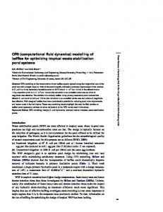
HP

IP

LP

(a) Full Model

(b) HP turbine stub cavity

(c) Mesh around HP rotor trailing edge

Figure 2. Whole turbine steady, main gas path RANS model.

So called “whole engine models” have been used for some time in structural and thermo-mechanical modelling. Examples have been given by Dixon [20], Dixon et al. [21] and Benito et al. [22]. Dixon and Dixon et al. discus thermo-mechanical modelling in some detail. The whole engine thermo-mechanical model shown by Dixon et al. is reproduced in figure 1. As described by Dixon, such finite element analyses (FEA) often assume axisymmetry with approximate treatment of 3D features. Transient analyses are conducted to obtain component temperatures, movements and stresses through a flight cycle. Dixon stated that the main advantage of the whole engine model was its ability to generate its own “boundary conditions” for the downsteam components. For example, cooling air temperatures in the turbine would depend on heat transfer in the internal air system in the compressor. It was also noted that such models contained around 1000 “boundaries” for which aerothermal boundary conditions were required throughout the flight cycle. Dixon et al. confirmed that CFD was a practical tool for determining convective heat transfer in many situations and showed a fully coupled CFD/FEA simulation. Benito et al. presented a detailed 3D solid model of compressor casings and other engine structures. This was used in conjunction with an axisymmetric rotor model to calculate blade tip running clearances. These authors also included comparison with a simplified whole engine model using shell and beam elements which included the engine and its attachment to the test bed. Whereas thermo-mechanical modellers need to consider a transient flight cycle to capture the relatively slow response of component temperatures to changes in operating conditions, aerodynamic design usually considers discrete, steady engine operating conditions. If the gas path flow is also assumed steady (which requires some circumferential or time averaging of the flow as it passes from one blade row to 5

Paper prepared for the 50th Anniversary special edition Part 2 of the Journal of Mechanical Engineering Science, 2009. another) then full main gas path 3D RANS CFD solutions are currently feasible, as discussed in the introduction. Figure 2 shows an example of a steady RANS whole turbine model, as described by Hills [13]. This model has about 22 million mesh nodes and could be run on the 1024 processor HPCx machine in around 1 hour. The geometry definition includes some representation of the turbine hub cavities (seen in figure 2b) to allow the addition of coolant flow to the mainstream, but film cooling injection is modelled as an averaged mass and momentum injection rather than through full resolution of the cooling holes. Improvements on this level of modelling might come from extending the model to include the full main gas path, inclusion of secondary air system flows, extension to unsteady flow so avoiding the averaging of solutions between blade rows, more detailed geometry definition, and coupling to thermo-mechanical models to give more accurate estimates of running geometry.

Figure 3. Mesh for unsteady calculations on an 8.5 stage compressor, Wu et al. (2005). Detailed analysis of engine structural dynamics and aero-mechanical vibration is usually conducted at discrete steady engine operating points, although these points will be chosen to represent an appropriate range of conditions in the flight cycle. As for thermo-mechanical analysis, various FEA structural models are employed, including “whole engine models”. Aero-elastic models using CFD to calculate the air flow and structural vibration modes calculated from FEA have also been in use for some time. An example of a large scale application is given by Wu et al. [23], who reported an unsteady CFD solution for an 8.5 stage compressor. The mesh for this calculation had a total of about 68 million mesh points with 40000 to 75000 mesh points per blade passage. This compares to >106 mesh points per passage in Hills’ aerodynamic model described above. Wu et al.’s model did allow for overtip blade flow leakage, but gaps between the rotors and stators and associated leakage flows were not included. Vibration of the first stage rotor and stator blades was modelled using a modal structural model (rather than direct coupling with FEA) and the simulation was run for about 10 blade vibration cycles (~0.03s in this case), which is longer than might have been needed for the flow to stabilize for fixed blades. To achieve this length of simulation the time-step was varied, being alternately smoothly increased and decreased. This procedure and the relatively coarse mesh resolution may have affected accuracy, although the calculation (which was conducted a few

6

Paper prepared for the 50th Anniversary special edition Part 2 of the Journal of Mechanical Engineering Science, 2009. years ago) clearly illustrates the potential for such large scale analysis. It should also be noted that relatively coarse mesh models involving more components can capture interaction effects that other models miss completely. Such effects have previously been found important in engine vibrations and are often not well understood. An example of this was given by Chew et al. [24] who demonstrated coupling of fan blade flutter in low engine order modes with intake acoustics. As mentioned above, different time-scales emerge as important, depending on the different aspects of engine design to be considered. The largest timescales that will be considered here are on the scale of an engine flight cycle. A typical cycle might last several hours, although substantial periods of this may be at steady running conditions. Thermal response times of components may be of the order of tens of minutes (say ~103s), and these may affect running clearances at all conditions through the degree of incursion into abradable surfaces. Timescales for gas flows and structural vibrations to stabilise at a given operating point are generally much shorter, with steady running conditions expected within a few revolutions of the lowest speed shaft. This could be, for example, of the order of 10-1 seconds. Note, also, that allowing the virtual engine model to adjust shaft speeds, so that the overall shaft power balances are satisfied, might affect the time required for solutions to stabilise. An unsteady CFD solution would have to resolve blade passing events for the highest speed shaft which could have a period of order 10-4s, requiring computational time steps of order 10-6s. It is immediately clear that different modelling approximations may be appropriate for thermo-mechanical modelling than for single operating point aerodynamic, acoustic and vibration investigations. Reduced CFD mesh resolution may be justified in applications where it is more important to capture component interaction than local flow details, but such models will not be suitable for all purposes. However, there is considerable similarity in the modelling methods used for the various applications, and so commonality of software systems can be envisaged. It is assumed here that CFD for the main gas path and secondary air system will be the most computationally intensive element of virtual engine modelling, but it is recognised that coupling with solid models and other “system elements” such as oil, fuel and control systems will be important. While computing time has been emphasised above, other factors such as ease of model set up, levels of engineers’ time required, and turn-around time for the whole modelling process are clearly important. Apart perhaps from Dawes [9], most workers, to date, appear to adopt an evolutionary approach to virtual engine system development, utilising currently accepted modelling techniques and computer codes for solid modelling, mesh generation and numerical solution. For complex geometries, extraction of acceptable geometry definition from solid models and meshing of the fluid and solid domains can be a major bottleneck in the modelling process. For aeroengines this is compounded by the need to differentiate between static (or cold) geometry and running (or hot) geometry. For example, aerodynamic blade design will require evaluation of running blade geometries, which may be defined in a different format from that used for discs and shafts. Some of these issues are discussed further below. 3. CFD METHODS The large scale CFD modelling required for a virtual engine will, for the foreseeable future, involve compromises between accuracy and cost in terms of both

7

Paper prepared for the 50th Anniversary special edition Part 2 of the Journal of Mechanical Engineering Science, 2009. computing and human resources. These issues are discussed and illustrated in the following subsections. 3.1 Accuracy of CFD models Numerical accuracy In principle, assuming a stable and consistent numerical scheme, accuracy of the solution to a set of differential equations can be ensured by sufficient mesh refinement and rigorous solution of the discretised equations. However, current common practice is to use non-uniform meshes with finer resolution in areas where flow gradients are higher. Unless adaptive meshing is used (which is unusual) this requires prior knowledge of the flow structure and mesh requirements, or mesh dependency testing for each solution. In practice, engineers develop standard meshing and solution techniques through numerical experimentation and comparison with measurements. Such “best practice guidelines” are then applied in a more routine manner in the design process, and should strictly be restricted to similar flow conditions to those for which they are derived. This usually excludes “off-design” conditions such as aerofoil stall or severe flow separation. As the available computing power increases, engineering practice may also change. For example, in the early days of 3D CFD applications, a typical blade passage solution might include 105 mesh points, whereas 106 mesh points might be used today. Numerical errors arise either from discretisation of the model differential equations or lack of accuracy of the numerical solution to the discretised equations. The former is defined by the mesh and the discretisation scheme, while the latter is commonly associated with the level of convergence of iterative solution schemes. The rate and level of iterative convergence depends on mesh qualities such as skewness, orthogonality and expansion ratios, as well as the discretisation and solution schemes. Thus, mesh quality is crucial to CFD solutions, but the different CFD solvers will be sensitive to mesh in different ways. The complex interaction of mesh and numerical schemes makes adaptive meshing difficult. With mesh size limited by computing resource, redistributing points to areas of high discretisation error will affect other mesh qualities. However, adaptive meshing and development of numerical methods for robustness of solution and accuracy are current areas of research which will benefit from advances in computing power, and improvements might be expected. The appropriate level of numerical accuracy depends on the fidelity of the mathematical model and how the results are to be used. For example, modelling of turbulence and transition, approximation of boundary conditions and geometrical simplifications often introduce significant errors or uncertainty, and there may be little point in reducing the numerical errors beyond this level. The choice of mathematical models is also limited by the achievable numerical accuracy and computational requirements. (Otherwise DNS might be the generally preferred modelling option.) Thus it is again clear that model and numerical issues are strongly interrelated. It may also be noted that where CFD models are used with automatic procedures to optimise design, there is a danger that the automatic optimiser will drive the design based on numerical (or modelling) errors, and special attention may be needed here. An example of the numerical errors in URANS solutions for a two stage turbine on a CFD mesh with ~2 million nodes was given by Autef et al. [25]. The

8

Paper prepared for the 50th Anniversary special edition Part 2 of the Journal of Mechanical Engineering Science, 2009. discretisation scheme used did not strictly conserve angular momentum, so the difference between turbine efficiency calculated from the calculated torque and that calculated from the inlet and exit flow conditions represents a measure of numerical error. For the cases considered the difference in these two efficiencies varied between 0.01% and 0.32% with the higher errors corresponding to cases where the solution domain included one of the stator-wells. Such errors could be significant when compared to the small changes associated with some design features, or accumulated over a full engine. For steady RANS models of the same turbine Autef et al. found discrepancies in efficiencies as high as 0.8%. These may be partially due to modelling approximations in averaging the flow on the “mixing planes” between the blade rows. These discrepancies in efficiency calculation are consistent with the levels of numerical error found in mesh dependency tests, and can be taken as a measure of the numerical accuracy typically achieved. For LES, the effects of discretisation are generally more complex. Unless high order schemes are used, numerical effects will contribute to dissipation of the resolved turbulence. Mesh refinement alters both the range of turbulence scales resolved and the numerical dissipation. Hence the numerical scheme and the turbulence model are intrinsically linked. In the limiting case of implicit LES (ILES), where no explicit subgrid scale turbulence dissipation is added, the numerical scheme and mesh define the turbulence model. Current turbomachinery codes generally use relatively low order discretisation schemes. The consideration and development of higher order scheme codes for application with LES and RANS is an ongoing area of research which may improve numerical accuracy or allow reduced mesh sizes in the future. Turbulence modelling While large eddy simulation (LES) is gaining acceptance in the research community and attracting interest in industry, most or all current industrial turbomachinery applications of CFD use the Reynolds-averaged Navier-Stokes equations (RANS) with a model of turbulence. While it is generally accepted that there is no universally valid turbulence model, interest and experimentation in the choice of models continues. In some cases this choice has a significant influence on results. Modelling of laminar/turbulent transition is also a very significant issue, of particular relevance in low pressure turbines. Examples of the sensitivity of CFD solutions to turbulence modelling assumptions are given by Volkov et al. [26]. In one example the pressure loss coefficient for flow through a turbine vane varied from 1.26% to 1.78% for different turbulence models. This may be associated with laminar/turbulent transition, and shows that surface shear stress (and heat transfer) can be subject to considerable uncertainty. In the same study, it was also shown that use of different turbulence models in the disc cavity could give differences in the calculated rim seal flow downstream of the vane of up to 0.4% of mainstream flow. This was associated with variations of vortex strength and hence radial pressure gradient in the disc cavity. Comparing these results to the numerical sensitivities discussed above, it may be concluded that inaccuracies in RANS turbulence models are typically of similar magnitude or larger than numerical inaccuracies. For conditions involving separation, such as compressor stall, sensitivity to both turbulence model and mesh refinement is likely to be increased.

9

Paper prepared for the 50th Anniversary special edition Part 2 of the Journal of Mechanical Engineering Science, 2009. In the internal air system it is known that some buoyancy-affected flows (in the centripetal force field) are not well predicted by current URANS models. Such flows commonly occur in compressor disc cavities, such as can be seen in figure 1, and may involve a central, axial flow of coolant air through the rotating cavity with no net radial flow. Figure 4 shows results from 120o sector URANS and LES models for a model compressor disc cavity, as reported by Sun et al. [27]. Both models show large scale unsteady flow features (as have been observed experimentally) but the LES results exhibit a finer flow structure than the RANS solution. The LES model achieved significantly better agreement with velocity and heat transfer measurements than the RANS model. Sun et al. concluded that LES has shown promise for such flows but requires more study and is currently limited by high computational demands. In related studies, 2D steady CFD-based modelling has been developed for such flow situations [28]. This is illustrated in figure 5 which indicates a region of enhanced mixing that accounts for the unsteady flow features not captured by the steady model. In this model the shroud heat transfer is calculated from an empirical correlation. The model reverts to a conventional RANS calculation in the absence of destabilising buoyancy effects. The aim of this research is to improve modelling in design calculations within a thermal modelling environment where use of CFD will be routine.

Figure 4. Instantaneous radial velocity contours on the mid axial plane for buoyancy-affected flow in a rotating cavity [27].

As illustrated by Boudet et al. [29, 30], turbine rim seal flows (in common with compressor disc cavities) can exhibit inherent large scale unsteadiness. It has yet to be established if URANS models can accurately predict hot gas ingestion through the rim seals that can severely affect disc heat transfer. An example, from RANS calculations of flow through a simple axial clearance rim seal is shown in figure 6. The main annulus stator and rotor hubs are shown in perspective from the top, and the arrow represents the main flow direction in the annulus. Contours show concentration of a tracer gas mixed with the cavity inlet flow. No asymmetry is enforced, but the flow is found to be intrinsically three dimensional and unsteady.

10


Shroud Heat Flux – Nat.Conv.Horiz.Plate Correl., Nu = 0.14 Ra0.333 Chara. L= gap/2 ∆T= TW – T

Region of Enhanced Mixing n Fn (A Ra ) with A Region of Enhanced = 1300 n = 0.1 Mixing Ral = fn (dρ/dr)

Stability criteria [Mn2 - r/? (dρ/dr)] > 0 Chara. L= rl -RShaft

2

then

?(d /dr)] ? 0 l

Conventional CFD k-ε Model with 2-layer near wall model

Mass Flow Inlet

Pressure Outlet

Figure 5. Modelling assumptions and calculated streamlines for axisymmetric, steady CFD modelling of buoyancy-affected flow in rotating cavities [28].

Figure 6. Instantaneous computed tracer gas concentration on the annulus hub for a low annulus mass flow, showing inherent 3D nature of rim seal flow [30]. Other examples where RANS turbulence models are of questionable accuracy include film cooling and flow in complex internal blade cooling passages. Resolution of these cooling features also increases mesh size very significantly above requirements for uncooled blade passages. Nevertheless, RANS calculations are increasingly used in cooling studies and often provide useful estimates of heat transfer in complex flows. Empirically based modelling techniques are available for film and internal cooling and can be embedded in CFD-based methods as discussed, for example, by Chew et al [31]. Such methods could be useful in the context of a virtual engine, depending on whether RANS models are considered sufficiently accurate and efficient.

11

Paper prepared for the 50th Anniversary special edition Part 2 of the Journal of Mechanical Engineering Science, 2009. Even with LES, significant concerns regarding turbulence modelling accuracy remain. This particularly applies to near-wall and transition effects, and considerable work is needed to establish these methods. Considering also the additional computing requirements of LES, as discussed in the introduction, it can be said that turbulence modelling will continue to be a limiting factor in engine modelling for the foreseeable future. Geometry definition As already noted, an important aspect of thermo-mechanical modelling is the estimation of engine running geometry. For some components, such as fan blades, the change in shape from static to running conditions can significantly affect flow angles and hence performance. Relative movements of rotating and stationary components are also important as these determine blade tip and seal clearances. Where abradable seal liners are used clearances will depend on the running history as well as any selected steady engine running condition. It is important to recognise that that any assumptions or modelling regarding clearances form part of the engine model, and that this can introduce significant uncertainty. Boundary conditions One attraction of whole engine modelling is that inlet conditions for downstream components are calculated within the model, and these components describe exit conditions for upstream components. Engine flight inlet and exit conditions should be straightforward to specify, except perhaps if crosswind or other unusual conditions are to be investigated. However, unless the engine model includes all internal fluid systems and auxiliary functions such as oil flows, air bleeds and power off-takes, some further boundary conditions will be required. As for geometry definition these should be recognised as part of the engine model, introducing additional uncertainty. Current main annulus flow models require assumptions regarding the internal air system flow rates or pressures, temperatures and degree of swirl velocity. These parameters depend on running clearances. The internal flow also has an effect, through disc and shaft windage, on the shaft power balances. Although these effects are relatively small, they should be accounted for when considering other small changes in aerodynamic performance due to secondary air systems. It may also be noted that internal flow system models are currently modelled in design as one dimensional flow networks, with CFD being used to analyse selected parts of the system. These analyses, together with engine temperature measurements when they are available, inform the thermo-mechanical models that can be used to estimate running clearances. Both the attraction and complexity of including the main annulus flow path, the full internal air system and thermo-mechanical modelling in the same calculation are apparent from the above discussions. Coupled modelling of these aspects of the engine is today achieved to some extent through iteration between design groups. More rapid coupling would make unforeseen consequences of design changes less likely and should allow further exploration of design space. In principal, use of high

12

Paper prepared for the 50th Anniversary special edition Part 2 of the Journal of Mechanical Engineering Science, 2009. fidelity CFD for all air flows coupled to FEA component modelling is very attractive. This would eliminate the need for many user-specified boundary conditions, such as the degree of mainstream gas ingestion into a turbine disc cavity, or the heat transfer coefficients in a thermo-mechanical model. However, the degree of accuracy of such a model using currently available CFD tools has not yet been established. Even with this level of modelling it should also be noted that further boundary conditions, such as air flow from the internal air system to the bearing chambers, and thermal boundary conditions for bearings and other components will have to be supplied from supplementary models. Other modelling issues Combustion modelling is an important area. This is not discussed in this paper, but it may be noted that, for a full description, a large number of detailed chemical reaction rates have to be coupled with the flow dynamics and turbulence, often in two-phase flow. Fluid/solid coupling is considered further in section 4 below. Other topics that have been mentioned above but far from fully explored include choice of modelling level, overall model accuracy and validation, and oil system modelling. Overall model accuracy will depend on the accumulation of errors from different parts of the model. For example in a compressor with a pressure ratio 40:1, a 1% uniform overprediction in small stage efficiency would give an underprediction in delivery temperature of order 10K with significant effects for turbine cooling. As shown, for example by Dixon [20] 10K is around the limit of current modelling errors for steady state thermal analyses. An advantage of current practices is that model adjustments can be made to match engine data. While it is hoped that improved modelling would make predictions more reliable, some verification will be required. Use of CFD for oil systems (and combustors) requires consideration of two phase flows, often combined with complex geometries. As shown for example by Gorse et al. [32], Klingsporn [33], Johnson et al. [34], and Chew and Hills [18] considerable progress has been made in understanding oil system flows from recent research, but uptake of CFD methods for predicting such flows can still be considered to be in its infancy. A recent example is given by Sun et al [35] and is illustrated in figure 7. This shows an internal gear box bounded by the high pressure (HP) shaft, intermediate pressure (IP) shaft, and stator. The presence of the radial drive shaft (RDS) and vent pipes are also indicated. In an initial study an axisymmetric, single phase, CFD model was produced giving some insight into the flow mechanisms involved. All 3D features, such as the bearings, gear teeth, holes and protrusions were modelled axisymmetrically (and time averaged) through addition of extra terms in the governing equations. Extension of this modelling approach to include some 3D features and two phase flow is envisaged, but full representation of all geometrical features may not be required, and could be prohibitive computationally.

13


RDS

RHPG

RHPB

Vent pipes

RIPG

RIPB

RIGB

Seal-1

Seal-2 HP shaft

IP shaft

Seal-3

Figure 7. Sectional view of an internal gear box and CFD model features [35].

3.2 Computational and Process Efficiency Benefits of large scale computer modelling must be weighed against costs which will depend heavily on requirements for computing and engineers’ time for pre and post-processing of models. To some extent computing and processing costs can be interchanged with, for example, larger automatically generated meshes requiring more computing time than meshes optimised by a specialist. Current emphasis in computing is on massively parallel computation, while pre and post-processing depend heavily on software design and implementation. These two crucial aspects are discussed in the following paragraphs. Parallelisation Figure 8 illustrates state-of-art parallel performance of a general purpose turbomachinery CFD code [13]. The URANS model in this case represented a turbine stage sector comprising 8 vanes, 14 blades and disc cavity with full geometric detail including bolts, rotating cover plate hooks and inter-blade platform gaps. An unstructured mesh with about 19 million nodes and two sliding planes was used. The figure shows the ideal speed-up in wall-clock time per iteration that could be obtained from increasing the number of processors and the speed-up achieved for this test case in practice. (The speed-up in wall-clock time is relative to a reference computation on 64 processors; this was the smallest number of processors providing sufficient core memory to run the computation.) Excellent parallel scaling of the computation on the HPCx computer is demonstrated up to 1024 processors. Similar scaling has been obtained for other test cases, with about 20000 mesh nodes per computer core being a rough lower limit for near ideal scaling. Initial results on the HECToR computer confirm these levels of performance.

14


Figure 8. Scaling performance for a combined mainstream and internal air system problem [13]

It is of interest to consider what might be achieved on a massively parallel machine, with ~1 million cores, with current processor power. With 20000 mesh nodes per core, a URANS model with ~20 billion mesh nodes could be run efficiently taking ~100s per (implicit) computational time step (based on current experience). For a virtual engine model, a simulation time of several low pressure (LP) shaft revolutions might be required, and the time step might be of order 10-4 times the LP shaft revolution period, having to resolve blade passing events for the faster high pressure (HP) shaft. This gives an estimated computing wall clock time of ~106s or ~10 days per LP shaft revolution simulation time. The above estimates suggest that in addition to parallel computers with hundreds of thousands of cores, some increase in either the compute speed of the cores and/or the number of cores that can be used efficiently is required to satisfy the demands of virtual engine modelling. A review of possible developments in this field is beyond the scope of this paper, but a few observations may be made. High performance computing is currently going through a period of significant change. For around the last five years, while the original statement of Moore’s law (that the number of transistors that can be included on an integrated circuit board will double approximately every two years) has continued to be true, this has no longer been reflected in increases in processor clock speed due to the higher power consumption required. As noted by Emerson et al [10], power and cooling requirements can lead to lifetime running costs in excess of the cost of the system itself. To avoid this “Power Wall”, the computing industry has been increasing performance by designing multicore CPUs, with the aim being to double the number of cores with each new 15

Paper prepared for the 50th Anniversary special edition Part 2 of the Journal of Mechanical Engineering Science, 2009. generation of CPUs. Quad core CPUs are now widely available with eight core CPUs expected by the end of 2009. It may well be that the traditional MPI model of parallel programming (with one MPI process per core) may not be the best way to take advantage of these new architectures and the necessary paradigm shift is discussed in a very influential paper from UC Berkley [36]. This move to multicore chips was carried out much earlier by the computer graphics industry with current graphics cards already having 128 cores. Despite the attractive cost/performance ratio of these chips, little use has been made of them for high performance computing due to the lack of standards and high-level languages for programming them. This situation has begun to improve with the recent release of the OpenCL standard, although this is not yet supported by all vendors. As an example of what may be possible, Brandvik and Pullan [37] implemented an Euler solver on a graphics processing unit (GPU) and reported speed-ups of up to 40 compared to a conventional Intel CPU. It remains to be seen if these impressive speed-ups can be maintained for a cluster of hundreds or thousands of GPUs when the issues of interGPU communication will become important. The programming paradigm shift discussed above seems likely to be necessary here. Field-programmable gate arrays (FPGA) are another emerging technology that may lead to significant advances in CFD capability. An FPGA is a silicon chip containing an array of configurable logic blocks which can be programmed to perform different functions. In recent years, HPC hardware vendors have begun to offer systems that incorporate FPGAs as co-processors. This allows key parts of an application kernel to be carried out in hardware rather than software with the potential to achieve several orders of magnitude speed-up. Again, a lack of standards has led to slow take-up of these kind of system by the HPC and CFD community. However in the last few years, a drive towards standardisation has been led by the OpenFPGA group [38] which is leading to increased research in this area for CFD. For example, the OpenFGPA group recently claimed on its website that GE had used FPGA technology to significantly reduce CPU times for targeted sections of a jet engine CFD model.

Software design The importance and difficulty of software development has been noted by many workers. Sehra [5] described a “plug n’play” environment for engine analysis in which the user could select from various levels of engine component models to make up the virtual engine. Mark [8] noted that developing large scale codes to integrate multi-scale effects for a complete system is a major bottleneck, requiring teams of 10 to 30 professionals for 5 to 10 years. Discussing the engine simulation programme at Stanford University, Alonso [4] observed that they had developed a different way of doing research including “proper” software engineering and development teams. Holmes [6] highlighted the need for rigorous purging of serial bottlenecks in the parallel computing environment, facilities for storage and recovery of huge amounts of data, and post-processing techniques to extract useful engineering results. Particular challenges related to the use of large scale CFD include geometry definition, mesh generation, input and boundary condition definition, data storage, error control and output processing. Most current turbomachinery CFD model

16

Paper prepared for the 50th Anniversary special edition Part 2 of the Journal of Mechanical Engineering Science, 2009. geometries are idealised to some extent. In a multiphysics modelling environment use of a single source of geometry has distinct advantages. This is most likely to be CADD, which raises issues of how to deal with tolerances, gaps between components, and static to running geometry changes at the mesh generation stage. Mesh generation is currently a bottleneck in the CFD process. As illustrated by Hills [13], automation of meshing for real geometries is most easily done using unstructured meshes, but these lead to more computational demands. Improvement of this process is currently receiving considerable attention by CFD software providers and users, although considerable challenges remain in developing robust, efficient methods for large scale modelling with massive parallel computing. Boundary condition definition for CFD could include coupling to other fluid or solid models of varying degrees of complexity. With the “plug n’play” philosophy described by Sehra [5], this would probably involve coupling a number of different codes for fluid and solid modelling. For example, solid modelling could be done in a stand-alone FEA code, internal air systems might be modelled with a 1D network code or with CFD, and combustor modelling might be done in a different CFD code than that used for the compressor and turbine gas path calculations. An alternative approach, offered by some multiphysics software, is to include all modelling within the same computer programme. An example of this is the “conjugate heating” option available in many commercial CFD codes. This allows heat conduction in solid regions of the domain to be calculated at the same time as the flow and heat transfer in the fluid. Data storage, error control and output processing are all areas needing further work. As mentioned above, Hirsch [7] suggested use of uncertainty analysis to mitigate modelling and other risks, and current models are often adjusted to match to engine test data. Considering the limitations of current CFD methods it is expected that careful validation and interpretation of model results will be needed for the foreseeable future. This will require considerable engineering expertise. 4. FLUID/SOLID COUPLING With a few exceptions, current engine modelling uses separate computer programs for the fluid and solid domains, with information exchanged manually through application of boundary conditions. For example, structural FEA models may use pressure loads from CFD models, and CFD-based flutter and forced response calculations may use structural mode shapes and frequencies from FEA. However, with parallel computers available and increasing interest in multiphysics modelling, more holistic approaches are being developed. Recent examples include 1D network models of the internal air systems combined with FEA thermo-mechanical models presented by Muller [39] and Peschiulli et al. [40]. Development of coupled CFD/FEA thermal analysis has been described by Sun et al. [41] and, as this is of particular interest here, is described further below. In the method described by Sun et al. thermal coupling is achieved by an iterative procedure between FEA and CFD calculations, ensuring continuity of temperature and heat flux. The solid FEA model is treated as unsteady for a given flight cycle while, for computational efficiency, steady CFD simulations are employed. This may be justified by considering the different timescales for the

17

Paper prepared for the 50th Anniversary special edition Part 2 of the Journal of Mechanical Engineering Science, 2009. problem, as discussed in section 2. To further enhance computational efficiency a “frozen flow” or “energy equation only” coupling option was also developed, where only the energy equation is solved (for both solid and fluid domains) during the coupling process. This option takes advantage of the weak dependence of many flows on the thermal boundary conditions. An example of a coupled CFD/FEA solution is illustrated in figures 9 to 12. Here a CFD solution of the rear drive cone cavity provides boundary conditions for an FEA model of an HP compressor drum, with other boundary conditions specified following industrial practice in applying heat transfer correlations. The model shown in figure 9 is used to predict metal temperatures throughout the flight cycle shown in figure 10. Two pre-defined CFD models were supplied for this case, corresponding to idle and maximum take-off (MTO) engine conditions. Streamlines from the axisymmetric CFD solution for the MTO case are shown in figure 11. These show a relatively quiescent, rotating central flow core in the cavity with recirculation, driven by the pumping effect of the rotating drive cone, adjacent to the rotating and stationary walls. Typical results from the model are compared with engine test thermocouple data and are shown in figure 12. Here the model results have used the energy equation only option for CFD/FEA coupling and reasonably good agreement has been shown. Similar levels of agreement with test data have been shown for other test cases. CFD domain

0.25

0.2

0.15 0.7

0.75

0.8

0.85

Figure 9. FEA and CFD model domains for a HP compressor drive cone cavity. 1600

Ramp-4 Cond-3

MTO

Ramp-5 Cond-3

Drive Cone Speed Ω (rad/s)

1400 1200

Acceleration Ramp-2 Cond-2

1000

Idle

Ramp-3 Cond-2

800 600 400 200

Ramp-1 Cond-1

0 0

1000

2000

3000

4000

5000

6000

Time (s)

Figure 10. Transient cycle for the HP compressor drive cone thermal model.

18

Paper prepared for the 50th Anniversary special edition Part 2 of the Journal of Mechanical Engineering Science, 2009. Outlet

rd so es r p

ec riv

e on

Stator

Inlet

HP

m co

Outlet

Outlet

Maximum Take-Off (MTO): Stream function contours

Figure 11. Initial adiabatic CFD solution for the HP compressor drive cone cavity.

Normalised Temperature T/Tref

3.0

Measurement Energy eqn Measurement

2.5

m1

2.0

1.5

1.0 3600

3700 3800

3900

4000 4100

4200

4300 4400

4500

Time t (s)

Figure 12. Monitored temperature history at point m1 for the HP compressor drive cone. In the above example, there are distinct advantages in coupling the separate CFD and FEA codes in comparison to currently available multi-physics codes. These include the availability of the specialist convective boundary conditions in the FEA model used where CFD is not applied, and the ability to take advantage of the different timescales for the fluid and solid regions in the numerical modelling. Typically, a coupled thermal model of this type will require hundreds or thousands of updates to the steady CFD solution as modified surface temperatures are supplied from the FEA model. The computation time required for this type of coupled model may therefore be around one or two orders of magnitude greater than for the standalone CFD model. This approach is currently being developed further, including extension to aero-thermo-mechanical modelling, and clearly has potential for virtual engine modelling. At the same time, other approaches which use CFD to define “lower level” heat transfer boundary conditions for use in the thermo-mechanical model are being developed. An example is the influence coefficient method used by Saunders et al [42]. Implementation of these alternative methods in the same software 19

Paper prepared for the 50th Anniversary special edition Part 2 of the Journal of Mechanical Engineering Science, 2009. package allows engineers to select a level of modelling appropriate to their application. 5. CONCLUSIONS It is appropriate here to conclude with a tentative look forward to the next 50 years. It is clear that computer modelling will play an increasing role in aeroengine design, and that computer hardware is a pacing technology. In the past, Moore’s law has given a reasonable estimate of the rate of increase of capability, but this may not apply in the future. Development is currently in a state of flux with industry moving to multi-core processors and significant research will be required to make efficient use of these. Given the current rate of progress in computer hardware developments, direct numerical solution of the Navier-Stokes equations for a whole engine model will remain out of reach for the next 50 years, and fidelity of CFD simulations will remain limited by turbulence model inaccuracies. The desire to improve solution fidelity through use of fully unsteady simulations and improved turbulence models (notably LES) will ensure that modelling choices must balance accuracy and completeness of models against computational cost. Different compromises will be appropriate for different design purposes and so a wide variety of models will continue to be used. Exactly what comprises a CFD-based virtual engine has not been defined, although it is clear that progress is being made in developing multi-component models. The minimum requirement for a virtual engine might be taken to consist of a CFD model of the main gas path plus some model of the internal air system and a thermo-mechanical model of the engine structure giving running geometries and clearances. With steady RANS modelling for the main gas path, a network model for the internal air systems flow, and current whole engine thermo-mechanical models, a virtual engine model could be run on current computers. Steady CFD modelling of the internal air system, coupled with FEA component models could be possible in the next decade. Full unsteady CFD modelling (URANS) for the main gas path could also be possible within the next decade, although this may be limited to selected design points rather than an aero-thermo-mechanical simulation for a flight cycle. Partial unsteady models with a portion of the main gas path treated as unsteady are already feasible. Whether (or when) these models would represent an efficient use of resources in the design process is not clear. For example, much can be done in optimising design at the component level, and this may benefit from quick turnaround of a large number of smaller simulations rather than a full engine model. Thus it is likely to take a further decade or longer for the routine use of large scale engine models to be fully established. Given the timescales, and cost of software systems development it is appropriate that the aeroengine industry and the research community are now considering the opportunities offered by massively parallel computing, and the challenges presented by the virtual engine. A versatile system and user-friendly environment for engine and component modelling, allowing use of different levels of modelling and automating interfaces between the models would encourage exploration and uptake of new capabilities. The quality of systems for large scale computing will increasingly contribute to industrial competitiveness, and these should be able to evolve to exploit increasing computing power.

20


ACKNOWLEDGEMENTS The authors gratefully acknowledge contributions to the work described above, including the supply of some figures, from colleagues at the Thermo-Fluid System University Technology Centre, Rolls-Royce plc and other collaborating institutions. Financial support from Rolls-Royce plc, the Engineering and Physical Sciences Research Council, the Department of Trade and Industry, the European Commission, Alstom Power and the University of Surrey is also gratefully acknowledged. REFERENCES 1. Chew, J.W., 2009. Developments in turbomachinery internal air systems. J. Mechanical Engineering Science, 50th anniversary special issue Part 1. 2. Gorrell, S., 2006. An Air Force research laboratory perspective on high fidelity simulations. ASME Turbo Expo., http://gtsl.ase.uc.edu/IGTI-panel/. 3. Yao, J., Gorreee, S. and Wadia, A., 2007. Unsteady RANS analysis of distortiontransfer through multistage fans. ASME Turbo Expo., http://gtsl.ase.uc.edu/IGTI-panel/. 4. Alonso, J.J., 2006. Stanford University perspective on high-fidelity engine simulation within the DOE ASC program. ASME Turbo Expo., http://gtsl.ase.uc.edu/IGTI-panel/. 5. Sehra, A.K., 2006. The numerical propulsion system simulation: A vision for virtual engine testing. ASME Turbo Expo., http://gtsl.ase.uc.edu/IGTI-panel/. 6. Holmes, G., 2006. Large-scale unsteady CFD for turbomachinery. ASME Turbo Expo., http://gtsl.ase.uc.edu/IGTI-panel/. 7. Hirsch, C., 2006. High-Fidelity (3D&3D time accurate) engine simulation. ASME Turbo Expo., http://gtsl.ase.uc.edu/IGTI-panel/. 8. Mark, A., 2007. Scientific software in a petascale computational environement. ASME Turbo Expo., http://gtsl.ase.uc.edu/IGTI-panel/. 9. Dawes, W.N., 2007. Technical challenges for a real virtual engine. ASME Turbo Expo., http://gtsl.ase.uc.edu/IGTI-panel/. 10. Emerson, D.R., Sunderland, A.J. and Ashworth, M., 2007. High performance computing and computational aerodynamics in the UK. The Aeronautical Journal, UK Applied Aerodynamics Consortium special edition, vol. 111, pp. 125-131. 11. Tucker, P.G., 2007. Introduction. Computational aerodynamics. Phil. Trans.R. Soc. A, Aerospace CFD Theme Issue, vol. 365, pp. 2379-2388. 12. HECToR- UK national supercomputing service, http://www.hector.ac.uk/ 13. Hills, N.J., 2007. Achieving high parallel performance for an unstructured unsteady turbomachinery CFD code. The Aeronautical Journal, UK Applied Aerodynamics Consortium special edition, vol. 111, pp. 185-193. 14. Nayyar, P., Barakos, G.N. and Badcock, K.J., 2007. Numerical study of transonic cavity flows using large-eddy and detached-eddy simulation. The Aeronautical Journal, UK Applied Aerodynamics Consortium special edition, vol. 111, pp. 153164.

21

Paper prepared for the 50th Anniversary special edition Part 2 of the Journal of Mechanical Engineering Science, 2009. 15. Li, Q., Page, G.J. and McGuirk, J.J., 2007 Large-eddy simulation of twin impinging jets in crossflow. The Aeronautical Journal, UK Applied Aerodynamics Consortium special edition, vol. 111, pp. 195-206. 16. Gatski, T.B., Rumsey, C.L. and Manceau, R., 2007. Current trends in modelling research for turbulent aerodynamic flows. Phil. Trans.R. Soc. A, Aerospace CFD Theme Issue, vol. 365, pp. 2389-2418. 17. Secundov, A.N., Birch, S.F. and Tucker, P.G., 2007, Propulsive jets and their acoustics. Phil. Trans.R. Soc. A, Aerospace CFD Theme Issue, vol. 365, pp. 24432467. 18. Chew, J.W. and Hills, N.J., 2007, CFD for Turbomachinery Internal Air Systems. Phil. Trans.R. Soc. A, Aerospace CFD Theme Issue, vol. 365, pp. 2587-2611. 19. Spalart, P.R., 2000. Strategies for turbulence modelling and simulations. Int. J. Heat Fluid Flow, vol. 21, pp. 252-263. 20. Dixon, J.A., 1999. Gas turbine critical component temperature predictions for fatigue life and integrity considerations. ISABE XIV IS/UNK05. 21. Dixon, J.A, Verdicchio, J.A., Benito, D., Karl, A. and Tham, K.M., 2004. Recent developments in gas turbine component temperature prediction methods, using computational fluid dynamics and optimization tools, in conjunction with more conventional finite element analysis techniques. Proc. Instn Mech. Engrs Vol. 218 Part A: J. Power and Energy, pp. 241-155. 22. Benito, D., Dixon, J. and Metherell, P., 2008. 3D thermo-mechanical modelling method to predict compressor local tip running clearances. Proc. ASME Turbo Expo, Berlin, Germany. 23. Wu, X., Vahdati, M., Sayma, A. I.& Imregun, M., 2005. Whole-annulus aeroelasticity analysis of a 17-bladerow WRF compressor using an unstructured Naveir-stokes solver. International Journal of Computational Fluid Dynamics. Vol. 19, pp. 211-223. 24. Chew, J.W., Vahdati, M. and Imregun, M., 1998. Predicted influence of intake acoustics upon part speed fan flutter. ASME paper 98-GT-558. 25. Autef, V.N.D., Chew, J.W., Hills, N.J. and Brunton, I.L., 2007. Turbine statorwell flow modeling. Proc., 8th ISAIF conference, Lyon, July 2007. 26. Volkov, K., Hills, N.J. and Chew, J.W., 2008. Simulation of turbulent flows in turbine disc cavities and blade passages. Paper GT2008-50672, Proc. of ASME Turbo Expo 2008. 27. Sun, Z., Lindblad, K., Chew, J. W. and Young, C., 2007, “LES and RANS Investigations into Buoyancy-affected convection in a rotating cavity with a central axial throughflow”, ASME Trans., Journal of Engineering for Gas Turbines and Power, Volume 129, pp. 318-325. 28. Kilfoil, A.S.R. and Chew, J.W., 2009. Modelling of buoyancy-affected flow in corotating disc cavities. Paper GT2009-59214, Proc. of ASME Turbo Expo 2009. 29. Boudet, J., Hills, N.J. and Chew, J.W., 2006. Numerical simulation of the flow interaction between turbine main annulus and disc cavities. Paper GT2006-90307. ASME Turbo Expo 2006. 30. Boudet, J., Autef, V.N.D., Chew, J.W., Hills, N.J. and Gentilhomme, O., 2005. Numerical simulation of rim seal flows in axial turbines. The Aeronautical Journal, vol. 109, 373- 383. 31. Chew, J.W., Taylor, I.J. and Bonsell, J.J., 1996. CFD developments for turbine blade heat transfer. Third Int. Conf. on Computers in Reciprocating Engines and Gas Turbines, I. Mech. E. Conference Transaction 1996-1.

22

Paper prepared for the 50th Anniversary special edition Part 2 of the Journal of Mechanical Engineering Science, 2009. 32. Gorse, P., Willenborg, K., Busam, S., Ebner, J., Dullenkopf, K. and Wittig, S., 2003. 3D-LDA measurements in an aero-engine bearing chamber. Proc. ASME Turbo Expo, paper GT2003- 38376. 33. Klingsporn, M., 2004. Advanced Transmission and Oil System Concepts for Modern Aero-Engines. Proc. ASME Turbo Expo, paper GT2004-53578. 34. Johnson, G., Chandra, B., Foord, C. and Simmons, K., 2008. Windage Power Losses From Spiral Bevel Gears With Varying Oil Flows and Shroud Configurations. Proc. ASME Turbo Expo, paper GT2008-50424. 35. Sun, Z., Chew, J.W. and Fomison, N., 2009. Numerical simulation of complex flow in an aeroengine gearbox. Proc. of ASME Turbo Expo 2009, paper GT200959530. 36. Asanovic, K et al. The landscape of parallel computing research: a view from Berkley. Tech. Rep. UCB/EECS-2006-183. UC Berkley 2006. 37. Brandvik, T. and Pullan, G., 2007. Acceleration of two-dimensional Euler software using commodity graphics hardware. Proc. IMechE, vol. 221 part C: J. Mech. Eng. Sci., 1745-1748. 38. OpenFPGA Group. www.openfpga.com 39. Muller, Y., 2008. Secondary air system model for integrated thermomechanical analysis of a jet engine. Proc. of ASME Turbo Expo, paper GT2008-50078. 40. Peschiulli, A., Coutandin, D., DelCioppo, M. and Damasio, M., 2009. Development of a numerical procedure for integrated multidisciplinary thermal-fluidstructural analysis of an aeroengine turbine. Proc.of ASME Turbo Expo, paper GT2009-59875.. 41. Sun, Z., Chew, J.W., Hills, N.J., Volkov, K.N. and Barnes, C.J., 2008. Efficient FEA/CFD thermal coupling for engineering applications. Paper GT2008-50638, ASME Turbo Expo 2008. 42. Saunders, K., Alizadeh, S., Lewis, L.V. and Provins, J., 2007. The use of CFD to generate heat transfer boundary conditions for a rotor-stator cavity in a compressor drum thermal model. Paper GT2007-28333, ASME Turbo Expo 2007.

23