7th International Exergy, Energy and Environment Symposium
Slug Catcher Multiphase CFD Modelling: Optimization and with Industrial Standards 1*
1
Gianluca MONTENEGRO, 1 Gianluca D’ERRICO, 1 Augusto DELLA TORRE, 2 Luca CADEI, 2 Silvia MASI
Politecnico di Milano, Department of Energy, Internal Combustion Engines Group, via Lambruschini, Milano, I-20156, Italy 2 ENI S.P.A. Via Emilia, 1 Piazza Ezio Vanoni 1,20097 San Donato Milanese (MI) - Italy * E-mail:
[email protected]
Keywords: Slug catcher, multiphase, OpenFOAM, CFD Abstract In the oil & gas industry, the traditional procedure for slug catcher design is based on the Stokes' law. Design equations are obtained from a 1-D analysis and validated with experimental data. Therefore, this method basically relies on simplified models and empirical correlations. For this reason, an over margin factor from 20 to 40% is usually applied. In this paper, a simplified CFD procedure for the modeling of the gas-liquid separation is presented. Steady state and transient models have been considered for single phase and multiphase fluids, using OpenFOAM. The influence of flow model and mesh grid on results have been evaluated as a trade-off between solution accuracy and computational efforts, in order to assess the applicability of these models to industry. A comparison of the industrial validation procedure with the CFD analysis has been realized, focusing on the pros and cons of the two different approaches. A new application solver has been constructed and programmed in order to get the most accurate results with the minimum computational efforts. This solver is based on a completely new and innovative approach to the Navier-Stokes equations for multiphase flow. New model proposed has been used for the evaluation of design for the two slug catchers studied, in order to get a better separation and fluids management. I. Introduction
industry for the design and validation procedure of the slug catcher facility. The numerical calculation are carried out using the OpenFOAM® code (OpenFOAM documentation), an advanced and free CFD Toolbox, able to customize and extend software solutions to the simulations process across a wide range of physical phenomena and at different level of in-depth analysis. OpenFOAM has an extensive range of features to solve any continuum mechanics problem, ranging from complex fluid flows involving chemical reactions, turbulence and heat transfer, to solid dynamics and electromagnetics. It is written in a highly efficient C++ object oriented programming, and, since it is open source, it is easily customizable. For this reason it has been adopted for this industrial project as it allows to develop solvers ad hoc for a physical problem.
The global energy demand has grown exponentially since the last century, and according to the main energy agencies an increase of 41% is expected in 2035. In this context, the fossil fuels, and in particular the oil and the natural gas, will maintain their primary role, achieving the 75% of the market share (BP, 2014). The inexorably depletion of the traditional and easily exploitable reservoir has led the major Oil Company to focus their attention on the improvement of production efficiencies. One of the main challenges in the optimizations process of the production systems is the development of innovative and precise methodologies able to handle the multiphase flow, which is a very common phenomenon in the actual Oil & Gas applications and can cause the onset of critical working conditions in upstream and downstream apparatus. This last characteristic leads inexorably to the loss of production capacity of the entire production system, composed by the reservoir, the well and the surface facilities, and finally to the decrease of the company profit. In the current work, a CFD analysis is used to study the first stage of the separation process between gas and oil occurring at the slug catcher facility, considering also the capacity of the slug catcher to handle and distribute the multiphase flow coming from the wellhead. The Oil & Gas world has usually preferred to exploit experimental data or simplified approach to design and validate the parts of the slug catcher facility responsible for the separation of the phases and for the management of the incoming flow. The project starts from the analysis of the main current standard methodologies adopted in the petroleum
Nomenclature g p V U d L t
: Gravitational constant (m.s-2) : Pressure (N.m-2) : Volume (m3) : Velocity (m.s-1) : Diameter (m) : Length (m) : Time (s)
Greek letters α : Volume phase fraction (-) : Density (kg.m-3) ρ : Viscosity (Pa.s) µ
-1-
7th International Exergy, Energy and Environment Symposium
II. The slug catcher
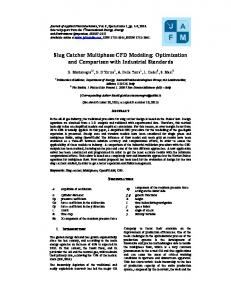
offshore application thanks to its particular geometry. The main disadvantage of this device is the dependence on strict operational conditions that reduces flexibility. The configuration analysed in this work is the finger type one, which is represented in Fig. 1. However the CFD methodologies developed in the project are also applicable in case of different geometry maintaining the right level of accuracy.
The slug catcher is stationary equipment used in the upstream oil production system. The main functions of a slug catcher can be summarized as follows: • It provides a buffer and storage volume for the fluids coming from the well; • It maintains constant and close to the optimum the operating condition of the upstream and downstream facility, allowing to maximize the oil production. This function permits also to ensure a constant flow rate to the gas line and to the oil treating section; • It manages the intermittent slug flow generated in the upstream section of the production facility, distributing homogeneously the incoming flux; • it provides a first stage of separation between the gas and the liquid phases.
III. The multi phase flow pattern The multiphase flow coming from the well, is composed mainly by gas and liquid. The flow inside the horizontal pipes of the slug catcher can be classified considering the distribution of the different phases inside the geometry that defines the flow regime (Figure 2). The distribution assumed by the different phases inside the pipes and the devices is an important parameter in the study of the multiphase flow behavior. The specific distributions are usually divided into flow regimes model, with particular features and characteristics, for vertical or horizontal pipes. Here, the attention is focused on the last ones (Ergun, 1952). • The bubble flow: the small gas bubbles are dispersed into the continuous liquid phase. It is typical for high volumetric flow rate. • The stratified flow: generated by the very low velocity of both phases, which leads to a complete separation of the mixture. The liquid is separated by an undisturbed interface from the gas. • The stratified-wavy flow: as the gas velocity increases, small waves in the flux direction are generated. The dimension of the waves depends on the relative velocity between the phases. The waves do not reach the upper part of the pipe. • The intermittent flow: the continuously increase of the gas velocity conducts the small waves to reach the top of the pipe. This regime is characterized by the presence of big waves alternated to small waves. This regime can be divided into two sub-category: -the plug flow: this regime is characterized by big elongated bubbles of gas, which do not reach the dimension of the full section of the pipe. Thus, a liquid volume is always presents in the bottom part of the pipe. -the slug flow: when the gas velocity increases another time, the bubbles achieve a dimension comparable with the pipe diameter. Hence, the flow inside the pipe is characterized by an alternation between the gas and the liquid phase. • The annular flow: increasing the gas volumetric flow rate, the liquid is pushed on the pipe wall, forming an annular film, thicker on the bottom of the duct. The interface is characterized by small waves and small droplets coming from the liquid film. • The mist flow: for very high gas velocity, the liquid is transported in the flux in small droplets dispersed in the gas continuous phase. The flow is considered completely dispersed in this
Fig. 1: Flow regimes in horizontal pipes
According to their geometrical characteristics, they can be classified in three main categories (Engineering data book, 2004): • Vessel type: simple two phase separation vessel. The vessel needs to be large enough to handle large liquid slugs and a high design pressure. The configuration of this device is suitable for limited offshore/onshore plot size in the field. The main disadvantage of this type of slug catcher is the reduced buffer storage volume, generally less than 100 m3. • Multi-pipe type (also called finger-type): in this case the pipeline from the well is directly connected to a manifold that collects and distributes the flow to several tubes. This configuration offers a technical-economical advantage both to manage the level of pressure and to realize a buffer storage volume, ensuring a continuous flow to the downstream facility. Moreover, the finger type configuration gives to the operator larger layout flexibility along with the capacity to handle large slug flow from the well. However, a large number of pipes is required to provide sufficient volume and this results in a wide slug catcher footprint. • Parking loop type: this hybrid configuration joins the features of the vessel and those of the finger type slug catchers. This slug catcher type is adopted to manage liquid carry over in counter current gas/liquid flow. It is also suitable for the
-2-
7th International Exergy, Energy and Environment Symposium
and drag forces acting on the particles. The particles segregation starts from the top of the pipe suddenly at the terminal velocity.
work, taking into account the worst condition for the separation process allowed inside the facility, and it is composed by two phases: natural gas (continuous phase) and raw oil (dispersed phase, small droplets).
4gddroplet ρl − ρ g Vt = 3Cd ρ g
(1)
The drag model can be chosen from a variety of different experimental or semi-empirical relations. In this work the Schiller Neumann formulation is considered [5]:
24 1+ 0.15 Re 0.687 ( p ) Cd = Re p 0.44
( for Re
p
≤1000 )
( for Re
p
> 1000)
(2)
Where the Reynolds number depends on the relative velocity between the gas and the liquid phases:
Fig. 2: Flow regimes in horizontal pipes
The first step needed to proceed with a CFD analysis of the multiphase flow inside a slug catcher is the study of the actual design procedure for finger type slug catcher already used in the industrial practice. It is based on simple concepts of fluid dynamics and on the experience in engineering these devices. The technical sizing procedure currently adopted for a finger type slug catcher consists of the following main steps: 1) Storage volume calculation; 2) Selection of number and diameter of fingers; 3) Sizing of fingers; 4) Sizing of inlet header; 5) Sizing of downcomer; 6) Sizing of riser; 7) Sizing of outlet header and equalization lines. This procedure involves an iterative process that is composed of series of steps based on the selection of the number and diameter of the fingers, followed by the validation of this selection. If the selection made are shown to be inadequate, the procedure is repeated starting from the second point of the previous list, varying the number of the fingers, and/or the diameter. Once the design is successfully completed, the overall dimensions are evaluated in order to check the compatibility of these parameters with the plant layout and pipe-rack. It is important to focus the attention on the relationship implemented in this procedure to compute the length of separation. In fact, some experimental equations depending on the geometry of the slug catcher device and on the composition of oil and gas are derived and interpolated from graph that shows the separation length as a function of the superficial velocity and the density of the gas (as depicted in Figure 3). In this project an alternative industrial approach to the design of the slug catcher separation mechanism is briefly introduced. This procedure will be used for quick comparisons with the CFD solutions. This procedure is based on the one-dimensional application of the Stoke’s law. The particle segregation is modelled with a constant terminal velocity that produces a flux of liquid towards the bottom of the geometry. The terminal velocity is computed rearranging the balance between gravity, buoyancy
Re p =
ρl ddroplet Ur µl
(3)
Fig. 3: 1D Stokes approach
The industrial standards introduced above, implies the utilization of several simplifying assumptions. Thus, many theoretical problems arise from these procedures, generating some sources of errors, which can affect the final results. These problems are briefly listed below IV. The two phase approach Usually the dynamics of two-phase flow is modelled using the Navier-Stokes equations for a Newtonian fluid. The main approaches to the simulation of this kind of phenomena are (Weller, 2002; Hill, 1998; Gossman et al., 1992; Rusche, 2002): • Direct Numerical Simulation (DNS): the NavierStokes equations are employed without further manipulation. The topology of the interface between the phases is determined as a part of the solution. • Dispersed Phase Element (DPE): this model is also referred to as the Euler-Lagrangian approach. The equations of motion for the dispersed phase is expressed in the Lagrangian formulation, while the conservation equations for the continuous phase are expressed in the Eulerian frame. • Two-Fluid Model: in this case both phases are characterized using the Eulerian conservation equations. Hence the model is also referred to as the Euler-Euler frame. The Two-Fluid model has been adopted in this work in order to simulate the two-phase dynamic. This methodology requires less computational efforts than the DNS and it is more suitable for every flow regime than the DPE, thanks to the two-way coupling granted by the Euler-Euler approach. -3-
7th International Exergy, Energy and Environment Symposium
The governing equations are written in the averaged form for both the fluids, considering each phase as continuous, allowing in this way the interpenetration of one phase into the other one. The momentum transfer between the two different phases is taken into account through the term M ϕ which considers the forces acting
equation, reducing in this way the equations to be solved to simulate the multiphase phenomenon. Instead of solving the continuity equation and two momentum transfer equations, one for each phases, thus three equations. The simplified approach presented here allows to solve only one continuity equation and one momentum transfer equation for the continuous phase. The continuity equation introduced, simulates the dispersed phase flow and the separation process between the liquid and the gas. Applying the steady state condition and the hypothesis of incompressible flow, the mass conservation equation is rearranged in the following form, which is implemented in the solver code (Malalasekera, 2007; Ferziger):
on the interface between the fluids: drag, lift, virtual mass and turbulent effect. For each phase it is possible to express the mass and momentum conservation respectively as [10]:
∂α ϕ (4) + ∇ (αϕ Uϕ ) = 0 ∂t M ∂αϕ Uϕ α + ∇ (αϕ Uϕ Uϕ ) + ∇ (αϕ Rϕeff) = − ϕ ∇p+ αϕ g+ ϕ (5) ∂t ρϕ ρϕ
∂ρ + ∇ ⋅ ( ρU ) = 0 ∂t
eff
Where R is the combined turbulent and viscous stress Reynolds number, M ϕ is the averaged inter-
(9) The general form of the momentum conservation equation, obtained with the Eulerian approach fixing a cell volume in the space, can be written with the following notation:
phase momentum transfer term. For clarity sake, it is reported the volume phase fraction αϕ , defined as:
αa =
Vαa Vα a +Vα b
∂ρU + ∇ ⋅ ( ρUU ) = ∇ ⋅ ( T ) + Sf ∂t (10) where T is the stress tensor of a Newtonian fluid.
(6)
Combining the two continuity equations for the two phases ϕ = a and ϕ = b it is possible to formulate the volumetric continuity equation as: ∇ ⋅U = 0 (7) Where,
Applying the steady state and incompressible flow condition and neglecting the diffusive transport of the liquid particles, which are transported only by convection, the final equation for the transport of the droplet volume fraction can be formulated as follows:
U = α aUa + α bUb .
The set of equations is rearranged into a pressure equation and then solved. In particular, for what concern the calculation of the interphase momentum, its value id determined by different contributions. In our specific case, due to the limited size of the droplets considered lift is neglected and only drag and turbulent drag are modelled.
M αV
α
= Fd + Ftd
∂α + ∇ ⋅ (αU ) = Sp ∂t (11) The source term Sp , is mathematically introduced as
a scalar quantity inside this formulation and should mimic the separation of the liquid phase due to the gravity effect. Considering the physics of the sedimentation process, it is possible to understand that the gravity produces a flow of liquid particles in the direction of the gravity. This flow produces a flux that can be conveniently represented by the divergence operator. For this reason, it is possible to rearrange the source term as a flux term, given by a vertical velocity multiplied by the orthogonal area of the cells:
(8)
The turbulence (Gossman, 1992) is introduced as a standard k-ε model, which is suitable for the particular flow conditions under study, including source terms to incorporate the dispersed phase on turbulence. This approach can provide the best approximation of a real two-phase physical phenomenon. The main drawback is the computational burden required to perform the simulation, mainly due to the intrinsic unsteady nature of the model.
∂α + ∇ ⋅ (αU ) = ∇ ⋅ (αVt ) . ∂t
(12)
The volumetric flux of this new divergence term comes from the terminal velocity calculated in Eq.1. The face center value of the terminal velocity used in the discretization of the divergence term is obtained by linear interpolation of the cell center value of the terminal velocity field. Equation 12 can be also written in a more compact formulation considering the volumetric flux given by the sum of the two convective contributions: gas convection and deposition:
V. Simplified single phase approach To overcome the high demand of computation resources when the simulation of a real geometry is addressed, an innovative model, based on a singlephase approach has been developed, is proposed. The Navier-Stokes equation is solved only for the continuous phase, the gaseous phase considered as incompressible, and the segregation process of the liquid droplet is modelled with the transport of the scalar variable α, which represents the volumetric fraction of liquid in the total fluid flow. The idea is to represent the effect of the dispersed phase with the help of a simple scalar transport
∂α + ∇ ⋅ α (U - Vt ) = 0 ∂t
(13)
In this framework, it is really important to define the correct boundary on the terminal velocity. As a Matter of fact, imposing at the boundary a Neumann -4-
7th International Exergy, Energy and Environment Symposium
condition would imply to assign an incoming and outgoing flux at those patches where there should not be any kind of flow. To accommodate this issue a slip type boundary condition on the terminal velocity field has been imposed. The drag coefficient is computed with the SchillerNeumann model previously presented. In this case, since there is only one velocity (the gas velocity), assumptions need to be made in order to estimate the relative velocities. In particular, it has been assumed that the two phases are moving one with respect to the other only by the term responsible for the settling Vt . The value of
Vt
therefore, the CFD results are compared to the 1D Stokes’ approach. The particle diameter used for the calculations has been chosen equal to 150 µm.
Fig. 5: Single-phase approach.
is, therefore, determined by means of
an iterative procedure. An advantage of this simplified approach is that the system of equations is now decoupled. There in no more interaction between the momentum and continuity equations of the two phases, but there is a single phase system of equation plus a decoupled transport equation which exploits the convective term. This means that the system can be modelled also as a steady state process, resulting in a dramatic reduction of the computation demand.
Fig. 6: Two-phases approach.
The 1D Stokes’ method underestimates the segregation length, providing a value of 9.68 m. The maximum error obtained is about 40%. The main reason of this discrepancy is due to the fact that the 1D theory approximates the flow as a 1D flow, whose component of the velocity in the axis direction is uniformly distributed over the flow area. This is obviously not realistic and therefore does not account that in the middle on the pipe the velocity is higher, causing an increase of the length necessary to allow the separation. Imposing uniform distribution of the velocity and setting slip boundary conditions, the case becomes equivalent to a 1D case, resulting in a separation length close to one given by the 1D theory. After having validated the two approaches, a simple part of a real slug catcher, composed of a finger and a 45° inclined downcomer has been considered (Fig. 7). This geometry permits to test the behaviour of CFD solvers, comparing the results obtained with the experimental industrial standards. The downcomer is 4 m long, with a diameter of 30 inches. The finger is inclined by 1.15°, and is 40 m long, with a diameter of 48 inches. The mesh size has been chosen after a sensitivity analysis on the volumetric fraction distribution. The calculation grid, considering these two parameters, has been generated using the mesh cartesian mesh generator of OpenFOAM, namely snappyHexMesh. This mesh generator creates a high quality, hex-dominant mesh starting from a background mesh and a surface representation of the geometry that will be studied. Furthermore, surface refinement and boundary layers have been included in the final mesh. Also in this case several test simulations are performed, in order to further optimize both the CFD solvers. The attention has been posed on the influence of the mesh and the boundary condition characteristics.
VI. Preliminary simulations To validate the simplified approach, simulations were carried out on a pipe with squared section. This allowed to have a calculation mesh free from typical issues that generate errors in order to quickly optimize the CFD application. The geometry is represented by a 16 meters pipe, with a squared cross section cross section of 0.36 m2 (Fig. 4). In this way it is possible to simplify the calculations, reducing the time necessary to solve the problem, and providing the possibility to easily analyse the results. The mesh in this case is composed by a simple block.
Fig. 4: Square duct geometry and mesh detail.
The simulations are managed focusing the attention on the influence on the final solution of different parameters, such as the mesh size, the discretization schemes and the solution algorithms. The results obtained have allowed the comparison of both the CFD approaches: the eulerian-eulerian two phase approach and the simplified single-phase one. The simulated cases are illustrated in the Figures 5 and 6, where a threshold filter highlights a separation efficiency of 99%. It can be noticed that the length of the complete segregation of the liquid phase is approximately the same for the two approaches, approximately 14 m. In this particular case there is no experimental correlation that can be exploited, -5-
7th International Exergy, Energy and Environment Symposium
droplets start to aggregate, generating particles with larger diameter. The model implemented individuates the αlim value when a cell is completely full of spherical particles without merging phenomena (Fig. 10).
Fig. 7: Downcomer + finger geometry and final mesh detail.
The final results are shown in Fig. 8. As it is possible to see, in this case the results obtained, in terms of liquid volumetric fraction, using the single-phase approximation are not in agreement with the eulerianeulerian approach. In particular, it seems to overestimate the total length of separation, whereas the two-phase simulation computes a separation in agreement with the industrial experimental database.
Fig. 10: α limit condition.
The model maintains constant the value of the droplet diameter until the alpha limit is reached. After this point, the particle diameter is obtained with an exponential trendline, which interpolates the initial diameter of the liquid sphere and the maximum diameter achievable, or in other words the cell equivalent length. The result obtained using the modified single-phase solver similar to the one achieved with the two-phase solver (Fig. 11). This confirms the improvement in the prediction that can be achieved introducing the coalescence model. However, the result is conditioned by the assumption made to define the limit level of α and to interpolate the values of the maximum diameter.
Fig. 8: a) Single-phase threshold filter; b) Two-phase threshold filter.
An analysis of the velocity vector in the direction orthogonal to the main flux revealed the presence of a lifting effect at the end of the downcomer, where the rotational flow caused by the variation of the geometry disturbs the deposition process. The liquid droplets, modelled as spherical particles, are lifted by this flow causing the overestimation of the separation length. This effect is shown in Fig. 9. Fig. 11: a) Single-phase coalescence model threshold filter; b) Two-phase threshold filter.
The final comparison with the industrial standards illustrates a substantial underestimation of the experimental procedure and of the 1D Stokes’ approach compared to the CFD analysis (Tab. 1). This comparison reveals the lack of accuracy achieved with the main typical process design adopted in the industry which do not take into account 3D effects. Tab. 1: Comparison of the different approaches. Experimental 1D Stokes CFD approach approach Lsep[m] 10.06 11.29 13.00
Fig. 9: Rotational flow inside the finger.
The solver does not take into account that the liquid deposited on the bottom of the pipe cannot be dragged in the same way of single droplets. For this reason, a coalescence model has been implemented to simulate the real behaviour of the liquid already collected at the bottom of the geometry, limiting this lifting effect. The idea in this case is to find a threshold value of the volume fraction of liquid, above which the
Moreover, it is important to highlight that the reduction of time achieved using the new single-phase approach to the study of the multiphase flow dynamics, is around the 25
-6-
7th International Exergy, Energy and Environment Symposium
VII. Real case simulations Every simulation presented in the previous section is performed with simplified. In this section, the facility considered is a real finger type slug catcher (Fig. 12).
Fig. 14: Gas flow distribution.
The figure shows an acceptable level of symmetry in the fluid distribution, which can be observed in the velocity field obtained inside the pipes. In order to have a clearer understanding on the flow distribution, the volumetric flow have been probed across general planes defined by the user allowing to evaluate how the flow is distributed along the fingers. This is an important information since the usual procedure is to assume a uniform distribution of the gas flow over all the fingers.
Fig. 12: a) Slug catcher finger-type 3D model.
The 3D model can be simplified exploiting the symmetry of the device. The final 3D model used is reported in Fig. 13. The mesh is generated considering the results of the previous preliminary simulations, and in particular the downcomer plus finger configuration.
Tab. 2: Percentage of the total flows in the different pipes. Q [%] Splitter 1 51.16% Splitter 2 48.84% Downcomer 1 14.76% Downcomer 2 15.10% Downcomer 3 20.12% Downcomer 4 20.14% Downcomer 5 15.11% Downcomer 6 14.77%
As it is possible to see (Tab. 2), the current layout of the slug catcher seems to gather and distribute homogenously the incoming flow from the well. Having evaluated the fluid dynamics of the device, it is now possible to proceed with the multi-phase simulation using the single phase approximated solver (Fig. 15) and the multiphase approach (Fig. 16). The average particle diameter is set to 1000 µm, in agreement with the specifications of the extraction site.
Fig. 13: Simplified 3D model.
A single phase simulation of the slug catcher has been performed to assess the capacity of the facility to receive and to distribute homogeneously the incoming flow. For this purpose a single phase solver, whitout considering the scalar transport equation of the volumetric fraction, have been used. The flow is assumed to be completely composed by gas. The solver used for this simulation is already implemented in OpenFOAM, for incompressible flow and exploits the SIMPLE algorithm for steady state problems. The simulation is performed considering a turbulent incompressible flow and a steady state conditions. The result is shown in Fig. 14.
Fig. 15: Single phase simulation.
-7-
7th International Exergy, Energy and Environment Symposium
the high level of accuracy typical of the two-phase application. In this way the perfect trade-off, between accuracy and reduction of required simulation time, is reached, making economically and technically feasible the application of the CFD approach in the Oil&Gas sector. The procedure (Fig. 17) is an iterative process that starts from the current experimental industrial standard and consequently applies the CFD tools presented previously in the report. The single-phase steady state approach is used to obtain a quick and accurate distribution of the phases inside the slug catcher. The results obtained in this way are then used as initial condition for the two-phase unsteady application, reducing the time required for the simulation.
Fig. 16: Two phases simulation.
The assumption of incompressible flow approximates the real flow characteristics, but considering that the pressure drop along a slug catcher is limited, the expansion ratio is approximately equal, to one. This allows to neglect the compressibility without losing solution accuracy. Moreover, the flow velocities inside the pipes correspond to low Mach numbers (