Dec 12, 2003 - ABSTRACT. Metals extraction using heap-leaching methods is very slow particularly for sulphide ores, but the pathway to faster leaching is not ...
Third International Conference on CFD in the Minerals and Process Industries CSIRO, Melbourne, Australia 10-12 December 2003
CFD MODELING AND COMPARISON WITH EXPERIMENTAL RESIDENCE TIME DISTRIBUTIONS IN SINGLE AND TWO PHASE POROUS FLOWS Jakub BUJALSKI1, Rachel TILLER-JEFFERY2, Helen. WATLING2 and M Philip SCHWARZ1 1 2
CSIRO Minerals, Clayton, Victoria 3169, AUSTRALIA
AJ Parker CRC for Hydrometallurgy, Bentley, Western Australia 6982, AUSTRALIA
ABSTRACT Metals extraction using heap-leaching methods is very slow particularly for sulphide ores, but the pathway to faster leaching is not obvious because of the complex and poorly understood chemistry and hydrodynamics involved. Computational Fluid Dynamics (CFD) has the potential to assist by improving understanding of the interaction between hydrodynamics and chemistry. Before CFD modelling can be used to assist heap design and optimisation the model should be validated. This paper describes model validation using experimental columns loaded with porous media.
µ εF εS γ Γ Φ
INTRODUCTION The leaching of metals from low-grade ores is one of the main areas of interest in the minerals industry as it can be used to treat those ores that have previously been considered uneconomic. One of the most promising methods is the use of bio-leaching where the bacteria act as catalysts, in regenerating the acid and oxidant (ferric ion), that assist the extraction of metals from sulphide ores.
A commercial CFD code (CFX4.4) was used to model the flow of single liquid phase and two-phase gas liquid counter flow, in a column of porous media. A passive tracer was used to determine the liquid residence time distribution curves in the columns and simulations were validated using the experimental test results. The liquid movement was modelled by dividing it into two components: flowing and stagnant. This work will show the effect of the ‘stagnant liquid volume’ on the tracer breakthrough profiles leaving the computational geometry.
In heap leaching, the mineral rock with relatively low sulphide content, is typically crushed, agglomerated and deposited in heaps, which are then irrigated from the top with an acid solution. [Very low grade ores (typically less than 0.3%) are deposited in dumps as run-of-mine without crushing.] It is important to provide the right pH within the heap for the bacteria and the leaching reactions while minimising the precipitation of iron compounds, which can block the channel flow. To provide the bio-film with oxygen, air is often blown in at the bottom of the heap.
The CFD predictions were found to be in good agreement with experimental data. In further work the CFD models will be expanded to include other phenomena associated with mineral extraction leaching, leading to the full modelling of an operating heap.
One of the major problems in this technology (especially for modelling research) is that, due to the differences in ore type, geographical location (different rain fall, temperature variations) and due to different heap construction methods, no two heap leaching operations are the same (Readett, 1999). There are also complications in scaling up from the laboratory column to the heap scale (Viotti, 1997). A number of problems common to heap leach operations have been identified, including flow fingering (bypassing), and low extraction yield. Many of the operational problems encountered in heap leaching are related to hydrodynamics. CFD (Computational Fluid Dynamics) is therefore likely to be of assistance in overcoming them.
NOMENCLATURE CF flowing tracer concentration [kg/m3] CS stagnant tracer concentration [kg/m3] D molecular diffusivity [m2/s] Dp particle diameter [m] d column diameter [m] h column height [m] F force [N] K area porosity tensor kLav mass transfer coefficient [m/s] p pressure [Pa] u velocity [m/s] t time [s] vG gas flow [m/s] vL liquid flow [m/s] R resistance to flow [Pam/s] ReP Particle Reynolds number = Dpuρ/µ [-] S source term [kg/s] ρ density [kg/m3]
Copyright © 2003 CSIRO Australia
dynamic viscosity [kg/(ms)] flowing liquid [-] stagnant liquid [-] porosity [-] scalar diffusivity (defined in CFX4 as D×ρ) [kg/(ms)] scalar mass fraction (tracer) [-]
CFD has the potential to model the heaps as porous media and can be used to identify shortcomings in the heap geometry, irrigation arrangement and aeration configuration, to trial proposed modifications and to explore ‘what if’ scenarios. In principle, implementation of such reactive porous media flows in a CFD context is
463
reasonably straightforward: the phenomena such as leaching reactions, bacterial attachment, solute precipitation, interphase mass transfer and heat generation can be implemented as source terms into the governing flow equations (Pantelis and Ritchie, 1991). In practice, however, non-uniformity on a range of different length scales means that the liquid flow is far from the ideal flow associated with conventional porous media models, and this inevitably affects the leaching reaction rates achieved in the bed.
CFD Run
Column 1
Column 2
Column 3
Height [h] Diameter [d] Porosity [ε] Liquid flow [vL] Gas flow [vG] Radial cells Axial cells
0.5 0.1 040 14 20 50
1.0 0.1 0.44 14 50 200
1.64 0.25 0.43 5 or 10 0.85 50 320
Table 1: Column size, experimental conditions and computational grid for each geometry
In this connection, Bouffard and Dixon (2001) have studied flow in laboratory columns of crushed ore, and have shown that a large proportion of the liquid within the columns (around 80%) was stagnant, i.e. not flowing. They postulate that some of the stagnant liquid is held up in the spaces between closely spaced clusters of particles, while some is held in the pore spaces within individual particles. The inclusion of such phenomena within a CFD model of a heap creates a problem of scale because the size of particles is smaller than the computational cell size.
The data for the 0.5 and 1 m columns were acquired at CSIRO whilst the 1.64 m column data were taken from Bouffard and Dixon (2001). Experimental set up
In the first two column experiments (Columns 1 and 2), the columns are unsaturated, the liquid flows from a rotating point drip at the top, and there is no counter flow air. In the Bouffard and Dixon (2001) experiments (Column 3), there is an upward sparging of air from the bottom of the column in addition to the downward liquid flow. Figure 1 shows a visualisation of the liquid flow in the CSIRO experiments (liquid is coloured by potassium permanganate dye). The highly non-uniform distribution of the tracer indicates a highly non-uniform liquid flow velocity down the column.
Bouffard and Dixon (2001) have developed a macro scale model to take into account the micro scale phenomena of stagnant liquid trapped between and within rock particles. In this paper we incorporate their model into a CFD model of liquid flow in a porous bed of ore. We then validate the extended model using experimental tracer residence time distribution (RTD) measurements so that it can be used with confidence at a larger scale. Tracer RTD experiments can be conducted using a number of methods: salt solution, radioactive tracer (Pant et al., 2000) or NMR imaging (Guillot et al. 1991). The NMR method has the advantage of visualising the tracer position in the column, which could, in theory, be directly compared with CFD simulations. A number of researchers have looked at CFD modelling of flows in porous media (Al-Khlaifat and Arastoopour, 1997) for two phase flow (Al-Khlaifat and Arastoopour, 2001), real heaps (Orr and Vesselionv, 2002; Brown et al., 1999), gas flow (Cassas et al., 1998) and heat transfer (Dixon, 2000). Both Sánchez-Charón and Lapidus (1997) and Bouffard and Dixon (2001) have implemented a stagnant liquid model into their one-dimensional simulations but they have not incorporated it into a CFD code.
(a)
(b)
Figure 1: (a) Liquid flow distribution in the column containing 9.5 mm grade quartz when column is under operation. (b) close-up of the 1 m column
This paper will focus on the CFD modelling and validation of flow of a non-reactive tracer through a porous medium in a column geometry. For validation the model results are compared with different experimental geometries and flow conditions.
In our experiments, the columns were run with a base 0.05 M NaNO3 solution. After steady state flow was reached a pulse of 3.41 M NaNO3 salt tracer was added to the feed tube for a duration of 30 minutes. The outlet flow conductivity and the liquid volume were measured at 30-minute intervals, for a total period of 24 hours. The experimental method for Column 3 is described in full by Bouffard and Dixon (2001).
MODEL DESCRIPTION Geometry
Three different column geometries were studied varying in height and diameter, see Table 1.
CFD simulation
All three column geometries were simulated with a uniform two-dimensional grid, see Table 1. The porous region was defined in a two-dimensional patch covering the whole geometry; an inlet was positioned at the top and an outlet at the bottom of the geometry.
464
optimised to give the best fit curves to the experimental results. For Column 3, the stagnant-to-flowing liquid volume ratio was determined experimentally, and so was available to use in the model.
In all cases the grid was uniform and no problems with convergence either for the hydrodynamic simulations or the tracer simulations were encountered. Though the simulation results reported in this investigation are effectively 1 D, the model is being used to study 2D and 3D effects such as tracer (reactant) point addition and macro scale inhomogeneities.
The tracer simulation was performed using a transient simulation of 2400 3-minute time steps. The tracer flowing out of the computational geometry was obtained by recording the concentration of the leaving tracer on the outlet boundary.
Liquid flow
The drag between the gas and liquid phases is small when the volumetric flow rates of the two phases are low, as they are in heap leaching operations. Thus, it is possible to simplify the hydrodynamics to a single-phase flow problem (with appropriate liquid volume fraction).
Numerical method
The time step was discretised using the second order procedure. Pressure was coupled with the standard SIMPLEC method
The simulations were run for a porous medium system of equations and the hydrodynamic equations were solved by using the standard Navier Stokes equations given in (1) and (2) but with equation (2) modified to take account of the porosity as in equation (3):
∂ρ + ∇ ⋅ ( ρu) = 0 ∂t ∂ρu + ∇ ⋅ ( ρuu) = −∇p + ∇. µ∇u + FL ∂t
RESULTS The results section is divided into three parts. The first part compares the situations with and without the stagnant liquid volume. The second part looks at the influence of the different parameters on the modelled RTD (Residence Time Distribution) curves. The last section compares the simulations with equivalent experimental results.
(1)
With and without Stagnant Component
(2)
A comparison between the response curves for the tracer with and without a stagnant liquid component is given in Figure 2 for Column 2.
∂γρu + ∇ ⋅ (ρKuu ) = −γ∇p + ∇.µK∇u − γR ⋅ u (3) ∂t A steady state solution was first obtained for the hydrodynamics, after which a transient solution to the tracer movement was obtained. The tracer was added as a passive tracer with the additional source terms to transfer the tracer mass from the flowing to the stagnant liquid volumes. The walls had a slip boundary condition. The liquid flow was considered as laminar as the particle Reynolds Number (ReP) for the different conditions ranged from around 0.3 to 0.9. The simulations were considered converged when the mass source residuals fell to below 1.0×10⁻¹⁰. Tracer simulation
Figure 2: Comparison of the calculated tracer outlet concentration with and without a stagnant liquid component in Column 2
The tracer runs were modelled as a transient simulation. The tracer was added as a source across the full width of the inlet (assuming the experimental technique designed to spread the tracer over the entire top of the column was effective) and the pulse was maintained for either 30 minutes or 45 minutes. After the tracer addition time was completed, the tracer boundary condition was reset to zero and the simulation progressed, following the tracer distribution with time. The equation solved to obtain the tracer flow in the porous medium was:
∂γρΦ + ∇ ⋅ (KρuΦ ) − ∇ ⋅ (ΓK ⋅ ∇Φ ) = γS ∂t
The main characteristic of the addition of the stagnant component is the extension of the tracer tail and the spreading of the concentration peak as the tracer moves down the column. The correct estimation of the stagnantto-flowing liquid volume ratio, and mass transfer coefficient in the simulations will be crucial for the future addition of reactions into the model. Visualisations of the tracer concentrations and profiles in the stagnant and the flowing regions as a function of time are shown in Figures 3 and 4 for Column 2.
(4)
The tracer was non-reactive but was modified to incorporate the stagnant liquid volume model of Bouffard and Dixon (2001), in which there is mass transfer between stagnant and flowing components at a rate given by:
∂C S k L aV = (C S − C F ) ∂t εS
(5)
In this paper we present results using this simple mass transfer model, see (5). The two model parameters, kLav and the stagnant-to-flowing liquid volume ratio, were
465
expected, the higher liquid flow gives a much earlier breakthrough time. Also the tracer finishes leaving the column much earlier due to the faster transport of the tracer by the flowing liquid.
Figure 3: Flowing (Tracer) and stagnant (Usrdcc Stag) tracer concentration distribution at 2 hours for Column 2
Figure 5: Influence of inlet flow rate on the cumulative RTD for Column 2 The influence of the ratio of the stagnant to flowing volumes of the liquid in the columns is shown in Figure 6. The influence is shown by the three RTD curves for Column 3. The lower the stagnant-to-flowing ratio, the earlier is the time of maximum concentration and the narrower is the peak.
Figure 4: Flowing (Tracer) and stagnant (Usrdcc Stag) tracer concentration distribution 14 hours for Column 2 The two figures are taken at two different times of about 2 and 14 hours. For this case, the largest difference between the concentration profile of the flowing and stagnant components is when the tracer in the flowing region has just reached the outlet – at this time, the stagnant component has the highest concentration still at the top of the column. At a later time, when most of the tracer has left, the only source of tracer for the flowing component is transfer from the stagnant liquid so the concentration profiles of the flowing and stagnant components are very similar in shape, though the magnitudes of the concentrations are different. This transition to the tracer being released by the stagnant component is shown in Figure 2 at time 2.4 hrs when the outlet ‘tracer profile’ changes from the very steep decline from the peak to a more ‘levelled’ off one.
Figure 6: Influence of the stagnant-to-flowing volume ratio on the tracer RTD for Column 3 Mass transfer coefficient (kLav) is the last fitting parameter and the most difficult to estimate as there are no reliable experimental data. The influence of the variation of kLav by two orders of magnitude on the RTD is shown in Figure 7 for Column 3. A large value of kLav such as 5.8 ×10⁻⁵ m/s delays the break-through time substantially when the stagnant-to-flowing ratio is much greater than unity.
Influence of modelling parameters
The implemented model has a large number of parameters that can be used to improve the RTD data fit. In this section we look at the influence of these different modelling parameters on the RTD curves for Column 2. Figure 5 shows the influence of the flow rate on the cumulative, normalised RTD curves for Column 2. As
466
Figure 7: Influence of the mass transfer coefficient kLaV on the tracer RTD for Column 3
Figure 8: Experimental and simulation for Column 1 (0.5m) 2ml/min liquid flow (no counter flow gas)
Comparison with experimental results
The simulations were compared with the equivalent experimental results and values of stagnant-to-flowing ratio that gave approximate best fits with the data determined are shown in Table 2. The value of kLav was kept constant at the value determined by Bouffard and Dixon (2001). CFD Run
Column 1
Column 2
Column 3
kLav (9.5mm) Ratio εS/εF (19mm) Ratio εS/εF
5.8×10⁻⁶
5.8×10⁻⁶
5.8×10⁻⁶
3.5
3.5
6.2
2.4
2.4
4.7
Table 2: Best fit parameter values for modelling the experimental RTD tracer curves
Figure 9: Experimental and simulation for Column 2 (1.0m) 2ml/min liquid flow (no counter flow gas)
Note that the ratio of the stagnant to flowing volumes is the same for Column 1 and 2 experiments: the only difference between these two cases is the height of the column, and it is likely that the stagnant to flowing ratio is not affected by column height. On the other hand the Column 3 experiments were carried out using a different rock material. We would expect the rock ore in column 3, which is more porous than the quartz used in columns 1 and 2, to have a larger ratio of the stagnant to flowing volume. The fitted values in Table 2 show that the model can predict this trend.
The simulations seem to be quite independent of the computational grid size as the smaller column computational cells were twice as large in volume as the ones describing the 1m column. The results seem to indicate a possibility in the future to ‘coarsen’ the grid without the loss of accuracy in the predicted RTD. An interesting finding of the simulations in the singlephase non-saturated columns was the very good scalability of the model from one column height to another with the same ratio of the stagnant to flowing liquid volumes. This would suggest a potential of the model for scalability to even larger geometries and heights and provides a good basis for extending to include additional features such as reactions in future work.
Liquid with no counter flow air
The ultimate test for the model is comparison with the experimental results. Column 1 has a height of 0.5 m while Column 2 had a height of 1 m. For each column two different particle sizes of 19 and 9.5 mm were used in the experiments. Figures 8 and 9 compare the results for the experimental cumulative RTDs and the equivalent CFD simulations.
Liquid flow with counter air flow
In the case of Column 3 (1.64 m height) there is a counter current air flow present in the system in addition to the downward liquid flow. Comparison between experimental and predicted RTD curves (normalised by the total tracer) is given in Figures 10 and 11 for two different liquid flow rates – 5 and 10 L/(m2min). In these cases the simulation parameters were the ones that Bouffard and Dixon (2001) found to be optimal in their model.
The two cases in both Figures 8 and 9 have different tracer response curves due to the difference in particle size and particle size distribution (PSD) used in the columns as a porous medium. Stagnant to flowing ratio is likely to be strongly influenced by particle size and PSD because it will influence the size of stagnant regions present. In general, one would expect that fine particle size will give a larger stagnant volume, and this is what is seen in Figures 8 and 9.
467
predicting the differences in tracer RTD curves arising from differences in particle porosity and size distribution. This work will be used as a basis for the implementation of a full reaction scheme model for three-dimensional modelling of copper extraction. REFERENCES AL-KAHLAIFART, A. and ARASTOOPOUR, H., (1997), “Simulation of two-phase flow through low permeability porous media”, AEA Technology international users conference 1997, 1-12. AL-KAHLAIFART, A. and ARASTOOPOUR, H., (2001), “Simulation of two-phase flow through anisotropic porous media”, Journal of Porous Media, 4, (4), 275-281. CASAS, J.M. MARTINEZ, J. MORENO, L. and VARGAS, T., (1998), “Bioleaching model of coppersulphide ore bed in heap and dump configurations”, Metallurgical and Materials Trans. B, 29B, 899-909. BOUFFARD, S.C. and DIXON, D.G., (2001), “Investigative study into the hydrodynamics of heap leach processes”, Metallurgical and Materials Trans. B, 32B, 763-776. BROWN, P., LUO, X.L., MOONEY, J. and PANTELIS, G., (1999), “The modelling of flow and chemical reactions in waste piles”, Second International conference on CFD in the Minerals and Process Industries, Melbourne, Australia, 169-174. DIXON, D.G., (2000), “Analysis of heat conservation during copper sulphide heap leaching”, Hydrometallurgy, 58, 27-41. GUILLOT, G. KASSAB, G. HULIN, J.P. and RIGORD, P., (1991), “Monitoring of tracer dispersion in porous media by NMR imaging”, J. Phys. D: Appl. Phys., 24, 736-773. ORR, S. VESSELINOV, V., (2002), “Enhanced heap leaching-Part 2: applications”, Mining Engineering, 54, (10),33-39 PANT, H.J. SAROHA, A.K. and NIGAM, K.D.P., (2000), “Measurement of liquid hold-up and axial dispersion in trickle bed reactors using radioactive tracer technique”, Nukleonika, 45, (4), 235-241. PANTELIS, G. and RITCHIE, A.I.M., (1991), “Macroscopic transport mechanisms as a rate-limiting factor in dump leaching of pyritic ores”, Appl. Math. Modelling, 15, 136-143. PANTELIS, G. and RITCHIE, A.I.M., (1992), “Ratelimiting factors in dump leaching of pyritic ores”, Appl. Math. Modelling, 16, 553-560. READETT D, J., (1999), “Heap leaching”, Biomine Conference ’99, 168-182. SÁNCHEZ-CHARÓN, A.B. and LAPIDUS, G.T., (1997), “Model for heap leaching of gold ores by cyanidation”, Hydrometallurgy, 44, 1-20. VIOTTI, P., (1997), “Scaling properties of tracer trajectories in a saturated porous medium”, Transport in Porous Media, 27, 1-16.
Figure 10: Comparison of CFD and experimental (Bouffard and Dixon, 2001) normalised tracer concentration at outlet [5 L/(m2min) liquid flow]
Figure 11: Comparison of CFD and experimental (Bouffard and Dixon, 2001) normalised tracer concentration at outlet [10 L/(m2min) liquid flow] The simulation results, in the two cases, are reasonably close to the experimental results, especially in the position of the maximum of the RTD peak and the end of the tail. The discrepancies could be due to the assumption that the gas flow has no effect on the liquid flow but, this is still an open question and will be addressed in further investigation. It is likely that a better fit of the experimental data could be obtained with a use of different values of fitting parameters and this will be continued in future work. Nonetheless, the fact that the tracer response curves are reasonably accurately simulated by the model indicates that it should provide an excellent basis for modelling the two-phase counter current flows often used in heap leaching. The accuracy of the results allows the implementation of a full 3 D model. This method will give a greater flexibility for the modelling than a one dimensional model as it will allow for the possibility of using spatially random variation in porosity to look at 3D effects, namely; pore clogging, flow fingering and liquid drip feed positioning. CONCLUSION A modification of the standard tracer simulation was presented to take account of the stagnant liquid regions present in a porous medium. The model was used to successfully simulate RTD curves for three different column arrangements for a range of conditions. Furthermore, the model was shown to be capable of
468