system designs and modeling were created by the International. Energy Agency (IEA) and Solar Heating and Cooling. Programme (HCP) â Task 35 committee ...
Proceedings of the ASME 2011 5th International Conference on Energy Sustainability ES2011 August 7-10, 2011, Washington, DC, USA
ES2011-54��� EXPERIMENTAL AND MODELING COMPARISON OF MODULAR PHOTOVOLTAIC-THERMAL SOLAR PANELS Nicole C. Annis Missouri University of Science and Technology Rolla, Missouri USA
ABSTRACT The scope of the project included two steps. Step one was to create three prototype photovoltaic-thermal panels and test them. Step two was to model all photovoltaic-thermal panels using TRNSYS 16. The three different photovoltaic-thermal panels were tested simultaneously using the same inlet water source. The first two panels (Panel A & B) consisted of a highly conductive thermal sheeting and different sized copper tubing. The third panel (Panel C) consisted of copper tubing with an aluminum fin. Thermal images were used to verify the heat transfer across the panels and compare the amount of heat radiating off the back of the photovoltaic-thermal panels versus the standard photovoltaic panel. The purpose of this experiment was to create a modular photovoltaic-thermal panel, which would be easily implemented and maintained by the average consumer. A TRNSYS model was created for each photovoltaic-thermal panel to gather approximate year-round efficiency. The thermal efficiencies of photovoltaic-thermal panels A, B and C at 1.9 lpm (0.5 gpm) were 33.6%, 26.4% and 28.7%, respectively. Panels A, B and C at 1.9 lpm (0.5 gpm) had thermal gain plus electrical output equivalents of 394.0, 363.2 and 422.9 watts, respectively. The TRNSYS models of the prototype photovoltaic-thermal (Panels A, B and C) proved to be a poor representation of the actual texted panels. INTRODUCTION Photovoltaic (PV) panels, are comprised of smaller photovoltaic cells, which act like electrical diodes. As the sun illuminates the photovoltaic panel, only a small portion (less than 45% for crystalline silicon cells) is actually used by the cell to produce current (1). Most of the extra 55% of the solar radiation is converted to heat, which radiates off of the panel. (2) There are several different types of photovoltaic cells. The most common photovoltaic material is silicon. Silicon has the
Stuart W. Baur Missouri University of Science and Technology Rolla, Missouri USA
highest efficiency rates without the extremely high production costs of other materials. The main cell structure configurations are monocrystalline, polycrystalline and thin film. Monocrystalline cells are made of a single large crystal, and are approximately 15% - 18% efficient (3). Polycrystalline cells are made up of small crystals that are formed into a cell and are approximately 12% - 14% efficient (3). Thin-film cells are made up of a thin, flexible laminate sheet that has the silicon mixture applied to the surface. The thin-film manufacturing process uses approximately 1/300th of the material and has an efficiency of approximately 5% - 6% (4). Solar thermal panels (T) typically use a medium such as a fluid (usually water), air or a combination of the two to reclaim heat to be used for domestic applications. One of the most common thermal panel is a flat plate collector, which is an enclosed insulated metal box with a dark-color absorber plate. Solar thermal panels are relatively inexpensive to produce and are comprised of common building materials. According to the U.S. Department of Energy (5), ―a typical residential solar water-heating system reduces the need for conventional water heating by about two-thirds. Solar photovoltaic-thermal panels (PVT) use photovoltaic cells in combination with a thermal flat plate collector. This combined unit has several advantages over the separate photovoltaic and thermal panels. Since more than half of the solar radiation is wasted by the photovoltaic panel as excess heat, the thermal panel fluid helps to remove the heat from behind the photovoltaic cells. This is most advantageous since photovoltaic cells decrease in electrical efficiency and overall life expectancy as the temperature goes above the standard operating range for an extended amount of time. PVTs are a more efficient use of roof space, and they typically need half as much mounting equipment. They also require less material to construct the panels because the metal frame that holds the photovoltaic panel can also contain the pipes and insulation for the thermal panel.
1
Copyright © 2011 by ASME
The present market technology stems from the Department of Energy and International Energy Agency reports which indicate the concept of combining both solar thermal and electric systems has been shown to improve overall performance of the hybrid roof system yet the limited use stems from the upfront cost of materials and assembly. Further development in new materials and methods of assembly is still needed as noted by both the U.S. Department of Energy (2005) and the EU Coordination Action PV-Catapult in Europe (2006). In September 2007 International Energy Agency Task 35 Solar Heating and Cooling (Task 35-SHC) concluded a three year study on the research and development of Photovoltaic/Thermal (PVT) systems internationally as ongoing. The group stated, ―the technology is promising as the system develops to a potentially lower production and installation cost. The proposed research is aligned with Task 35-SHC goals of increasing system efficiency and lowering assembly costs. (8) (9) The system differs from other photovoltaic thermal (PV-T) hybrid concepts in that it utilizes the frame of the conventional PV module to entirely house the thermal subsystem. Solar thermal conversion is accomplished with a proprietary heatabsorbing mat, hydronic tubing, high R-value insulation, and quick-connect fittings for inter-module assembly. As is the case with industry standard inter-module PV electrical connections, the hydronic connections of this PV-T system are accomplished without tools. Since the resulting module has the same external dimensions as an unmodified PV panel, the sub-array has similar mounting procedures and appearance to conventional PV systems. The scope of the project included two steps. Step one was to create several prototype photovoltaic-thermal panels and test them. Step two was to model all photovoltaic-thermal panels using TRNSYS 16. NOMENCLATURE Aback : Area of foam board back (m2) Ac : Area of collector (m2) Aedge : Area of edge (m2) Cb : Bond conductance Cp : Fluid specific heat (J/kg·°C) D : Outside diameter of pipes (m) Di : Inside pipe diameter (m) F : Fine efficiency (%) F’ : Thermal collector efficiency (%) G : Solar irradiation (Watts/m2) gpm : gallons per minute hfi : Heat transfer coefficient between fluid and tube wall (m) hw : Wind heat transfer coefficient (W/m2·°C) IMPP : Current at max power point (Amp) k : Thermal conductivity (W/m2·°C) L : Thickness (inches) lpm : litters per minutes : Mass flow rate (kg/sec) PV : Photovoltaic Panel
PVT : Photovoltaic – Thermal Panel Ta : Ambient temperature (°C) teq : Equivalent foam thickness (m) Tin : Inlet temperature (°C) Tout : Outlet temperature (°C) Tpm : Mean plate temperature (°C) Ub : Bottom loss coefficient (W/m2·°C) Ue : Edge loss coefficient (W/m2·°C) Uedge : Heat transfer coefficient of edge material (W/m2·°C) UL : Collector overall loss coefficient (W/m2·°C) Ut : Top loss coefficient (W/m2·°C) 3 actual : Actual volume of foam (m ) VMPP : Voltage at max power point (Volts) W : Center-to-center pipe spacing (m) β : Collector tilt (degrees) δ : Thickness of plate (m) : Emittance of glass : Emittance of plate : Electrical efficiency (%) : Thermal efficiency (%) BACKGROUND There have been documents to help the research and development and the market introduction of photovoltaicthermal technology, such as ‗PVT Roadmap,‘ which was released within Europe (10). Another document from the same project was the ‗PVT Performance Measurement Guidelines,‘ which attempts to set PVT standards testing (11). The reports outline potential problem areas and when certain tests should be performed, annual energy predictions, measurement of various collector characteristics and efficiency measurements. Other documents to help standardize photovoltaic-thermal panel and system designs and modeling were created by the International Energy Agency (IEA) and Solar Heating and Cooling Programme (HCP) – Task 35 committee in 2008 (12) (13) (14). In 2001, S.A. Kalorgirou used TRNSYS models to simulate photovoltaic-thermal panels in Cyprus (15). He concluded that optimum water flow rate for the system was 25 l/hr, and the hybrid system increased the mean annual efficiency of the PV solar system from 2.8% to 7.7%. In a study completed by C.D. Corbin et al. (16) in 2009 at the University of Colorado – Boulder, experimental data was used to help validate a computational fluid dynamics (CFD) model of a building integrated photovoltaic-thermal collector. The team concluded that the cell efficiency could be raised by 5.3% and that water temperatures suitable for domestic usage was possible. Their thermal and electrical efficiencies reached 19% and 15.9%, respectively. The team also developed a correlation between electrical efficiency and inputs such as inlet temperature, ambient air temperature and isolation. In a study on PVT domestic systems (17), H. Zondag and W. Helden concluded that photovoltaic-thermal panels that use water perform better than those cooled by air. Also, covered panels in a closed loop systems perform considerably better
2
Copyright © 2011 by ASME
than uncovered panels and open loop systems. In another article by H. Zondag et al. (18), the group concluded that the covered photovoltaic-thermal have much higher thermal efficiencies, but the uncovered panels have higher electrical efficiencies. H. Zondag et al. (19), to produce a comparison between photovoltaic-thermal panels with different thermal panel configurations. They studied combinations of restricted and unrestricted flows with water-air combination cooling. The primary conclusion was that the PV on-sheet-and-tube design was only 2% in thermal efficiency, but was much easier to manufacture than the more complex configurations. EXPERIMENTATION PANEL CONFIGURATIONS Panel D was the only photovoltaic stand alone panel that was tested. It was a BP, 175 watt panel with approximately 14.7% efficiency. The panel was setup with nothing attached to the back side of it to slow air flow behind the panel. Panel C was a photovoltaic-thermal panel, which was comprised of 0.75‖ (or 19.05 mm) copper tubes with a 7.5‖ (or 19.05 cm) aluminum fin. The thermal piping was three copper pipes continuing 4.5‘ (or 1.37 m) up the length of the back of the photovoltaic panel. The pipes were spaced 8.75‖ (or 22.23 cm) on center apart from each other. Two copper pipes connected the longitudinal pipes laterally on either end, which served as the inlet/outlet for the thermal panel. The thermal assembly was covered with a sheet of 0.75‖ (or 19.05 mm) thick extruded polystyrene foam board. Panel C was first designed and tested by Joel Lamson and Dr. Stuart Baur in 2006 at University of Missouri – Rolla (20). This panel was tested alongside the other panels, so there would be a baseline when comparing the two different experiments. Panel A and B consisted of the same configuration as Panel C, however, the aluminum fin was replaced with a highly conductive thermal sheeting. The difference between Panel A and B was the pipes in Panel A were slightly smaller than the pipes within Panel B. The thermal panel within A consisted of three 0.5‖ (or 1.27 cm) vertical lines running 4.5‘ (or 1.37 m) up the length of the back of the photovoltaic panel. The pipes were spaced 8.75‖ (or 22.23 cm) on center apart from each other. Two copper pipes connected the longitudinal pipes laterally on either end, which served as the inlet/outlet for the thermal panel. SETUP The experimentation of this project included one major testing setup which tested three different photovoltaic-thermal panels side-by-side. The setup consisted of one panel for each of the three prototype photovoltaic-thermal panels (Type A, B and C) and a photovoltaic panel (Type D). All four panels were tested side-by-side to decrease the number of weather-based variables. The simultaneous testing also allowed for inlet temperatures to be consistent for all the panels, which enabled a direct comparison between the photovoltaic-thermal panels. The panels were placed on a wooden framing system, which sat
directly on the ground. The frame was set to an angle of 38° to optimize the system for year-round use in Rolla, Missouri. For temperature control at the inlet, an open-loop system was used with a preconditioned thermal mass in combination with domestic potable water supply. The combination provided the benefit of the inlet temperature could be kept at a constant temperature for long periods of time, which resulted in statistically reliable data. The inlets shared the same source but were controlled by individual flow valves, which were set to 0.5 gallon per minute (1.9 liters per minute). DATA Data points were collected from all temperature, electrical and pyranometer sensors every fifteen (15) seconds during each testing day. After all of the data was collected, the information was transferred to a spreadsheet for analysis. Once the data was combined with the weather information, a third-order statistical analysis was performed on the thermal efficiencies calculated from the testing data. After the statistical analysis, graphs were generated from the data. Thermal efficiency and electrical efficiency curves were generated for each photovoltaic-thermal panel for both setups. The equations for thermal efficiency (Eq. 1) and electrical efficiency (Eq. 2) are shown below. The x-axis, which is most commonly used, takes the difference in inlet and ambient temperatures and divides it by the product of available solar radiation and panel area (Eq. 3). A line/curve to best fit the data was plotted and equation(s) generated. (1) (2) (3) Results from the first series of tests, shown in Figure 1 indicate a trend that is a linear prior to values -0.02 along the xaxis, with exponential growth once the results were from -0.02 and greater,. The weather conditions during the experimental period on a standard summer day typically yielded an ambient temperature of 90°F, with an inlet temperature consistently 55°F and available solar radiation of approximately 1000 watts/m2. The average thermal efficiencies for Panels A, B and C were as such: 33.6%, 26.4% and 28.7% respectively. Because Panel A showed the highest efficiency it was decided to conduct a performance analysis using a second set of tests combining a series of three similar PVT panels and comparing it with three stand-alone PV panels.
3
Copyright © 2011 by ASME
Table 1. Panel properties and reults summary Properties Panel Type Inlet/Outlet Size Conducting Material Thermal Efficiency Total Power (watts)
Panel A
Panel B
Panel C
Panel D
PVT 1/2" ф
PVT 3/4" ф
PVT 3/4" ф
PV -
"Thermal Sheeting"
"Thermal Sheeting"
Aluminum Fins
-
33.6% 394*
26.4% 363.2*
28.7% 422.9*
129.6
* Power due to actual output plus thaermal gain in terms of power
Figure 1. Setup #1 thermal efficiency curves
Typically in residential photovoltaic systems, the panels are used to produce electricity, which is then used to heat water. Photovoltaic-thermal panels, however, use the excess solar radiation, which was not converted into power to heat water directly. The rise in temperature, also known as thermal gain, was converted into terms of electrical power. This allowed a direct comparison of the total system power output to be made for both the photovoltaic and photovoltaic-thermal panels. The graph below (Figure 2) illustrates the difference in actual electrical output (shown as dash-dot lines), thermal gain in terms of power (shown as dashed lines) and the combined system power output (shown as solid lines) for 0.5 gallon per minute (1.9 lpm) flow. For the conversion between thermal gain and electrical power the specific heat of water (4186 J/kg·°C) was used along with the assumption that the conversion was ideal. This assumption made the total system output rather conservative since most electrical hot water heaters were quite inefficient and would have required a large amount of power to create the same rise in water temperature. Panels A, B and C at 0.5 gpm (1.9 lpm) had thermal gain plus electrical output equivalents of 394.0, 363.2 and 422.9 watts, respectively. This is approximately a 304%, 280% and 326% increase, respectively, from the actual electrical output of each PVT panel. Table 1 summarizes each panel properties and results.
MODELING The modeling program used in this project was TRNSYS 16, which was a transient systems simulation program with a modular style structure. The modular structure allowed for customizable components to be used. The model component type used to simulate the photovoltaic-thermal panel was Type 250. The Type 250 was a modified version of the Type 50d component, which was part of the Trademark Electronic Search System (TESS) library. The Type 250 and Type 50 were photovoltaic-thermal panels which were cooled by forced liquid. To model each photovoltaic-thermal panel as accurately as possible, the parameters were unique for each panel. The required parameters are listed below in Table 4.1. Equations came from ‗Solar Engineering of Thermal Processes‘ by J. Duffie and W. Beckman (21) and ‗Photovoltaic Systems Engineering‘ by R. Messenger and J. Ventre (22). The collector efficiency factor (Eq. 4) referred to the efficiency of the thermal panel, which included the copper pipes, insulation and thermal sheeting or aluminum fin. To calculate the collector efficiency, first the fin efficiency of the thermal sheet or aluminum fin was determined (Eq.5). Next, the front, back and edge loss coefficients were determined using equations 6-10. The loss coefficients required a consistent material thickness, or equivalent thickness, across the width of the panel cross section. To obtain these values, the actual material volume was divided by the panel back area (Eq. 11). The KL Product referred to the thermal conductivity of the PV cells. One article written by Sark, Meijerink, Schropp, Roosmalen and Lysen, proposed the following comparison (Eq. 12) between cell properties and the KL product of the photovoltaic cells (23). The PV emissivity was a unitless ratio of a surfaces ability to emit energy by radiation/heat. The PV absorptivity was a unitless ratio of the photovoltaic cell‘s ability to absorb the solar radiation; that is to say that a higher absorptivity ratio will result in higher cell efficiency. The PV efficiency was based on equation 13, which is a ration of the voltage and current at the maximum power point divided by the area of the panel times an average solar radiation. The reference solar radiation for the photovoltaic panel, given in the BP 4175 specifications, was 1000 watts per square meter. The PV packing factor referred to the percentage of the photovoltaic panel which was covered by photovoltaic cells (Eq. 14).
Figure 2. Power due to thermal gain and actual power output
4
Copyright © 2011 by ASME
(4)
(5)
(6)
(7)
transferred to a spreadsheet. The data was separated by month to obtain monthly averages. Each prototype photovoltaic-thermal panel (A, B & C) was simulated using the various parameters required for the Type 250 model component. Each model consisted of the photovoltaic-thermal panel, weather data and plotter (or data output). The model required no pump within the system because the fluid flow through the panel was kept constant. The model also required no water storage tank since the experimental fluid system was an open loop system. One change that was made from the experimental test and the model was the fluid inlet temperature for the model was kept constant at 55°F. The weather data used for all of the models was the TESS weather file for Columbia, Missouri. Table 2 contains all parameters needed for each model and the values used. An example of the single panel model configuration can be found below in Figure 3. Table 2. TRNSYS modeling parameters with values used
(9)
Parameters
(8)
Items
Panel A
Panel B
Panel C
Units
Collector Area
1.203
1.203
1.203
m2
0.8454
0.8617
0.7468
-
4.19
4.19
4.19
kJ/kg·K
1
1
1
-
0.6
0.6
0.6
-
11.47
13.36
19.26
W/m2·K
0.83
0.83
0.83
-
0.40
0.40
0.40
-
Collector Efficiency Factor Fluid Heat Capacity Number of Glass Covers KL Product Back and Edge Loss Coefficient PV Absorptivity
(10)
PV Emissivity
0.1462 0.0045 20.0
0.1462 0.0045 20.0
0.1462 0.0045 20.0
(any)
(11)
PV Efficiency PV Temperature Coefficient PV Ref Temperature PV Packing Factor
0.894
0.894
0.894
-
55.0
55.0
55.0
°F
(12) The models were use to gather year-round data for all three single photovoltaic-thermal panels and photovoltaic-thermal panels at 0.5, 1.0, and 1.5 gallon per minute (1.9, 3.8 and 5.7 liters per minute). The models simulated the panels at one hour intervals for an entire year. Once the data was generated using TRNSYS, the temperature and electrical outputs were
Inputs
(11)
Fluid Inlet Temperature Collector Specific Flowrate Collector Slope
94.3 / 188.9 / 283.3 37.95
37.95
37.95
°C
kg/hr·m2
Degrees
Columbia, MO Weather Data - Ambient Temperature - Wind Speed - Total Radiation on Horizontal - Total Radiation on Panel
The thermal efficiency for the single photovoltaic-thermal Panels A, B and C was the lowest in the winter months but were
5
Copyright © 2011 by ASME
slightly higher in the fall/spring than the summer months. This resulted from the angle of the panel being set at latitude rather than optimized for summer or year-round. The modeling graphs
Figure 3. Single photovoltaic-thermal panel TRNSYS model configuration showed only minor changes in thermal due to changing the fluid flow through the panel, but there was a slight increase in of the thermal efficiency when the flow rate was increased. Most of the difference was only noticeable from 0.5 to 1.0 gallon per minute and less from 1.0 to 1.5 gallon per minute. This change only took place during summer months. There was a minor increase in hourly thermal efficiency when the flow was increased. The model suggested that the thermal efficiency for photovoltaic-thermal Panels B and C during the summer months would produce about 5% higher than photovoltaic-thermal panel A. This difference increased slightly from 0.5 to 1.0 gallon per minute but not from 1.0 to 1.5 gallon per minute. However, for the winter, spring and fall months, photovoltaicthermal panel A was equal to or higher than Panels B and C. The electrical efficiency graphs produced by the models were inconsistent because there were both positive and negative sloped lines for the various months of the year. During the winter months, the electrical efficiency curves had a positive slope. As the months neared spring/fall, the slope of the line lessened until finally becoming negative during the summer months, which is most typical for electrical and thermal efficiency curves. The change in slope was the result of the change in temperature. The comparison between the difference in inlet and ambient temperature directly impacted the results of the experiment, ultimately affecting the curves orientation based on the weather. The electrical efficiencies did not change with the increase in fluid flow from Panel A, B and C. Additionally, there was no visible change in efficiency when compared on an hourly basis. The monthly changes were more noticeable. During the winter and fall/spring the electrical efficiency was higher than that of the summer. The total range in efficiency over the course of a year was only about 10%. The models photovoltaic-thermal panels A1-3 in series showed no difference than the electrical efficiency of the individual photovoltaic-thermals A, B and C. The lack of change within the electrical efficiency graphs suggested that the problem with the models were the
photovoltaic panel or with the communication between the photovoltaic and thermal panels. The changes to both the thermal and electrical efficiency were mostly minor. Since the two panels were in contact with each other, they should have had more effect on the electrical and thermal performance. EXPERIMENTAL AND MODELING COMPARISON One of the main purposes of the models was to create year round graphs which would accurately represent the actual thermal and electrical efficiency of the prototype photovoltaicthermal panels. Most models have some inherent inaccuracy. This is especially true when trying to model something as complex as the weather and its effects on objects within a system. The following sections discuss the accuracy of the models to the experimental data collected for the experimental tests. The sections also include graphs, which summarize the linear and exponential regression lines for both the model and experiment data at each fluid flow that was tested, and percentage error tables, which lists the approximate percent error at various points across the x-axis. The graph below (Figure 4) summarized all experimental and model thermal efficiency curves. The experimental line was a combination of exponential and linear lines. From -0.02 and less, the linear line best represented the data, and from -0.02 and greater, the exponential line best represented the data. The experimental lines are represented by solid lines, and the model lines are represented with dash-dot lines. All three model lines were tightly grouped together with very similar slopes. The xaxis testing range for the experimental data was between -0.035 and 0.015. Most the data points fell within this range. Any point above or below the range was excluded because as a point on the x-axis went above the 0.015 line the inlet temperature was very high (106.6°F – 111.6°F) and there was no reason to run water through the panels.
Figure 4. Modeling & experimental thermal efficiency for panel a, b & c at 0.5 gpm As the x-axis went below -0.035, the ambient temperature had to be above 109°F, which was not typical for the time of year, or
6
Copyright © 2011 by ASME
the inlet temperature was near or below freezing, which also meant that there was no reason to operate the thermal panels. The linear slope of PVT C curve was best represented by the TRNSYS models. The slopes of PVT A and PVT B were higher than PVT C. During the testing period, all of the approximated exponential curve slopes were close to those produced by the models. Within the testing range (-0.035 to 0.015), the model for PVT A varied from experimental line by 3.6% to -470.3% error with a range average of -130.7% error. The model for PVT B varied from experimental line by -59.5% to -388.4% error with a range average of -166.1% error. The model for PVT C varied from experimental line by -72.5% to 168.1 error with a range average of -111.0% error. The table below (Table 3) summarizes the average percentage errors. Table 3. Thermal modeling percent error from experimental graph for panel a, b & c at 0.5 gpm Percent Error Panel A @ 0.5 gpm
Panel B @ 0.5 gpm
Panel C @ 0.5 gpm
-130.7%
-166.1%
-111.0%
CONCLUSIONS The research consisted of one experimental setup and TRNSYS models. The experimental setup consisted of three different prototype photovoltaic-thermal panels (A, B & C) and one photovoltaic panel in late summer. The TRNSYS models included simulations for photovoltaic-thermal panels A, B and C at 0.5, 1.0, and 1.5 gallon per minute (1.9, 3.8 and 5.7 liters per minute) flows. The photovoltaic-thermal panels A, B and C had thermal efficiencies of 33.6%, 26.4% and 28.7%, respectively, on average days. The thermal gain plus electrical output for Panels A, B and C at 0.5 gpm (1.9 lpm) flow was 394, 363.2 and 422.9 watts, respectively, which was a 304% , 280% and 326% increase from the electrical output of three photovoltaic panels. ACKNOWLEDGMENTS To Joel Lamson, thank you for giving me a jump start and lending me your PVT panel design. To Art Boyt, your decades of experience in solar panels and eagerness to help have been an invaluable resource to me. To Mike Chiles, thank you for thinking outside of the box and seeing the potential in this project. To Dr. Elmore, thank you and your students for helping with our missing weather data. Also, thank you to the Missouri Office of Administration Division of Facilities Management, Design, and Construction for sponsoring and giving Dr. Elmore and his team a completely functioning weather station.
REFERENCES 1. U.S. Department of Energy: Energy Efficiency and Renewable Energy. Building Energy Data Book. Washington D.C. : D&R International, Ltd., 2009. 2. —. Building America. U.S. DoE: EERE Website. [Online] January 2009. [Cited: May 26, 2010.] www.buildingamerica.gov. 3. U.S. Department of Energy: Energy Efficiency & Renewable Energy. Photovoltaics. Solar Energy Technologies Program – Technologies. [Online] October 28, 2008. [Cited: June 15, 2010.] http://www1.eere.energy.gov/solar/m/photovoltaics.html. 4. —. Bandgap Energies of Semiconductors and Light. Solar Energy Technologies Program – Technologies. [Online] December 29, 2005. [Cited: June 16, 2010.] http://www1.eere.energy.gov/solar/m/bandgap_energies.htm l. 5. Massachusetts Technology Collaborative. Renewable Energy Trust: Types of Panels. Massachusetts Technology Collaborative Website. [Online] 2009. [Cited: June 2010, 12.] http://www.masstech.org/cleanenergy/solar_info/types.htm. 6. EU Coordination Action PV-Catapult, IEA-SHC task 35, ―Present state of PVT market, certification and R&D,‖ Pg. 23, 2006 7. Office of Science, U.S. Department of Energy, Basic Research Needs for Solar Energy Utilization, ―Low temperature Solar Thermal Systems,‖ Pg. 66, April 2005 8. Thin Films Seek a Solar Future. Malsch, I. s.l. : American Institute of Physics, April/May 2003, The Industrial Physicist, pp. 16-19. 9. U.S. Department of Energy: Energy Efficiency & Renewable Energy. Solar Water Heating. Solar Energy Technologies Program – Technologies. [Online] July 20, 2006. [Cited: June 16, 2010.] http://www1.eere.energy.gov/solar/m/sh_basics_water.html. 10. Zondag, H, [ed.]. PVT Roadmap. The 6th Framework Programme. s.l., Europe : EU-supported Coordination Action PV-Catapult. 11. Zondag, H, Borg, N and Eisenmann, W. Efficiency Curve According to EN 12975-2. Germany/Netherlands : The 6th Framework Programme, 2005. ECN/ISFH. 12. Collins, M. A Review of PV, Solar Thermal, and PV/Thermal Collector Models in TRNSYS. International Energy Agency. s.l. : Solar Heating & Cooling Programme, 2008. 13. Collins, M and Delisle, V. Instructions for Installing and Using the Downloadable Model Package in TRNSYS. International Energy Agency. s.l. : Solar Heating & Cooling Programme, 2008.
7
Copyright © 2011 by ASME
14. Collins, M and Zondag, H. Recommended Standard for the Characterization and Monitoring of PV/Thermal Systems. International Energy Agency. s.l. : Solar Heating & Cooling Programme, 2008. 15. Use of TRNSYS for Modelling and Simulation of a Hybrid PV–Thermal Solar System for Cyprus. Kalogirou, S.A. 23, s.l. : Elsevier Science Ltd., 2001, Renewable Energy, pp. 247-260. 16. Experimental and Numerical Investigation on Thermal and Electrical Performance of a Building Integrated Photovoltaic–Thermal Collector. Corbin, C and Zhai, Z. 42, Boulder : Elsevier, 2010, Energy and Buildings, pp. 7682. 17. PV-Thermal Domestic Systems. Zondag, H and Helden, W. Osaka, Japan : s.n., 2003. 3rd World Conference on Photovoltaic Energy. 18. Development & Applications for PV-Thermal. Zondag, H, Jong, M and Helden, W. Munich, Germany : s.n., 2001. 17th European Photovoltaic Solar Energy Conference. 19. The Yield of Different Combined PV-Thermal Collector Designs. Zondag, H, et al. 74, Netherlands : Elsevier, 2003, Solar Energy, pp. 253-269. 20. Baur, S. Summary of Phase I: Background. STEP Solar Thermal Electric Panel. [Online] http://web.mst.edu/~baur/step/. 21. Duffie, J.A and Beckman, W.A. Solar Engineering of Thermal Procresses. Hoboken : John Wiley & Sons, Inc, 2006. 22. Messenger, R.A and Ventre, J. Photovoltaic Systems Engineering. Boca Raton : CRC Press, 2004. 23. Enhancing Solar Cell Efficiency by Using Spectral Converters. Sark, W, et al. 87, Netherlands : Elsevier, December 2005, Solar Engery Materials & Solar Cells, pp. 395-409.
8
Copyright © 2011 by ASME