Nov 18, 2006 - data stream management system, which will be then responsible for ..... Periodic answers are the identifiers of all the objects forming the ...
Challenges in Spatio-temporal Stream Query Optimization∗ Hicham G. Elmongui
Walid G. Aref
Computer Science, Purdue University, West Lafayette, IN 47907, USA, Mourad Ouzzani Cyber Center, Purdue University, West Lafayette, IN 47907, USA, {elmongui,mourad,aref}@cs.purdue.edu November 18, 2006
Abstract Simplified technology and low costs have spurred the use of location-detection devices in moving objects. Usually, these devices will send the moving objects’ location information to a spatio-temporal data stream management system, which will be then responsible for answering spatio-temporal queries related to these moving objects. A large spectrum of research have been devoted to continuous spatiotemporal query processing. However, we argue that several outstanding challenges have been either addressed partially or not at all in the existing literature. In particular, in this paper, we focus on the optimization of multi-predicate spatio-temporal queries on moving objects. We present several major challenges related to the lack of spatio-temporal pipelined operators, and the impact of time, space, and their combination on the query plan optimality under different circumstances of query and object distributions. We show that building an adaptive query optimization framework is key in addressing these challenges and coping with the dynamic nature of the environment we are evolving in.
1
Introduction
The cost of location-detection devices has substantially decreased in recent years leading to their widespread use in different kinds of equipments. Not only we may find Global Positioning Systems (GPSs) in airplanes, ships, and cars, but also some mobile telephones and PDAs are already equipped with locationdetection devices. This has spurred research in spatio-temporal query processing and optimization and providing location-based services. Spatio-temporal data stream management systems (ST-DSMSs for short), e.g., PLACE [19] and CAPE [26], have been designed to handle massive numbers of location-aware moving objects. These systems are used to support location-aware services and applications allowing, for example, people to avoid traffic jams, parents to ensure their kids are safe, to provide an enhanced 911 service [1], and travelers to easily know about nearby facilities while driving. ∗
This research was supported in part by the National Science Foundation under Grants IIS-0093116 and IIS-0209120. The work of Mourad Ouzzani was partly supported by Lilly Endowment, NSF-ITR 0428168, and US DHS PURVAC.
1
ST-DSMSs receive their input as streams of location updates from the moving objects. These streams are characterized by their high input rate. Usually they cannot be stored and need to be processed on the fly to answer queries that are issued to the ST-DSMS. Two types of queries are handled by STDSMSs: (1) snapshot spatio-temporal queries and (2) continuous spatio-temporal queries. A snapshot query is evaluated only once when it is submitted. The query answer depends on the spatio-temporal data collected by the ST-DSMS so far. Continuous queries are registered with the ST-DSMS. They are repeatedly evaluated with the available location information and their answers are updated with the arrival of new location updates from the moving objects. Several algorithms were proposed to answer spatio-temporal queries on moving objects. All of these approaches focus on queries consisting of a single predicate. This predicate can be a range predicate, a k-nearest-neighbor (kNN) predicate, or any other spatio-temporal predicate. However, these approaches do not specifically consider several interesting queries which can have more than one predicate. Here are just few examples of such queries: Example 1: Suppose that you are driving on a highway and you want to know where are the nearest motels so that you can sleep for the night. Obviously, you do not want to go backward; You want a motel that is down the road in front of you. In this case, you may be interested in issuing a continuous query to monitor the nearest motels (a kNN predicate), ahead of your way (a range predicate). Example 2: Suppose that we are interested in monitoring a city to see whether, at any time, there is a region in which the number of suspects is larger than the number of police officers. This query involves retrieving the police officers and the suspects in each regions (two range predicates), grouping by each region to get the count of both groups, then performing a theta join to retrieve the regions with more suspects than police officers. Notice that in this case both police officers and suspects may be continuously moving. These two example queries show the importance of having multiple predicate spatio-temporal queries. An immediate challenge that arises is how to build a query evaluation plan to answer multiple predicate spatio-temporal queries. The next challenge is whether this query evaluation plan is optimal or there might be other plans that incur less system overhead. For example, suppose that we want to retrieve the trucks that are passing inside a certain area. Depending on the selectivities of the range predicate (inside a certain area) and the selection predicate (type=“truck”) respectively, we might end up with two different optimal query evaluation plans. As we see, answering spatio-temporal queries poses several challenges related to the lack of spatiotemporal pipelined operators, and the impact of time, space, and their combination on the query plan optimality under different circumstances of query and object distributions. It is then crucial to build a complete framework for query optimization in ST-DSMSs that will include: selectivity estimation for evolving spatio-temporal data that takes into account their properties like periodicity and correlation, cost estimation model for spatio-temporal queries based on the selectivity estimation, adaptive query optimization model for continuous spatio-temporal queries, and extension of query optimization in STDSMSs to cover multiple multi-predicate spatio-temporal queries. The rest of this paper is organized as follows. Section 2 gives the related work on ST-DSMSs. In Section 3, we highlight the challenges to query optimization in ST-DSMSs. We present our initial work in addressing those challnges along with specific research issues in Section 4. We conclude in Section 5.
2
2
Related Work
Recent research on continuous spatio-temporal query processing can be categorized into two categories. The first category assumes the existence of a materialization of the incoming data from the moving objects into secondary storage. Examples of external storage index structures used for continuous spatio-temporal query processing are TPR-tree-like [16, 27, 28, 31], R-tree-like [12, 14], simple grid [7, 20, 25, 33], and Btree-like [10] structures. The second category does not assume that the data is materialized. This category evaluates the continuous spatio-temporal queries on spatio-temporal streams (e.g., see [17, 33, 35]). Such streams consist of the location updates of the moving objects over time. For the evaluation of continuous spatio-temporal queries, four approaches are investigated in the literature: (1) Re-evaluation of invalidated queries. The query answer has an additional parameter used to validate the query result. This parameter is either temporal (e.g., valid time [38]) or spatial (e.g., a safe period [36], a valid region [7], or a safe region [9]). A query that is not within the validation parameter must be resubmitted for reevaluation. (2) Caching the results. Previous query results are used to prune the search space for subsequent queries. The results can be cached either on the server side (e.g., [13]), or the client side (e.g., [29]) if the client has the required storage and computing capabilities. (3) Pre-computing the query result when the trajectory of the query is known a priori. As long as the query trajectory has not changed, we can identify the objects that will be part of the query answer using computational geometry for stationary objects (e.g., [30]) or information about the velocity of the moving objects (e.g., [13]). (4) Incrementally evaluating the query. Instead of reevaluating the query and producing the whole query answer when it changes, the query executor outputs positive and negative updates of the previously reported answer [20, 33]. A positive update refers to an object being added to the query answer, whereas a negative update indicates an object being removed from the answer [20]. Several spatio-temporal queries were investigated in the literature. They can be categorized as follows. (1) Single range queries on moving objects(e.g., [3, 18, 24]). They retrieve the moving objects that are located within a given region. (2) Single kNN queries for moving data points and/or moving queries (e.g., [2, 11, 17, 18, 21, 29, 33, 35]). They retrieve the k neighbors (k > 1) that are closest to a query point. (3) Single Aggregate Nearest Neighbors queries (e.g., [15, 22, 23, 34]). ANN queries retrieve the set of objects that have the minimum aggregate distance from a given set of query points. (4) Single reverse nearest neighbor query (e.g., [2]). This query retrieve the moving objects whose nearest neighbor is the query point. (5) Multiple single range queries (e.g., [20]. (6) Multiple single kNN queries (e.g., [20, 21, 33]). The above categorization shows that most of the existing research focused on either answering a single query with one spatio-temporal predicate, or enabling shared execution for several queries, all of which are of the same type and have a single predicate. In contrast, work in the optimization of multi-predicate spatio-temporal queries on moving objects has received less attention and poses more challenges that have not been addressed.
3
Outstanding Challenges
In this section, we present in more details the challenges raised in the optimization of spatio-temporal queries in ST-DSMSs by the multi-predicate queries and changing selectivities of these different predicates.
3
T T
O T T
T T
O
T
O T
O O O O O T
T O
T T
Q
O
T T
T O
T
T
T T
T
T
O
T
T
O
T
T
T T
T
T
O
T O
O
T
O
O
T T
T T T T T T
T
T
T
T T
T
T
T
O
T
T
T O
O T
O
T
TT T T O T T O T
O O T T
T
T
O
T
INSIDE A
T
O
O T T
T
T T
O O T T T T
O O
O T
T
T T
T
O
O
O T
T T
O
T O
T
O O O
T
T
O O
T T
(a) At time t1
(b) Plan A
O T
O
O
O O
O
O
T
O O O
O O O O O O O O O O O O O O O Q T O O O O O O O O O O O O O O T T T O O O O O O O T O O O O O T O O O O O O T T T O O O T O O O O T T T O O O O O O O O O O O O T O T O O O O T O O O O O O O O O O O O O O O T T T O O T T O
O
T
T
T
O
O O
O
T
O O
Type = Truck
T
O
O
O T
T T
O
O
O
T T
O
T
O
T
OT T T
T
O
O
T
T
T
T T T
T
O
O
T T T
O
T
O O
O
T
T
TT
T T
TT T
T
T O
T
T
O T
O
T
T
INSIDE A
O
O O O T O
T O T O O
O T O
Type = Truck
O
O O O
(c) at time t2
T T
(d) Plan B
Figure 1: Moving vehicles (T = truck, O = other) on the spatial space and the corresponding query execution plan. SELECT M.ID FROM MovingObjects M WHERE M.Type = "Truck" INSIDE Area A Table 1: Query Q
3.1
Lack of Spatio-temporal Pipelined Operators
As we have seen, most of the existing algorithms in the literature deal with answering single-predicate spatio-temporal queries on moving objects and none of them is pipelined. In contrast, what we need is to be able to compose a pipeline of query operators to answer multi-predicate spatio-temporal queries In a nutshell, existing approaches work as follows: The input to the existing operators is a stream of the location updates of the moving objects. The output of these operators are the moving objects satisfying the query. The query answer can be reported either periodically (or upon change) or progressively. Periodic answers are the identifiers of all the objects forming the answer set. In the progressive case, the answer set is reported progressively as a sequence of positive and negative updates. A positive update indicates a new object being added to the answer set while a negative update indicates an object that is being removed from the answer set. Since the input of the current operators is different in format and semantics from their output, it is clear that we cannot just plug in the existing operators on top of each other to form a pipeline to answer multi-predicate queries.
3.2
Temporal Challenge
In general, the distribution of the moving objects changes with time. For instance, a large number of cars go to downtown from 9am to 5pm leaving the suburbs with fewer cars. During night, most of the cars park and hence de-register from the ST-DSMS. Consequently the number of the cars in the ST-DSMS is less. Consider the query Q in Table 1 that returns the ID of any truck whose location is inside an area A. The INSIDE query operator is proposed in [20] to check if a moving object is in a certain range. Initially, at time t1 , the query optimizer finds that the selectivity of the INSIDE operator is less than the selectivity of the predicate in the WHERE clause (Figure 1(a)). Thus the query optimizer selects the query execution plan in Figure 1(b) to be used to answer the query (Plan A). At time t2 , several vehicles enter the area A leading to the increase of the selectivity of the INSIDE operator while the number of trucks decreases (Figure 1(c)). Consequently, the predicate in the WHERE clause is more selective than 4
T
T
Q1
T T
T TT
T T
O T O
O
O
O
O
O
O T O
O
O
O T
O T O
TO O O T
T T
O O
O
O O
T O O
O
T
T
O O
O T O O
O T O O T
T
O
O
T
O
O
O
T
T T
T T
O
O O
T
O
O
O
O
O
O O
T
T
O
INSIDE A
O O
O
O TO O
O O
T T
T
T
(a)
O O
O
O O
T O O
O
T
O O
O T O O
(b) Plan A
T
T T
T O
O O
O T
O
T
O
O
T O
O
O
T
T T
T
O
O O
T
O O
O O
T
T T
O O
T
T
O O
O
O
T
T
O T O
T
O O
T
T
O O T
O
INSIDE A
T
T
O O
O T
Q2 T O
O
T T
O T T
O
O
O T
O
T
T
O
O
O
T
T T
O O
T
O O
T O
T O
O
O O
T
O
O
O O T
O
T
O
O
TT T
T T
T
O
T
T
O
T
Type = Truck
T
T
T
T
T
O O
T
T
T T
T
T
O
O
O
O
O
O
T T
T
O
T T
Type = Truck
O O
T T
(c)
(d) Plan B
Figure 2: Moving vehicles (T = truck, O = other) on the spatial space and the corresponding query execution plan. the INSIDE predicate. In this case, Plan A becomes suboptimal and the optimal query evaluation plan is Plan B (see Figure 1(d)). From the above example, we can see that we cannot build a static query evaluation plan to efficiently answer a continuous spatio-temporal query over an extended period of time.
3.3
Spatial Challenge
We show here another outstanding challenge where mapping a query into an efficient query evaluation plan is not one-to-one even at the same time instant. Consider the same query in Table 1, but with two different areas as shown in Figures 2(a) and 2(c). The distribution of the objects on the space greatly affect the choice of an optimal execution plan. In Figure 2(a), the INSIDE predicate is more selective than the predicate in the WHERE clause and hence the INSIDE operator comes first in the plan; Plan A (Figure 2(b)). On the other hand, for the same data distribution, and at the same time instant, but for a different INSIDE predicate (Figure 2(c)), Plan B (Figure 2(b)) is the optimal query evaluation plan.
3.4
Spatio-temporal Challenge
Having moving queries with the moving objects makes the problem more complex. The selectivity of the query evaluation plan not only depends on the distribution of the moving objects on the space, but also on the location of the focal object of the moving query. When a query has more than one focal object where all of them are moving, the query evaluation plan of the continuous query becomes suboptimal faster. The challenges that we presented in this section have several implications: • Multi-predicate spatio-temporal queries requires special handling and cannot be efficiently answered by simply stacking existing spatio-temporal operators on top of each other to form a pipeline. • The selectivity of the different query operators changes over space and time. Consequently, the cost of the query operators also changes over space and time and the optimal plan is changing over space and time. • It crucial to consider adaptive query optimization techniques when dealing with ST-DSMSs.
5
4
Research Directions, Solutions, and Issues
In this section, we discuss some research directions that we have initiated to address the outstanding challenges presented in this paper. In Section 4.1, we summarize some of our work on spatio-temporal histograms (we refer the reader to the original paper [6] for more details. In Section 4.3, we present our proposal to enrich spatio-temporal operators with pipelined operators for aggregate nearest neighbor queries. In Section 4.2, we highlight potential improvements and extensions to the spatio-temporal selectivity estimation using ST-Histograms. In Section 4.4, we set the foundations an adaptive spatio-temporal query optimization framework. We discuss the optimization of multiple spatio-temporal executing simultaneously in Section 4.5.
4.1
Spatio-temporal Histograms (ST-Histograms)
We use ST-Histograms [6] for estimating the selectivity of continuous spatio-temporal query operators. Unlike traditional spatio-temporal histograms that examine and/or sample all incoming data tuples, ST-Histograms are built by monitoring the actual selectivity of the outstanding continuous queries. The main idea to periodically send feedbacks, in form of statistics, from the query executor to the histogram manager. These feedbacks are typically the selectivity of the spatio-temporal operators. These statistics are inherently computed in the operators. They do not impose additional overhead on the query executor. By using feedbacks from the query executor to build and refine ST-Histograms progressively, we avoid scanning all input data like what most of the previous work [4, 8, 31, 32, 37] usually do. When the histogram manager receives feedbacks from the query engine, it updates the histogram to reflect the newly reported statistics. Initially, the whole space is assumed to be dark, where darkness represents the unawareness of the selectivity. Queries act as spots of light. They light up a region with their feedback about the region’s selectivity. The intensity of the light spot a query offers to a histogram region is proportional to the fraction of the histogram region illuminated by the query. When queries overlap, many light spots are directed to the overlapped histogram region. The more the light intensity of a histogram region, the better accuracy of the refinement of the selectivity estimate of this histogram region. ST-Histograms are grid-based where the grid divides the universe uniformly into a number of disjoint cells. A grid cell is either lit or dark. A lit grid cell corresponds to a region where one or more queries overlap. A dark grid cell corresponds to a region where no query overlaps. Starting with all grid cells being dark, the selectivity estimate of each bucket in the histogram is initialized uniformly. With successive feedbacks received from the operators, better selectivity estimates are obtained due to a clearer view of the coverage area. The actual selectivity S that a query q reports is assumed to be distributed uniformly on the query range. The grid cells overlapped by q will have their values changed according to the difference of S and the current selectivity estimate of q (from ST-Histogram). Typically, this difference is distributed according to the intensity of the light spot offered by q. Next, all the grid cells that have dark portions will be modified similarly to conform with the unity invariance of ST-Histograms.
4.2
Spatio-temporal Histograms Extensions
In its original form, each feedback triggers an ST-Histogram refinement, typically the actual selectivity of a spatio-temporal operator, to accommodate the actual selectivity of the corresponding single query operator. The next level is to refine ST-Histograms using multiple feedbacks. By taking into account the spatial relationship among different queries, we may reach better precision for the refinement. To be
6
Q2 Q1
Figure 3: Multi-query feedback
(a) At time t1
(b) At time t2
(c) At time t3
Figure 4: Dynamic Plan Formation (Scenario 1) more specific, consider queries Q1 and Q2 in Figure 3. Q2 is contained totally inside Q1. Suppose that we receive a feedback from Q1 as “actual selectivity is 20%”, and another feedback from Q2 as “actual selectivity is 4%”. By using these feedbacks collectively, we can infer more information than just using each separately and assuming uniformity for both queries upon each refinement. In fact, we can deduce that the selectivity of the right part of Q1 (that is out of Q2) is 16%. Similar inferences may be made for overlapping queries. Instead of maintaining ST-Histograms online, we propose to enable an offline mode where several snapshots of ST-Histograms used at different time intervals are kept. Typically, we want to mine STHistograms to slice the spatio-temporal dimensions into volumes (cuboids) with almost constant selectivity. We intend to detect periodic patterns in these cuboids which would represent the motion of real-life objects. For instance, people go to work every week day in the morning and return home at 5pm. That’s why we have these two rush hours in which the selectivity of the moving objects is higher in downtown. Periodic patterns do not manifest only in the temporal dimension but also in the spatial dimension. Usually, people often go to work using the same routes (e.g., highways, trains). School buses follow the same route to pick up or drop off students. After identifying the periodic patterns in the selectivity cuboids, we can work in the offline mode where we have a finite set of cuboids, each of which will be scheduled to be used for a certain period.
4.3
Continuous Aggregate Nearest Neighbor Queries
We propose to enrich the set of spatio-temporal operators with pipelined operators that can answer aggregate nearest neighbor (ANN) queries. ANN queries [22, 15, 23, 34] represent aggregation of multiple nearest neighbor queries. In spatial databases, these queries have two sets of points P and Q as inputs 7
(a) At time t1
(b) At time t2
Figure 5: Dynamic Plan Formation (Scenario 2) and the answer is the k points in Q with minimum aggregate distance to the points in P . In ST-DSMSs, P is a set of landmarks and Q are the moving objects. The aggregate function can be sum, min, or max, and the query is a continuous query (CANN). We propose three pipelined CANN operators, namely MANN, EMANN, and BANN, which are designed in a way to benefit from the geometrical properties of the aggregate functions. MANN is a multi-way operator that is aware of the whole set of landmarks. It computes the distance to all landmarks before pruning any input. We consider two classes of aggregate functions: (1) with or (2) without monotonically increasing evaluators1 respectively. For the first class, we propose EMANN, an enhanced version of MANN, that allows the early pruning of the search space. BANN is a binary operator. The idea is to build a query pipeline that answers the CANN query for a set of n landmarks as n BANNs where each BANN is aware of only one landmark. Having a pipelined binary operator is very appealing for query optimization. We build the query pipeline in a top down fashion: (i) build the topmost operator, (ii) eliminate a landmark which will be assigned to the topmost operator, and (iii) proceed with the remaining landmarks to build the operator beneath. This process continues until we are left with one landmark that will be assigned to the last BANN operator. The processing of a CANN is in the reverse order. A location update entering the pipeline is compared with the landmark associated with the bottommost operator. This update is either pruned or used as input to the above operator and so on. Getting the optimal elimination order is too expensive; we need to enumerate the different O(n!) orders. The challenge now is on optimizing a pipeline of BANNs, which will consist of getting the “almost” optimal elimination order of landmarks that will lead to “nearly” a minimal cost evaluation plan without having to search the O(n!) orders. In [5], We propose different elimination order policies to compute the elimination order needed to build the pipeline.
4.4
Adaptive Spatio-temporal Query Processing and Optimization
Since the cost of a query changes with space and time, as we pointed out in Section 3, we propose to have a cuboid cost function for a continuous spatio-temporal query. This cost function will be affected by the following factors: 1. Average lifetime of an input update in the query pipeline - This is the execution time needed for a location update to propagate through the query pipeline until either it is reported to the user, dropped out of the pipeline, or stored in an intermediate state of a spatio-temporal operator. 1
The evaluator E of an aggregate function f with order m is monotonically increasing with respect to m iff m ≥ m0 ⇒ E(f, m) ≥ E(f, m0 )
8
2. Average storage required as internal states per input update - Upon an arrival of a location update to a query pipeline, it might get stuck in an internal state for some time before it is dropped or reported to the user. This cost factor relates to the probability of being stored in an operator and the amount of storage needed. 3. Average selectivity of input updates - This is the ratio of total number of moving objects whose location updates are forwarded to the query pipeline. Being able to capture a representative cost function for the continuous spatio-temporal query will enable us to provide a framework for adaptive query processing and optimization. We propose to use a spatio-temporal data-to-plan grid to prevent a query plan from being executed on all location updates arriving to the ST-DSMS. This data-to-plan grid will serve as a layer to route location updates to the available relevant plans. Consequently, an arriving location update will be forwarded only to the queries which it may affect the answers. We use a dynamic plan formation mechanism to adapt to the changing system parameters. The adaptation involves the addition, removal, or shuffling of operators in the query evaluation plan. When a continuous spatio-temporal query is registered, a initial query evaluation plan is built. This plan may cover multiple grid cells. In this case, a sub-plan is created for each grid cell and a union operator is used to collect the query answers from the different sub-plans. When the cost of the plan changes due to the motion of the query and/or the objects, three events may take place: (1) re-shuffle the operators in the plan, (2) decompose the plan into sub-plans, or (3) re-consolidate the sub-plans again to form one plan. Consider the case of a continuous query Q consisting of a range predicate and a selection. At time t1 , the range predicate is exclusively covered by one data-to-plan grid cell and is more selective than the WHERE clause. The corresponding query evaluation plan is depicted in Figure 4(a). At time t2 , the query Q moves and covers two grid cells. Thus, two sub-plans are composed for Q, one per grid cell. The results of these two sub-plans are merged together to form the query answer (Figure 4(b)). At time t3 , Q moves and is covered exclusively by one grid cell but has larger selectivity than the WHERE clause. The two sub-plans re-consolidate and form the current query evaluation plan (Figure 4(c)). Even on the sub-plan granularity, sub-optimality may exist. Consider the example in Figures 5(a)– 5(b), during the motion of the query, the cost of the query evaluation plan may change due to the change in the selectivity of the operators. In this case, we may need to shuffle the query operators of one or more sub-plans to maintain the optimality of the current plan. Trying to maintain an optimal plan at all time may not always be a good choice. First, frequent query re-optimizations may negatively affect system performance and query answers may be delivered too late after being invalidated. Moreover, attempting to keep the current query evaluation plan optimal may lead to thrashing. Chasing optimality whenever sub-optimality is detected may lead to frequent query re-optimization switching back and forth among few query evaluation plans. Consequently, CPU cycles will be wasted more on re-optimizations than on actual query processing. In contrast, a spatiotemporal query evaluation plan that is robust for a reasonable period of time would help avoiding such thrashing. While enumerating different query plans, the spatio-temporal query optimizer should select a query evaluation plan that withstands small variations in the selectivity of the query operators and in the total cost of the query plan.
4.5
Spatio-temporal Query Optimization of Multiple Queries
It is often the case that several concurrent spatio-temporal queries have common operators. This would enable sharing the operators and sometimes complete sub-plans by incorporating the current workload 9
(a)
(b)
Figure 6: Optimization of multiple spatio-temporal queries in the evaluation of the cost of any enumerated query evaluation plan. More specifically, whenever a new spatio-temporal query is submitted, it is decomposed into query fragments. Then, if a similar query fragment already exist, it can be potentially reused. In this case, the cost of executing this query fragment can be ignored when we compute the total cost of the query. Moreover, existing continuous queries may have their query evaluation plan changed with the arrival of a new plan if this change will allow more sharing of operators and thus less system overhead than the case of no sharing. Consider the two continuous spatio-temporal queries Q1 and Q2 whose query evaluation plans are depicted in Figure 6(a). Suppose that Q2 consists of a selection (black operator) and a range query (white operator). In this example, the range query is more selective than the selection, and thus the white operator is executed first. In Figure 6(b), we show a new arriving query Q3 that consists of a window join of the black operator (selection) and another operator. Q2 will have its query evaluation plan changed to allow for sharing of the selection between the two queries. The total cost of all operators in the system is less with the sharing even though the individual query evaluation plan for Q2 is sub-optimal.
5
Conclusions
In this paper, we highlighted the major challenges raised in optimizing spatio-temporal queries especially in the presence of multi-predicate queries. These challenges relate to the lack of spatio-temporal pipelined operators, and the impact of time, space, and their combination on the query plan optimality under different circumstances of query and object distributions. We have also presented some of our preliminary work in building a uniform adaptive query optimization framework that we believe is key in addressing these challenges and coping with the dynamic nature of the environment we are evolving in.
References [1] FCC: Enhanced 911 - Wireless Services. http://www.fcc.gov/911/enhanced/. [2] R. Benetis, C. S. Jensen, G. Karciauskas, and S. Saltenis. Nearest Neighbor and Reverse Nearest Neighbor Queries for Moving Objects. In IDEAS, 2002. 10
[3] C. B¨ohm. A cost model for query processing in high dimensional data spaces. TODS, 25(2), 2000. [4] Y.-J. Choi and C.-W. Chung. Selectivity estimation for spatio-temporal queries to moving objects. In SIGMOD, 2002. [5] H. G. Elmongui and W. G. Aref. Continuous Aggregate Nearest Neighbor Queries. Submitted for conference publication, 2006. [6] H. G. Elmongui, M. F. Mokbel, and W. G. Aref. Spatio-temporal Histograms. In SSTD, 2005. [7] B. Gedik and L. Liu. MobiEyes: Distributed Processing of Continuously Moving Queries on Moving Objects in a Mobile System. In EDBT, 2004. [8] M. Hadjieleftheriou, G. Kollios, and V. J. Tsotras. Performance Evaluation of Spatio-temporal Selectivity Estimation Techniques. In SSDBM, 2003. [9] H. Hu, J. Xu, and D. L. Lee. A Generic Framework for Monitoring Continuous Spatial Queries over Moving Objects. In SIGMOD, 2005. [10] C. S. Jensen, D. Lin, and B. C. Ooi. Query and Update Efficient B + -Tree Based Indexing of Moving Objects. In VLDB, 2004. [11] G. Kollios, D. Gunopulos, and V. J. Tsotras. Nearest Neighbor Queries in a Mobile Environment. In STDBM, 1999. [12] D. Kwon, S. Lee, and S. Lee. Indexing the Current Positions of Moving Objects Using the Lazy Update R-tree. In MDM, 2002. [13] I. Lazaridis, K. Porkaew, and S. Mehrotra. Dynamic Queries over Mobile Objects. In EDBT, 2002. [14] M.-L. Lee, W. Hsu, C. S. Jensen, and K. L. Teo. Supporting Frequent Updates in R-Trees: A Bottom-Up Approach. In VLDB, 2003. [15] H. Li, H. Lu, B. Huang, and Z. Huang. Two ellipse-based pruning methods for group nearest neighbor queries. In ACM-GIS, 2005. [16] B. Lin and J. Su. On Bulk Loading TPR-Tree. In MDM, 2004. [17] X. Liu and H. Ferhatosmanoglu. Efficient k-NN Search on Streaming Data Series. In SSTD, 2003. [18] M. F. Mokbel and W. G. Aref. GPAC: generic and progressive processing of mobile queries over mobile data. In MDM, 2005. [19] M. F. Mokbel and W. G. Aref. PLACE: A Scalable Location-aware Database Server for Spatiotemporal Data Streams. Data Engineering Bulletin, 28(3), 2005. [20] M. F. Mokbel, X. Xiong, and W. G. Aref. SINA: scalable incremental processing of continuous queries in spatio-temporal databases. In SIGMOD, 2004. [21] K. Mouratidis, D. Papadias, and M. Hadjieleftheriou. Conceptual partitioning: an efficient method for continuous nearest neighbor monitoring. In SIGMOD, 2005. [22] D. Papadias, Q. Shen, Y. Tao, and K. Mouratidis. Group Nearest Neighbor Queries. In ICDE, 2004.
11
[23] D. Papadias, Y. Tao, K. Mouratidis, and C. K. Hui. Aggregate nearest neighbor queries in spatial databases. TODS, 30(2), 2005. [24] D. Papadias, J. Zhang, N. Mamoulis, and Y. Tao. Query Processing in Spatial Network Databases. In VLDB, 2003. [25] J. M. Patel, Y. Chen, and V. P. Chakka. STRIPES: An Efficient Index for Predicted Trajectories. In SIGMOD, 2004. [26] E. A. Rundensteiner. CAPE: Continuous query engine with heterogeneous-grained adaptivity. In VLDB, 2004. [27] S. Saltenis and C. S. Jensen. Indexing of Moving Objects for Location-Based Services. In ICDE, 2002. [28] S. Saltenis, C. S. Jensen, S. T. Leutenegger, and M. A. Lopez. Indexing the Positions of Continuously Moving Objects. In SIGMOD, 2000. [29] Z. Song and N. Roussopoulos. K-Nearest Neighbor Search for Moving Query Point. In SSTD, 2001. [30] Y. Tao, D. Papadias, and Q. Shen. Continuous Nearest Neighbor Search. In VLDB, 2002. [31] Y. Tao, D. Papadias, and J. Sun. The TPR*-Tree: An Optimized Spatio-temporal Access Method for Predictive Queries. In VLDB, 2003. [32] Y. Tao, D. Papadias, J. Zhai, and Q. Li. Venn Sampling: A Novel Prediction Technique for Moving Objects. In ICDE, 2005. [33] X. Xiong, M. F. Mokbel, and W. G. Aref. SEA-CNN: Scalable Processing of Continuous K-Nearest Neighbor Queries in Spatio-temporal Databases. In ICDE, 2005. [34] M. L. Yiu, N. Mamoulis, and D. Papadias. Aggregate Nearest Neighbor Queries in Road Networks. TKDE, 17(6), 2005. [35] X. Yu, K. Q. Pu, and N. Koudas. Monitoring K-Nearest Neighbor Queries Over Moving Objects. In ICDE, 2005. [36] J. Zhang, M. Zhu, D. Papadias, Y. Tao, and D. L. Lee. Location-based Spatial Queries. In SIGMOD, 2003. [37] Q. Zhang and X. Lin. Clustering moving objects for spatio-temporal selectivity estimation. In CRPIT ’27: Proceedings of the fifteenth conference on Australasian database, 2004. [38] B. Zheng and D. L. Lee. Semantic Caching in Location-Dependent Query Processing. In SSTD, 2001.
12