1 Introduction and Motivation. Wire ropes are used in many fields of daily life: they bear the weight of bridges and can be found as load cable in every elevator.
Challenging Anomaly Detection in Wire Ropes Using Linear Prediction Combined with One-class Classification Esther-Sabrina Platzer1 , Joachim Denzler1 , Herbert S¨uße1 , Josef N¨agele2 and Karl-Heinz Wehking2 1 Chair for Computer Vision, Friedrich Schiller University of Jena Institute of Mechanical Handling and Logistics, University Stuttgart Email: {platzer,denzler,herbert.suesse}@informatik.uni-jena.de 2
Abstract Automatic visual inspection has gathered a high importance in many fields of industrial applications. Especially in security relevant applications visual inspection is obligatory. Unfortunately, this task currently bears also a risk for the human inspector, as in the case of visual rope inspection. The huge and heavy rope is mounted in great height, or it is directly connected with running machines. Furthermore, the defects and anomalies are so inconspicuous, that even for a human expert this is a very demanding task. For this reason, we present an approach for the automatic detection of defects or anomalies in wire ropes. Features, which incorporate context-information from the preceding rope region, are extracted with help of linear prediction. These features are then used to learn the faultless and normal structure of the rope with help of a oneclass classification approach. Two different learning strategies, the K-means clustering and a Gaussian mixture model, are used and compared. The evaluation is done on real rope data from a ropeway. Our first results considering this demanding task show that it is possible to exclude more than 90 percent of the rope as faultless.
1
Introduction and Motivation
Wire ropes are used in many fields of daily life: they bear the weight of bridges and can be found as load cable in every elevator. Moreover, they are the foundation of every ropeway. All mentioned applications of wire ropes indicate a high risk for human life if such a wire rope is damaged and therefore not safe any more. It is thus not astonishing that there exist strict rules for a regular inspection [14]. Typical defects in wire ropes are small wire VMV 2008
Figure 1: Rope defects: in the upper image you can see a wire fraction and in the image below a wire is missing.
fractions, damaged rope material due to lightening strokes or missing wires. Figure 1 displays two of the mentioned defects, marked in the rope. Furthermore, a reduced stress of the rope or untwisting can be the origin for evolving defects and structural anomalies. For many applications, the ends of the rope have to be connected by interweaving individual wires of the one end with lacings of the other end. Every time such an interleaving is done, there is a special structural modification, called knot. The area which covers all knots is called splice and is known as a region of higher liability to defects. Therefore, it is also important to detect these knots as a structural anomaly. Visual inspection of wire ropes is a difficult and dangerous task [14]. The inspectors are exposed to many risks like crashing or injuries caused by the closeness to the running rope. Besides, the inspection speed is quite high (on average 0.5 meters/second) which makes it a hard effort, to concentrate on the passing rope without missing small defective rope regions. For this reason, an automatic O. Deussen, D. Keim, D. Saupe (Editors)
The only obtainable ground truth data is delivered from the human inspector by manually labeling the defects in a rope data sample set. Hence, statistical learning approaches are limited to one-class classification. Given just a sample set of defect-free, structural consistent rope data, the task is to determine a boundary around this data in order to optimize the separation between target class and outliers [19].
1.1 Related Work
Figure 2: A prototype version of the device which acquires the rope data
visual inspection would be an important improvement. This was the motivation for the development of a prototypic acquisition system based on four line cameras and yielding rope data in a digital manner [14]. This prototype system can be seen in figure 2. Using this new technique, it became possible to inspect the acquired data in a safe and comfortable way and without time pressure. A solution to the problem of automatic visual inspection of wire ropes, based on the digitally acquired data, is introduced in this paper. Considering visual inspection of wire ropes as an computer vision task bears some further problems. First the defective regions mostly are limited to small areas and the image quality is deranged by mud, powder, grease or water as well as reflections caused by the lighting conditions. So even for a human it is hard to locate small defects like a missing or broken wire or small structural anomalies in the image data. Therefore, contextual information from neighbouring regions is an important information for the detection of abnormal regions. Regarding machine learning strategies, restrictions are made due to the small sample set of defects, which is available in advance. Because safety is the key aspect, inspection instructions are rigorous. This makes it hard to collect enough sample defects of the different defect classes for supervised learning methods. In contrast, it is no problem to design a huge sample set of defect-free rope data.
Comparable state-of-the-art work can be found in the field of visual inspection of textile fabrics [18], fault detection in material-surfaces [9] or other comparable anomaly detection tasks. Most of the approaches for anomaly and defect detection in this context are based on textural features, like local binary patterns (LBP) [18] or gabor filter outputs [9, 8]. Chan and Pang [2] make use of Fourier analysis to detect defects in fabrics. The approaches of Chetverikov [3] and Vartianinen et al. [20] both are engaged with the problem of irregularity detection in regular patterns or structures. Whereas Chetverikov [3] uses regularity features based on the auto-correlation function for the detection of non-regular structures, Vartianinen et al. [20] separate regular and irregular image information with help of the Fourier transform. Mostly, defect detection based on thresholding the filtered or transformed image data [8] is performed. Chetverikov [3] uses a clustering approach and defines a threshold on the maximum distance to the cluster center for the detection of defects. Threshold determination is performed by training on defect-free samples. More sophisticated learning strategies use unsupervised classification methods like Gaussian mixture models [21] or self organizing maps (SOM) [10]. These approaches can be arranged in the context of novelty detection. An extensive overview over the field of novelty detection, also known as one-class classification or outlier detection, is presented in [12, 13, 6]. More detailed work can be found in [19]. However, most of these approaches for defect detection do not take into consideration the aspect of contextual information over time. For the detection of small structural anomalies and defects in rope data this contextual information is highly important. In this paper, rope data is regarded as a time series. A model which can explain the appearance of the
data is sought. As one key technique in the field of time series analysis linear prediction (LP) should be mentioned. Linear prediction aims to predict the next value of a time series based on the p last values and so incorporates a certain temporal context. In speech processing it is used to model the human vocal tract [15]. Although linear prediction is known for decades, it was recently used in the field of defect detection. Hajimowlana et al. [5] use linear prediction for defect detection in web inspection systems. Based on the prediction error they are able to localize defects in textures, containing a constant background. In [17] 2-dimensional linear prediction is used for the automatic determination of seed points for a region growing algorithm in order to detect microcalcifications in mammograms. In this paper, a new approach combining features extracted by linear prediction with a one-class classification approach for defect detection in wire rope data is presented. Section 2 introduces how LP features are extracted from multichannel rope data. These features are used in section 3 to form an individual feature space for every channel, which serves for the separation into target class (non-defective rope regions) and outliers (possible defects). Experiments and results using real rope data from a ropeway are presented in section 4. They reveal the usability of the presented approach for automatic defect detection in wire ropes. A discussion about the contribution of this paper and the future work can be found in section 5.
2
Linear Prediction of Rope Data
and the prediction error can be derived as: e(t) = x(t) − x ˆ(t) = x(t) +
k=1
αk x(t − k). (2)
k=1
This motivates the choice of linear prediction for feature extraction, because for the prediction of the actual value the contextual information of the past values is used. By this, context information is implicitly incorporated in the resulting feature. A general assumption made in linear prediction is the stationarity of the signal. For this reason a nonstationary signal should be segmented in relatively small, overlapping frames [15]. Hence, the signal is multiplied with a window function w(t), which is chosen to be a rectangular window. The window size N is dependent on the application and here was chosen to be of 40 pixels width due to a strong response of the auto-correlation function for a translation of 40 pixels. This peak corresponds to a period of the regular wire structure. The quadratic error function for the whole window with t ∈ [t0 , t1 ] is E=
t1 X
(e(t))2 =
t=t0
=
t1 X
(x(t) − x ˆ(t))2
(3)
t=t0
p t1 X X αk x(t − k))2 (
(4)
t=t0 k=0
with α0 = 1. Based on this least-squares formulation, the optimal parameters α ~ = (1, α1 . . . αp ) can be derived by solving the following system p t1 X X δE x(t − k)x(t − i) = 0 (5) αk =2 δαi t=t k=0
Linear prediction can be seen as one of the key techniques in speech recognition. It is used to compute parameters that determine the spectral characteristics of the underlying speech signal. Related applications are furthermore the recognition of EEG signals or the analysis of seismic signals [11]. The general idea is to develop a parametric representation that models the behaviour of the underlying signal. In case of linear prediction, this is done by forecasting the value x(t) of the signal x at time t by a linear combination of the p past values x(t−k) with k = 1, . . . , p. p is the order of the autoregressive process. The prediction x ˆ(t) of a 1-D signal can be written as: p X αk x(t − k) (1) x ˆ(t) = −
p X
0
with i = 1, . . . , p. Considering that α0 = 1 one can rewrite (5) as the following set of equations p X
αk φki = −φ0i
for i = 1, . . . , p
(6)
k=1
P1 with φki = tt=t x(t − k)x(t − i). These equa0 tions are known as the normal equations [11] and can be solved for the prediction coefficients αk , 1 ≤ k ≤ p. The optimal parameter set is derived by the use of the auto-correlation method [11, 15]. Due to the assumption of a stationary signal covered by the window, the short-time auto-correlation function t1 −i
R(i) =
X
t=t0
x(t)x(t + i)
(7)
can be used to replace φki by R(k − i). This results in p X
αk R(k − i) = −R(i)
(8)
k=1
where R(k − i) forms the auto-correlation matrix, which is known to be a Toeplitz matrix [15]. Such Toeplitz matrix systems can be solved efficiently by use of the Levinson-Durbin recursion [11].
2.1 1-D Feature Extraction As result of the Levinson-Durbin recursion one gets the parameter vector α ~ = (1, α1 . . . αp ), containing the LP coefficients and the minimum total error Ep of order p [11]. Because of windowing the signal into sufficient small frames, a possible defect will probably cover large parts of the window. Hence, linear prediction in this window would cause an optimal fitting of the model to the defect and does not compulsory result in a high total error. For this reason, the overall total prediction error seems not to be a distinctive indicator of a defect. Furthermore, the rope data is a 2-dimensional signal. Thus 1-D linear prediction is not effectual to analyse the whole signal. To overcome this, the rope data is considered as a multichannel time series. The signal ~x consists of c channels ~x = (~x1 ~x2 . . . ~xc )T and every channel represents a 1-dimensional time series ~xi = (xi (1) . . . xi (t)) with i ∈ {1, . . . , c}. For every channel i of this signal an individual 1-D linear prediction is performed, leading to the estimate x ˆi (t) and a representative coefficient vector α ~ i . This resulting coefficient vector α ~ i is used directly as corresponding feature for the actual frame and the channel i.
3 One-class Classification of Rope Data After feature extraction, separation between faultless and faulty samples is desired. The faultless samples represent the target class ωt and the defects are considered as outliers ωO . In other words, a representation for the target density p(~ α | ωT ) is searched without any knowledge about the outlier density p(~ α | ωO ) [19]. This way of looking at the one-class classification problem fits very well all present problems. So it is no problem to construct a
large training sample set of defect-free feature samples for finding an optimal description of the target density. Furthermore, the small number of available, defective samples is no problem any longer, as well as the fact that not all possible defects can be covered by such a sample set. Considering the goal to exclude as many rope meters as possible from a further inspection, the theory of one-class classification seems to be a good choice. A comparison of the problem of one-class classification with the normal binary classification is given in [19] and is shortly summarized in the following. In binary classification problems an optimal parameter vector w ~ ∗ is searched for in the training, which minimizes the total error ε of the classification function f (~ α; w) ~ with respect to the classlabel y. Z εtrue (f, w, ~ A) = ε(f (~ α; w), ~ y)p(~ α, y) d~ α dy (9) Here f is the classification function which is dependent on the parameters w. ~ The error function ε can be an arbitrary function for defining the classification error, like the mean squared error for realvalued classification functions or the 0-1-loss for a discrete valued function f . A is the feature space. In contrast, for one-class classification problems the only obtainable information is that of the target density. This solely allows a minimization of the rejection of defect-free samples. Hence, the total error (9) cannot be minimized due to the lack of knowledge about the outlier density. The total error is therefore replaced by two other error functions: the false negative rate (FNR) and the false positive rate (FPR). The false negative rate measures how many faultless samples are regarded as outlier with respect to all positive samples, and the false positive rate gives the amount of defects wrongly classified as fault-free. The FNR can be measured directly from the training set. By treating the whole feature space as target density, the FNR would be maximized in a trivial manner. Instead, the false positive rate (FPR) cannot be measured in training without a sample set containing a sufficient number of defective samples. However, assuming a uniform distribution of outliers, a minimization of the FNR in combination with a minimization of the descriptive volume of the target density p(~ α | ωT ) results in a minimization of the FNR together with the FPR [19].
There exist many different methods for novelty detection [6]. Tax [19] divides them into three different categories: density-based methods, boundary methods and reconstruction-based methods. Density-based methods attempt to estimate the whole probability density of the target class. Examples are Gaussian distributions or Gaussian mixture models (GMM). Boundary methods focus on computing the boundaries of the target class without estimating the complete density. This is advantageous, especially if the training sample set is not representative or consists only of few examples [19]. Reconstruction-based methods subdivide the feature space and represent it by subspaces or prototypes. Most of these approaches make use of a priori knowledge about the data or the generating process [19]. For this work, two approaches are chosen: the K-means clustering and a Gaussian mixture model. Both approaches are shortly summarized in the following subsections.
3.1
K-means Clustering
K-means clustering is chosen due to its simplicity and its feasibility to represent the feature space as a set of prototype vectors [6]. Considering the rope data, it is an acceptable assumption to think of the features as representatives of a certain signal characteristic, which repeats over time due to the periodic structure of the rope. Hence, an approach which subdivides the feature space into clusters belonging to one of the prototypes, fits this assumption. The number of prototypes equals the number of clusters K and is predefined in advance. For training, resulting in the prototype vectors and a cluster radius, the following error function is minimized. By that, for every feature α ~ extracted by linear prediction, its nearest cluster center µ~k is computed in the sense of the euclidian distance: ” X“ min ||~ αi − µ ~ k ||2 . (10) εkmeans = i
k
Training is done via an iterative procedure. In the first step new samples are assigned to the nearest cluster, and in the second step the cluster centers, representing the prototype, are recomputed as the mean vector of all cluster samples [1]. After the training, it is possible to define a threshold on the maximum distance to a cluster as a criterion for outlier rejection. The distance of a feature α ~ ′ to the
nearest prototype is defined as dkmeans (~ α′ ) = min ||~ α′ − µ ~ k ||2 . k
(11)
The maximum distance obtained for a feature in the training stage is used for threshold computation [6]. Due to noise and uncertainty in the training set, the maximum distance is not a good choice. It is stated, that an optimal threshold topt should be among the mean distance dmean and the maximum distance dmax measured during the training step. topt = λdmean + (1 − λ)dmax
(12)
Here λ with 0 ≤ λ ≤ 1 is the free parameter steering the threshold. A good evaluation method for an optimally chosen threshold topt are receiver operating characteristics (ROC) [16]. This evaluation is given in section 4.
3.2 Gaussian Mixture Models As second classification strategy a Gaussian mixture model is chosen. Estimating the underlying density only with help of a simple Gaussian would be too inflexible due to the unimodal character of a single Gaussian. A way to approximate complex densities is provided by the usage of Gaussian mixture models [1]. Many authors use a Gaussian mixture model with a predefined number of Gaussian kernels to describe the underlying density in the sense of one-class classification, e.g. [19, 16, 21]. A Gaussian mixture consists of a linear combination of K single Gaussian kernels with dimension d. pN (~ α|µ ~ , Σ) = 1 d 2
(2π) |Σ|
1 2
« „ 1 α−µ ~ )T Σ−1 (~ α−µ ~) exp − (~ 2 (13)
Each Gaussian component j = 1, . . . , K is parametrized by its mean vector µ ~ j and its covariance matrix Σj as well as the corresponding mixing coefficient πj . pM oG (~ α) =
K X
πj pN (~ α|µ ~ j , Σj )
(14)
j=1
The mixing coefficients πj represent the influence of that componentPwith respect to the overall density. It holds that K j=1 πj = 1.
(14) gives the likelihood of a certain sample α ~ belonging to the target density. The parameters ~π = {π1 , . . . , πK }, µ ~ = {~ µ1 , . . . , µ ~ K } and Σ = {Σ1 , . . . , ΣK } are derived in the training step based on the EM-algorithm [1]. In contrast to the Kmeans clustering, the Gaussian mixture model computes a soft assignment for every new sample considering the membership to a certain component [1]. For the use of density-based models it is possible to define an analytic threshold [19]. One strategy for doing so is presented in [7]. In this work, the threshold is determined in a similar manner as described in section 3.1 for K-means clustering. Based on the minimal likelihood, assigned to one of the training samples, and the mean likelihood achieved in the training, the optimal threshold is evaluated with help of ROC-curves and results are presented in section 4.
3.3 Anomaly Detection Model In this section, the anomaly detection model is introduced. By regarding the rope data as a multichannel version of a 1-D time series, it becomes clear that the signal characteristics of the individual channels are not equal. This is induced by the different periodicity of the local structure present in variable regions of the rope. Especially in regions around the rope borders, the period length of a lightdark change is different from that of the interior rope regions. Furthermore, defective regions are limited to only a small amount of channels. Hence, the construction of a very high-dimensional feature vector out of the feature vectors for every individual channel would suppress the defect probability of the frame in case of a present defect. For this reason, every channel is treated separately concerning feature extraction and classification. Figure 3 presents a rough sketch of the underlying model. For every channel its own feature space is created. In every feature space clustering of the defect-free samples is performed, resulting in a representation of the overall density by an individual model. Testing with real rope data is also performed channel-wise. For every channel an individual decision about the rejection as outlier is made. Unfortunately, this technique in general leads to a high rejection rate of defect-free samples due to noise or mud, existent in at least one of the channel-signals. Therefore, the proposed approach makes use of neighbourhood information in the decision process. The classification output is
examined in a fixed-sized channel-neighbourhood, and the whole frame is only labeled as anomaly if the number of potential outliers in one neighbourhood exceeds a certain threshold tN . Experimental evaluation of this threshold is presented in section 4. Since most of the defects in real rope data have an elongation between 100 and 300 lines, a further assumption is made for the outlier detection: if one frame in the range of this defect is rejected as an outlier, the whole defect is marked as detected. This procedure is necessary at the moment due to the fitting characteristic of the linear prediction model to the underlying data. From this follows, that it is not possible to determine the exact area of the error with the presented approach. In case of a detection run in a real-life scenario without groundtruth-labeling, the human expert would have to control a sufficient large area around the outlier frame.
4 Experiments and Results Evaluation is done on real rope data, which was acquired within the feasibility study for the already mentioned prototype device. For this reason, the underlying dataset contains real rope defects, and the data is noisy and deranged with mud or water. Since these are real-life problems, the following evaluation can proof the practicability of the presented approach. The data set we used has 13.618.176 lines acquired by each line camera. For every view there exists a labeled error table, giving the range and the label of every defect or anomaly in the rope. For the learning step only rope regions which are assumed to be fault-free were used. For the testing phase a connected region with all available defects was chosen. The number of defects in this region of about 13.100.000 lines varies from view to view between 9 and 13. The evaluation was done with respect to a comparison of the two different one-class classification strategies. We used Torch3 library [4] as implementation for the K-means clustering, as well as for the Gaussian mixture model. The performance of the whole system can be best assessed with help of ROC curves, which show the system behaviour concerning false and true positive rates with respect to the threshold for outlier rejection. Furthermore, some of the parameters are evaluated in order to find an optimal setting. These are in the follow-
Figure 3: Multichannel-version of the classification model. For every channel in the frame (blue) a feature is extracted and examined in a separate feature space for that channel. The red part in the detection window marks the signal values, which are predicted in the actual step. -0.02
5.1 channel 50
5
-0.03
channel 50
4.9 4.8 Mean Probability
Mean Distance
-0.04 -0.05 -0.06 -0.07
4.7 4.6 4.5 4.4 4.3
-0.08
4.2 -0.09
4.1
-0.1
4 1 2 3 4 5 6 7 8 9 10 11 12 13 14 15 16 17 18 19 20 Number of Clusters
1 2 3 4 5 6 7 8 9 10 11 12 13 14 15 16 17 18 19 20 Number of Gaussians
Figure 4: Plot of the mean distance with respect to the number of clusters (left) and mean log pdf-value with respect to the number of Gaussians (right), achieved in a training step with 100.000 lines of defect-free rope data. Evaluation was done on channel 50 of view 2. ing the size of the training set (in lines), the number of channel-outliers which have to be reached in order to consider the whole frame as outlier, and the number of cluster centers or Gaussians, which are predefined for the classification task.
4.1
Number of Clusters/Gaussians
In order to determine the optimal number of clusters or Gaussians for the one-class classification of defect-free rope data, the mean distance (mean probability density function-value (pdf) of one feature) reached in the learning step was used. This mean distance (pdf-value for the Gaussian mixture case) is assumed to decrease (increase) for every added cluster (Gaussian). Indeed, adding one additional cluster or Gaussian to a small number of already used ones, should have a higher impact on the mean distance (pdf-value), than adding an additional cluster or Gaussian to an already huge num-
ber of clusters/Gaussians. The plots in figure 4 show exemplary the results for the channel 50 out of 130. For the other channels results are similar. Note that Torch3 implementation, like common approaches, uses the log likelihood instead of the likelihood. To be consistent concerning the range, they therefore negated the euclidian distance used in the K-means approach. Based on these plots, the number of clusters for the K-means approach was set to five. In the Gaussian mixture model 8 components were used in the following experiments.
4.2 ROC Curves ROC curves describe the behaviour of the system with respect to true and false positive rates and a varying threshold for the rejection of one class. The goal is in general to maximize the TPR and minimize the FPR. However, in the context of visual rope inspection it is important not to miss any de-
tures from 200.000 lines of rope data. The course of the ROC curve for K-means clustering and learning with 2.000 lines of rope data shows a curious behaviour at one point. This can be caused by the random initialisation of the K-means clustering in every learning step. Note that even the miss of one defect causes the FPR to increase apparent.
1
True Positive Rate
0.8
0.6
0.4
0.2
4.4 Impact of the Outlier Threshold
Kmeans Clustering, k=5 Gaussian Mixture, k=8 0 0
0.2
0.4
0.6
0.8
1
False Positive Rate
Figure 5: ROC curves for the usage of K-means clustering (red) and a Gaussian mixture model (green) with 5 respectively 8 clusters/Gaussians and a learning sample set consisting of features from 10.000 lines of defect-free rope. fect. On account of this, the primary and most important interest is to minimize the FPR. A maximization of the TPR is only suggestive while the FPR stays zero. The ROC curves in figure 5 show the system behaviour with regards to the threshold computation from (12), where λ is varied from 01 in steps of 0.05. The number of lines used for training was 10.000. Apparently, the Gaussian mixture approach outperforms the K-means clustering. Nevertheless, both strategies result in a quite high true positive rate. Hence, a huge amount of rope, up to 90 percent and more, can be excluded from further inspection.
4.3 Influence of the Training Size Clearly, the size of the training sample set has an influence on the results, because the goal is to best represent the underlying density of defect-free samples. For this task, it is important to cover enough faultless observations from the rope data in order to discriminate between real defective sample and noisy, but defect-free samples. Testruns, resulting in ROC curves, for both classification approaches based on different sized training sample sets (2.000, 20.000 and 200.000 lines of rope data) were performed. The outcome of the experiments can be seen in figure 6. A size of 2000 lines is not sufficient for the chosen setting with a frame width of 40 lines and an overlap of 15 lines. Best results were obtained for a training sample set consisting of fea-
This experiment is used to show the impact of the heuristic pre-processing, which is done after the classification of every individual channel. Given a neighbourhood of 15 channels, the whole frame is only rejected as an outlier if a sufficient number of channels in this neighbourhood vote for an outlier. This threshold is varied in our experiment between 1 and 14 and figure 7 shows the result for tN = 3, 5 and 10 respectively. The results for the Gaussian case (right) are close to the results for the K-means approach (left). It is obvious that too high values for tN result in lower overall performance because the procedure is made less sensitive for defects. On the other hand a very low threshold will also reduce the performance due to a high sensitivity for noise. Regarding the plots, a threshold between three and five seems to be a good choice in order to achieve a high TPR with minimal FPR.
5 Conclusion and Outlook A new approach for the challenging, automatic visual inspection of wire ropes was presented. As a first step, features based on linear prediction were introduced. The use of this features is justified by their ability to incorporate the temporal context, which is useful to detect deflections from a normal structure. A combination of a one-class classification strategy using K-means clustering or Gaussian mixture models with the LP-based features was motivated and described. The presented work integrates well in the field of novelty detection, with respect to an optimal separation of defective or abnormal samples from the learned, fault-free structure of wire ropes. The evaluation of the whole system proofs its applicability for the real-life problem of visual inspection. The system is able to exclude up to 90 percent and more of the rope data from further visual inspection. Considering the severity of the data, this is a remarkable result. Indeed, it
1
0.8
0.8 True Positive Rate
True Positive Rate
1
0.6
0.4
0.2
0.6
0.4
0.2
2000 Training lines 20000 Training lines 200000 Training lines
0
2000 Training lines 20000 Training lines 200000 Training lines
0 0
0.2
0.4
0.6
0.8
1
0
0.2
False Positive Rate
0.4
0.6
0.8
1
False Positive Rate
1
1
0.8
0.8 True Positive Rate
True Positive Rate
Figure 6: ROC curves for usage of K-means clustering (left) and a Gaussian mixture model (right) with different sized training sets of 2000 (red), 20000 (green) and 200000 (blue) lines of rope data.
0.6
0.4
0.2
0.6
0.4
0.2
3 outlier 5 outlier 10 outlier
0
3 outlier 5 outlier 10 outlier
0 0
0.2
0.4
0.6
0.8
1
0
False Positive Rate
0.2
0.4
0.6
0.8
1
False Positive Rate
Figure 7: ROC curves with regard to the outlier rejection threshold tN = 3, 5, 10 for the K-means approach (left) and the Gaussian mixture model (right). Training was performed with 20000 defect-free sample lines. is not possible to classify the potential defects automatically with respect to their corresponding defect class. That will be in the focus of future work. Furthermore, it has to be restudied if a context-based classification approach from the field of time series analysis, like a hidden markov model, will improve the system in a way, that makes it possible to determine the exact area of the defect. Beyond, the incorporation of a priori knowledge about defects from the few examples available in advance will be a topic under investigation. A comparison with another frequently used one-class classification method, the support vector data description [19], is also of great interest.
Acknowledgment This research is supported by the German Research Foundation (DFG) within the particular projects DE 735/6-1 and WE 2187/15-1.
References [1] C. M. Bishop. Pattern Recognition and Machine Learning. Springer, 2006. [2] C. Chan and G. K. H. Pang. Fabric Defect Detection by Fourier Analysis. IEEE Transactions on Industry Applications, 36(5):1267– 1276, 2000. [3] D. Chetverikov. Structural Defects: General Approach and Application to Textile Inspection. In Proceedings of the 15th International
[4]
[5]
[6]
[7]
[8]
[9]
[10]
[11]
[12]
[13]
[14]
[15] [16]
Conference on Pattern Recognition (ICPR), volume 1, pages 521–524, 2000. R. Collobert, S. Bengio, and J. Mari´ethoz. Torch: a modular machine learning software library. Technical report, IDIAP, 2002. S. H. Hajimowlana, R. Muscedere, G. A. Jullien, and J. W. Roberts. 1D Autoregressive Modeling for Defect Detection in Web Inspection Systems. In Proceedings of the 1998 Midwest Symposium on Circuits and Systems, pages 318–321, 1998. V. J. Hodge and J. Austin. A Survey of Outlier Detection Methodologies. Artificial Intelligence Review, 22(2):85–126, 2004. J. Ilonen, P. Paalanen, J.-K. Kamarainen, and H. Kalviainen. Gaussian mixture pdf in oneclass classification: computing and utilizing confidence values. In Proceedings of the 18th International Conference on Pattern Recognition (ICPR), volume 2, pages 577–580, 2006. A. Kumar and K. H. Pang. Defect Detection in Textured Materials Using Gabor Filters. IEEE Transactions on Industry Apllications, 38(2):425–440, 2002. C. Madoriota, E. Stella, M. Nitti, N. Ancona, and A. Distante. Rail corrugation detection by Gabor filtering. In Proceedings of the IEEE International Conference on Image Processing (ICIP), volume 2, pages 626–628, 2001. T. M¨aenp¨aa¨ , M. Turtinen, and M. Pietik¨ainen. Real-time surface inspection by texture. RealTime Imaging, 9(5):289–296, 2003. J. Makhoul. Linear Prediction: A Tutorial Review. Proceedings of the IEEE, 63(4):561– 580, 1975. M. Markou and S. Singh. Novelty detection: a review - part 1: statistical approaches. Signal Processing, 83(12):2481 – 2497, 2003. M. Markou and S. Singh. Novelty detection: a review - part 2: neural network bases approaches. Signal Processing, 83(12):2499 – 2521, 2003. D. Moll. Visuelle und magnetinduktive Seilpr¨ufung bei Bergbahn- und Br¨uckenseilen. In Tagungsband des 2. Internationalen Stuttgarter Seiltags, pages 1–11, 2005. L. Rabiner and B.-H. Juang. Fundementals of speech recognition. Prentice Hall PTR, 1993. F. Ratle, M. Kanevski, A.-L. TerrettazZufferey, P. Esseiva, and O. Ribaux. A Com-
[17]
[18]
[19]
[20]
[21]
parison of One-Class Classifiers for Novelty Detection in Forensic Case Data. In Intelligent Data Engineering and Automated Learning (IDEAL), pages 67–76. Springer, 2007. C. Serrano, J. Diaz-Trujillo, B. Acha, and R. M. Rangayyan. Use of 2D Linear Prediction Error to detect Microcalcifications in Mammograms. In Proceedings of the 2nd Latin American Congress of Biomedical Engeneering, Havana, Cuba, pages 1–4, article 330, 2001. F. Tajeripour, E. Kabir, and A. Sheikhi. Fabric Defect Detection Using Modified Local Binary Patterns. EURASIP Journal on Advances in Signal Processing, 8(1):1–12, 2008. D. M. J. Tax. One-Class classification: Concept-learning in the absence of counterexamples. Phd thesis, Delft University of Technology, 2001. J. Vartianinen, A. Sadovnikov, J.-K. Kamarainen, L. Lensu, and H. K¨alvi¨ainen. Detection of irregularities in regular patterns. Machine Vision and Applications, 19(4):249– 259, 2008. X. Xie and M. Mirmehdi. TEXEMS: Texture Exemplars for Defect Detection on Random Textured Surfaces. IEEE Transactions on Pattern Analysis and Machine Intelligence, 29(8):1454–1464, 2007.