Chaotic Dynamics and Control of Discrete Ratio-Dependent Predator
Recommend Documents
leagues [4] observed quasi-periodicity, period-doubling and chaos in plantâherbivore interaction in the form of a ...... N = N6(γ )k6 + N5(γ )k5 + N4(γ )k4 + N3(γ )k3 + N2(γ )k2 + N1(γ )k + N0(γ ) = 6. â j=0 ..... Fractals 37 (2008), pp. 1
2005; Wootton & Emmerson 2005; Dobson et al. 2006; Thebault & Loreau ..... in situ in these rivers (Crait & Ben-David 2007) or they migrate to the rivers from the ...
Department of Mathematics, University of Miami, Coral Gables, FL 33124-4250, USA ... functional response and in delayed predator-prey model with predator ...
Dec 19, 2017 - bifurcation theory. Numerical simulations are presented not only to substantiate our theoretical results but also to illustrate the complex ...
Abstract. Model of predator-prey system dynamics with satiation effect is considered. Within the framework of model it is assumed that appearance of new ...
where hB(x, y) represents the bottom topography and hT the flat lid of the tank, .... situation corresponds to neutral propagating waves with Ci = O. Also, the fact ...
27 Congress St., Salem, MA 01970. For those organizations that have been granted a photocopy license by CCC .. a separate system of payment has.
Jun 4, 2010 - systems by least squares algorithm with dead-zone. Haibo Jiang. Received: 5 January 2010 / Accepted: 17 May 2010 / Published online: 4 ...
Dec 26, 2018 - Changsha 410083, PR China, 2 School of Mathematics and Statistics, .... What's more, discrete-time systems can provide convenience for ...... Kuang Y. Delay Differential Equation with Application in Population Dynamics.
Highly excited Rydberg atoms in strong magnetic fields are particularly ..... [6] M. C. Gutzwiller, Chaos in Classical and Quantum Mechanics. (Springer-Verlag ...
Control a Novel Discrete Chaotic System through. Particle Swarm Optimization. *. Fei Gao and Hengqing Tong. Department o
Z goes to extinction, without Z the XY W locks in a periodic cycle, yet with all species, the ... In this paper we will demonstrate that chaotic coexistence exists in the classical. 2-to-1 ... are given, followed by a proof of the result in section 5
Xerox Palo AltoResearch Center, PaloAlto, California 94304, U.S.A. ..... follows we will call q the periodicity of the cascade; q = 1 for the primary cascade described above ...... As noise is added, in addition to some thickening of the three delta.
studied the kneading theory analysis of the Duffing equation [3] and the symbolic dynamics and chaotic synchronization in coupled Duffing oscillators [2] and [4].
A basic food web of 4 species is considered, of which there is a bottom prey ... The rate balance equation gives rise to prey's per-capita growth rate .... principle of prolificacy outbreak/crash is ubiquitous for all system. ..... trivial branch, a
encompasses several ideas we need to build on before we look at more realistic ...... This arrangement we will show, produces a uniform PSD, one of the ...
of \control of chaos." There are many di erent points of view as to what needs to be achieved in the process of controlling chaos. Traditionally, the performance of ...
chaotic attractors of discrete control systems (see, for example, Bobylev, Emel'yanov ... Global attractor; set-valued dynamical system; control system, chaotic.
Shannon entropy and the Fisher information, to obtain the ShannonâFisher causality (S Ã F) plane and showed that stochastic and chaotic dynamics map to ...
ECHE 589P Discrete Time Process Dynamics and Control. Spring 2008 ...
Advanced concepts in applied process control methods. Topics ... Seborg et. al.
Wiley ...
California Institute of Technology. Pasadena, CA 91125 [email protected]. Tudor S. Ratiu4. Department of Mathematics. University of California.
Apr 14, 1997 - (Received 15 November 1996). We address the interplay among the intrinsic dynamic structure of chaos, external weak periodic perturbation ...
the Barbalat's lemma, limt!1 emÑtЮ ! 0. Considering the adaptation laws of (13) and (27), since limt!1 emÑtЮ ! 0 and x, u 2 l1, it is clear that Ëвi, Ëbi ! 0 as t ! 1.
A solution of the discrete inclusion DI(M) is called (see, for example,. [2,7]) a ..... Digital communication systems have been widely used because of their better features .... et al.[17]. CNN is suitable for realâtime parallel signal processing,
Chaotic Dynamics and Control of Discrete Ratio-Dependent Predator
May 15, 2017 - where and stand for densities of prey and predator, respectively, >0 ... conversion, respectively. If ( ) = (1 ... (i) the predator free fixed point 1(1, 0), which always exists; ..... for the case of FB2. 2 . (27).
Hindawi Discrete Dynamics in Nature and Society Volume 2017, Article ID 4537450, 13 pages https://doi.org/10.1155/2017/4537450
1. Introduction The interaction between predator and prey is one of the most studied topics in ecology and mathematical biology. The Lotka-Volterra model [1, 2] has received more attention from mathematician and ecologist. After them, many authors qualitatively analysed other types of predator-prey models in which response function of predator depends on prey densities only. But a number of respectable researchers [3– 5] have claimed that in some environments (when predator needs to search and share foods), the response function of predator may depend on the ratio of prey to predator abundance. For detailed results in predator-prey systems with ratio-dependent response function, we refer to [6–9]. However, when the size of populations is small, the discretization of predator-prey systems is more suitable compared to continuous ones to understand unpredictable dynamic behaviors which exist in the system. Lots of empirical and theoretical works [10–20] have discussed the bifurcations and chaos phenomenon by using numerical simulations or center manifold theory and bifurcation theory. In recent times, there are a few number of articles discussing the dynamics of ratio-dependent discrete-time predator-prey systems [21–23]. For discrete ratio-dependent predator-prey systems, it is shown that positive equilibrium
is globally asymptotically stable [21], the strong and the weak Allee effects are investigated in [22], and it is discussed that periodic solutions exist in [23]. A ratio-dependent predator-prey system takes the form: 𝑥 𝑥̇ = 𝑥𝑔 (𝑥) − 𝑐𝑓 ( ) 𝑦, 𝑦 𝑥 𝑦̇ = 𝑦 (−𝐷 + 𝑒𝑓 ( )) , 𝑦
(1)
where 𝑥 and 𝑦 stand for densities of prey and predator, respectively, 𝐷 > 0 is predator’s death rate, and 𝑔(𝑥) is prey’s specific growth rate. 𝑓(𝑥/𝑦) is ratio-dependent response function of predator and 𝑐, 𝑒 > 0 are rate of capturing and conversion, respectively. If 𝑔(𝑥) = 𝑟(1 − 𝑥/𝐾) and 𝑓(𝑥) = 𝛼𝑥/(𝛽 + 𝑥), then system (1) takes in the form [6]: 𝑥̇ = 𝑟𝑥 (1 −
𝑐𝛼𝑥𝑦 𝑥 )− , 𝐾 𝛽𝑦 + 𝑥
𝑒𝛼𝑥 ), 𝑦̇ = 𝑦 (−𝐷 + 𝛽𝑦 + 𝑥
(2)
2
Discrete Dynamics in Nature and Society
where 𝑟, 𝐾, 𝛼, and 𝛽 are all positive constants. By scaling the variables and parameters as 𝑥 → 𝑥/𝐾, 𝑦 → 𝛽𝑦/𝐾, and 𝑡 → 𝑟𝑡, we write system (2) as
10 8
𝑎𝑥𝑦 𝑥̇ = 𝑥 (1 − 𝑥) − , 𝑦+𝑥 𝑏𝑥 ) 𝑦̇ = 𝑦 (−𝑑 + 𝑦+𝑥
(3)
4
with 𝑎 = 𝑐𝛼/𝛽𝑟, 𝑏 = 𝑒𝛼/𝑟, and 𝑑 = 𝐷/𝑟 being positive constants. Forward Euler scheme is applied to system (3) to obtain the following system: 𝑎𝑥𝑦 ] 𝑥 𝑦+𝑥 𝐻 : ( ) → ( ), 𝑏𝑥𝑦 𝑦 𝑦 + 𝛿 [−𝑑𝑦 + ] 𝑦+𝑥
6 b
2 0 4.25
𝑥 + 𝛿 [𝑥 (1 − 𝑥) −
(4)
𝑏𝑥𝑦 ] = 𝑦. 𝑦+𝑥
1.25
0
0.5
1.5
1
2
d
Figure 1: Graphical depiction for positive fixed point.
Next, we investigate stability of (4) at fixed points. The Jacobian matrix of system (4) at fixed point 𝐸(𝑥, 𝑦) is 1 + 𝛿𝑎1 −𝛿𝑏1 ), 𝐽 (𝑥, 𝑦) = ( 𝛿𝑎2 1 + 𝛿𝑏2
(5)
A simple algebraic computation yields the following result. Lemma 1. System (4) has two fixed points: (i) the predator free fixed point 𝐸1 (1, 0), which always exists; (ii) the interior fixed point 𝐸2 (𝑥∗ , 𝑦∗ ), where 𝑥∗ = 1 + 𝑎(−1 + 𝑑/𝑏) and 𝑦∗ = ((𝑏 − 𝑑)/𝑑)[1 + 𝑎(−1 + 𝑑/𝑏)]. This fixed point exists if 𝑑 < 𝑏 < 𝑎𝑑/(𝑎 − 1) with 𝑎 > 1. To show the region in the space (𝑑, 𝑎, 𝑏) for which positive fixed point of system (4) exists, we plot 𝐶 = {(𝑑, 𝑎, 𝑏) : 𝑑 < 𝑏 < 𝑎𝑑/(𝑎 − 1) with 𝑎 > 1} in Figure 1. We see that 𝐸2 lies inside C but not in regions (I)-(II).
(6)
where 𝑎1 = 1 − 𝑏1 = 𝑎2 =
The fixed points of (4) are the solution of the following equations:
𝑦 + 𝛿 [−𝑑𝑦 +
2.25
a
2. Fixed Points: Existence and Their Stability
𝑎𝑥𝑦 ] = 𝑥, 𝑦+𝑥
(I) 3.25
where 𝛿 is the step size. The motivation of this work is to study systematically the dynamical properties of (4) in detail which includes phase portraits, bifurcation in orbits of periods 9, 19, and 26, chaotic sets, Lyapunov exponents, and fractal dimension. This paper is organized as follows. Section 2 deals with the existence condition for fixed points of (4) and their stability criterion. In Section 3, we prove that system (4) undergoes a flip bifurcation and a NS bifurcation in the interior of R2+ when 𝛿 changes its value in a small neighborhood of a specific parametric space. In Section 4, we provide numerical simulations for one or more control parameters to validate analytical results. In Section 5, we use the method of feedback control to stabilize chaos at the state of unstable trajectories. Finally, a brief discussion is carried out in Section 6.
𝑥 + 𝛿 [𝑥 (1 − 𝑥) −
C
(II)
𝑏2 =
𝑎𝑦 𝑎𝑦 ), + 𝑥 (−2 + 2 𝑥+𝑦 (𝑥 + 𝑦)
𝑎𝑥2 2
(𝑥 + 𝑦) 𝑏𝑦2
2
(𝑥 + 𝑦) 𝑏𝑥2
2
(𝑥 + 𝑦)
, (7) , − 𝑑.
Then the characteristic equation of (6) is 𝐹 (𝜆) fl 𝜆2 − (tr 𝐽) 𝜆 + det 𝐽 = 0,
It is noted that the magnitude of eigenvalues of Jacobian matrix evaluated at fixed point 𝐸(𝑥, 𝑦) determines the local stability of that fixed point. The following propositions represent the stability conditions of fixed points by Jury’s criterion [24]. Proposition 2. For all permissible parameters values, there are four different topological types of 𝐸1 and it is a (i) sink if 0 < 𝛿 < 2 and 𝑑 − 2/𝛿 < 𝑏 < 𝑑;
Discrete Dynamics in Nature and Society
3
(ii) source if 𝛿 > 2 and (𝑏 < 𝑑 − 2/𝛿 and 𝑏 > 𝑑); (iii) nonhyperbolic if 𝛿 = 2 or (𝑏 = 𝑑 − 2/𝛿 and 𝑏 ≠ 𝑑); (iv) saddle if otherwise.
or FB2𝐸2 = {(𝑎, 𝑏, 𝑑, 𝛿) ∈ (0, +∞) : 𝛿 =
𝑁∗ + √𝑃∗ , 𝑃∗ 𝑀∗
Condition (iii) can be written as 2 FB1𝐸1 = {(𝑎, 𝑏, 𝑑, 𝛿) ∈ (0, +∞) : 𝛿 = 2, 𝑏 ≠ 𝑑 − , 𝑏 𝛿
Therefore, a flip bifurcation may emerge from fixed point 𝐸2 if parameters belong to FB1𝐸2 or FB2𝐸2 . Also two eigenvalues 𝜆 1,2 of 𝐽(𝐸2 ) are complex conjugate having magnitude one if (iii.2) holds. We rewrite the term (iii.2) as follows:
(11)
≠ 𝑑} .
NSB𝐸2 = {(𝑎, 𝑏, 𝑑, 𝛿) ∈ (0, +∞) : 𝛿 =
It follows that if parameters (𝑎, 𝑏, 𝑑, 𝛿) belong to FB1𝐸1 or FB2𝐸1 , then two eigenvalues of 𝐽(𝐸1 ) are 𝜆 1 = −1 and 𝜆 2 ≠ −1, 1. Thus a flip bifurcation may occur if parameters belong to FB1𝐸1 or FB2𝐸1 . This observation illustrates that predator goes to extinct and prey passes through flip bifurcation leading to chaos as bifurcation parameter 𝛿 varies. Proposition 3. If 𝑑 < 𝑏 < 𝑎𝑑/(𝑎 − 1) with 𝑎 > 1, then positive fixed point 𝐸2 of (4) exists and it is a (i) sink if either of the following conditions holds: (i.1) 𝑃∗ ≥ 0 and 𝛿 < (𝑁∗ − √𝑃∗ )/𝑀∗ ; (i.2) 𝑃∗ < 0 and 𝛿 < 𝑁∗ /𝑀∗ ; (ii.1) 𝑃∗ ≥ 0 and 𝛿 > (𝑁∗ + √𝑃∗ )/𝑀∗ ; (ii.2) 𝑃∗ < 0 and 𝛿 > 𝑁∗ /𝑀∗ ; (iii) nonhyperbolic if either of the following conditions holds: (iii.1) 𝑃∗ ≥ 0 and 𝛿 = (𝑁∗ ± √𝑃∗ )/𝑀∗ ; (iii.2) 𝑃∗ < 0 and 𝛿 = 𝑁∗ /𝑀∗ ;
and if the parameters lie in NSB𝐸2 , there exists a NS bifurcation emerging from 𝐸2 .
3. Analysis of Bifurcation In this section, attention is paid to recapitulate bifurcations (flip and/or Neimark-Sacker) of system (4) around fixed points using the theories in center manifold and of bifurcation [25–28]. The parameter 𝛿 is chosen as a bifurcation parameter.
𝜆 1 (𝛿1 ) = −1, 𝜆 2 (𝛿1 ) = 1 + 2 (𝑏 − 𝑑) .
𝑏 − 𝑑 ≠ 0, −1.
where
(12)
2
𝑃∗ = 𝑁∗ − 4𝑀∗ . From Proposition 3, it follows that if term (iii.1) holds, two eigenvalues of 𝐽(𝐸2 ) are 𝜆 1 = −1 and 𝜆 2 ≠ −1, 1. We rewrite the term (iii.1) as follows: 𝑁∗ − √𝑃∗ , 𝑃∗ 𝑀∗
(17)
Using the transformation 𝑥̃ = 𝑥 − 1, 𝑦̃ = 𝑦 and writing 𝐴(𝛿) = 𝐽(1, 0), we shift the fixed point (1, 0) of system (4) to the origin. After Taylor expansion, system (4) reduces to
𝑀∗ = 𝑎1 𝑏2 + 𝑎2 𝑏1 ,
FB1𝐸2 = {(𝑎, 𝑏, 𝑑, 𝛿) ∈ (0, +∞) : 𝛿 =
(16)
The condition |𝜆 2 (𝛿1 )| ≠ 1 holds if
(iv) saddle if otherwise,
≥ 0} ,
𝑁∗ , 𝑃∗ < 0} , (15) 𝑀∗
3.1. Flip Bifurcation at Fixed Point 𝐸1 (1, 0). We consider system (4) at fixed point 𝐸1 and take parameter (𝑎, 𝑏, 𝑑, 𝛿) arbitrarily from FB1𝐸1 (similarly for the case of FB2𝐸1 ). Let 𝛿 = 𝛿1 = 2, or 𝛿 = 𝛿1 = −2/(𝑏 − 𝑑), for the case of FB2𝐸1 . Then the eigenvalues of positive fixed point 𝐸1 (1, 0) are
(ii) source if either of the following conditions holds:
The condition |𝜆 2 (𝛿𝐹 )| ≠ 1 leads to 𝛿𝐹 𝑁∗ ≠ 2, 4.
Let 𝑝, 𝑞 ∈ R2 be two eigenvectors (left and right) of 𝐴 associated with eigenvalue 𝜆 1 (𝛿1 ) = −1, respectively. Then 𝐴(𝛿1 )𝑞 = −𝑞 and 𝐴𝑇 (𝛿1 )𝑝 = −𝑝. After some algebraic calculation, we get
𝑝 ∼ (2 + 𝛿1 (𝑏 − 𝑑) , 2𝑎) . We set 𝑝 = 𝛾1 (2 + 𝛿1 (𝑏 − 𝑑), 2𝑎)𝑇 , where 𝛾1 = 1/(2 + 𝛿1 (𝑏 − 𝑑)) . Then by the standard scalar product in R2 defined by ⟨𝑝, 𝑞⟩ = 𝑝1 𝑞1 + 𝑝2 𝑞2 , it is obvious to see that ⟨𝑝, 𝑞⟩ = 1. The direction of the flip bifurcation can be obtained by the sign of 𝑐(𝛿1 ), the coefficient of critical normal form [25], and is computed via 1 𝑐 (𝛿1 ) = ⟨𝑝, 𝐶 (𝑞, 𝑞, 𝑞)⟩ 6
+
2𝑎𝛿 (2𝑥∗ − 𝑦∗ ) 𝑦∗ (𝑥∗
+
4
(𝑥∗ + 𝑦∗ )
2𝑎𝛿𝑦∗
+ (−2𝛿 +
The above discussion leads to the following result. 𝐹𝐵𝐸1 1 ,
Theorem 4. If (17) holds and 𝛿 varies around the set then system (4) passes through a flip bifurcation at fixed point 𝐸1 (1, 0). Moreover, the period-2 orbits that bifurcate from 𝐸1 (1, 0) are stable (resp., unstable) if 𝑐(𝛿1 ) > 0 (resp., 𝑐(𝛿1 ) < 0). 3.2. Flip and Neimark-Sacker Bifurcation at Fixed Point 𝐸2 (𝑥∗ , 𝑦∗ ). We first discuss flip bifurcation of system (4) at fixed point 𝐸2 . We take parameter (𝑎, 𝑏, 𝑑, 𝛿) arbitrarily from FB1𝐸2 (similarly for the case of FB2𝐸2 ); then it follows that 𝑃∗ > 0; that is, (25)
Using the transformation 𝑥̃ = 𝑥 − 𝑥∗ , 𝑦̃ = 𝑦 − 𝑦∗ and writing 𝐴(𝛿) = 𝐽(𝑥∗ , 𝑦∗ ), we shift the fixed point (𝑥∗ , 𝑦∗ ) of system (4) to the origin. After Taylor expansion, system (4) reduces to
𝑇
𝑇
(28)
𝜆 2 (𝛿𝐹 ) = 3 − 𝛿𝐹 𝑁∗ .
(𝑖 = 1, 2) , 𝛿 = 𝛿1 .
𝑞 ∼ (2 + 𝛿1 (𝑏 − 𝑑) , 0) ,
(27)
Then the eigenvalues of positive fixed point (𝑥∗ , 𝑦∗ ) are
We first take parameter (𝑎, 𝑏, 𝑑, 𝛿) arbitrarily from NSB𝐸2 and consider system (4) at fixed point 𝐸2 (𝑥∗ , 𝑦∗ ). Since the parameters belong to NSB𝐸2 , the complex eigenvalues of (6) are 𝜆, 𝜆 =
∗2
4 𝑦∗ )
𝑥1 𝑦1 𝑢1
𝛿 = 𝛿NS = (35)
𝑁∗ ; 𝑀∗
(40)
then det 𝐽(𝛿NS ) = 1 and 𝑁∗ 𝑑 |𝜆 (𝛿)| = ≠ 0. 𝑑𝛿 𝛿=𝛿NS 2
and 𝛿 = 𝛿𝐹 . Therefore, we get the following symmetric multilinear 𝐵 (𝑥,𝑦) vector functions of 𝑥, 𝑦, 𝑢 ∈ R2 : 𝐵(𝑥, 𝑦) = ( 𝐵12 (𝑥,𝑦) ) and 𝐶 (𝑥,𝑦,𝑢) ( 𝐶12 (𝑥,𝑦,𝑢) ) . 2
𝐶(𝑥, 𝑦, 𝑢) = Let 𝑝, 𝑞 ∈ R be two eigenvectors (left and right) of 𝐴 associated with eigenvalue 𝜆 1 (𝛿𝐹 ) = −1, respectively. Then 𝐴(𝛿𝐹 )𝑞 = −𝑞 and 𝐴𝑇 (𝛿𝐹 )𝑝 = −𝑝. After some algebraic calculation, we get 𝑇
𝑇
(39)
|𝜆| = √det 𝐽 (𝛿),
+ 𝑥2 𝑦1 𝑢2 + 𝑥1 𝑦2 𝑢2 + 𝑥2 𝑦2 𝑢1 ) ,
𝑝 ∼ (−2 − 𝛿𝐹 𝑏2 , −𝛿𝐹 𝑏1 ) .
tr 𝐽 𝑖 √ 4 det 𝐽 − (tr 𝐽)2 , ± 2 2
where the condition (tr 𝐽)2 − 4 det 𝐽 < 0 leads to (𝑎1 − 𝑏2 )2 − 4𝑎2 𝑏1 < 0. Let
Theorem 5. If (29) holds, 𝑐(𝛿𝐹 ) ≠ 0, and 𝛿 varies around the set FB1𝐸2 , then system (4) passes through a flip bifurcation at fixed point 𝐸2 (𝑥∗ , 𝑦∗ ). Moreover, the period-2 orbits that bifurcate from 𝐸2 (𝑥∗ , 𝑦∗ ) are stable (resp., unstable) if 𝑐(𝛿𝐹 ) > 0 (resp., 𝑐(𝛿𝐹 ) < 0).
2
(𝑥∗ + 𝑦∗ )
(37)
The above discussion leads to the following result.
Then by the standard scalar product in R2 defined by ⟨𝑝, 𝑞⟩ = 𝑝1 𝑞1 + 𝑝2 𝑞2 , it is obvious to see that ⟨𝑝, 𝑞⟩ = 1. The direction of the flip bifurcation can be obtained by the sign of 𝑐(𝛿𝐹 ), the coefficient of critical normal form [25], and is computed via
2
⋅ 𝑥2 𝑦2 −
1
(36)
(41)
Moreover, if tr 𝐽(𝛿NS ) ≠ 0, −1, then 𝛿NS 𝑁∗ ≠ 2, 3 which leads to 𝜆𝑘 (𝛿NS ) ≠ 1 for 𝑘 = 1, 2, 3, 4.
(42)
Let 𝑞, 𝑝 ∈ C2 be eigenvectors of 𝐴(𝛿NS ) and 𝐴𝑇 (𝛿NS ) corresponding to the eigenvalues 𝜆(𝛿NS ) and 𝜆(𝛿NS ) such that 𝐴 (𝛿NS ) 𝑞 = 𝜆 (𝛿NS ) 𝑞, 𝐴 (𝛿NS ) 𝑞 = 𝜆 (𝛿NS ) 𝑞, 𝐴𝑇 (𝛿NS ) 𝑝 = 𝜆 (𝛿NS ) 𝑝, 𝐴𝑇 (𝛿NS ) 𝑝 = 𝜆 (𝛿NS ) 𝑝.
(43)
6
Discrete Dynamics in Nature and Society Then by algebraic calculation, we obtain
Table 1: Set of parameter values.
𝑇
𝑞 ∼ (1 + 𝛿NS 𝑏2 − 𝜆, −𝛿NS 𝑎2 ) ,
(44)
𝑇
𝑝 ∼ (1 + 𝛿NS 𝑏2 − 𝜆, 𝛿NS 𝑏1 ) . We set 𝑝 = 𝛾2 (1 + 𝛿NS 𝑏2 − 𝜆, 𝛿NS 𝑏1 )𝑇 , where 𝛾2 =
1 2
2 𝑎 𝑏 (1 + 𝛿NS 𝑏2 − 𝜆) − 𝛿NS 2 1
.
(45)
Then it is obvious that ⟨𝑝, 𝑞⟩ = 1, where ⟨𝑝, 𝑞⟩ = 𝑝1 𝑞2 + 𝑝2 𝑞1 for 𝑝, 𝑞 ∈ C2 . We can decompose vector 𝑋 ∈ R2 as 𝑋 = 𝑧𝑞 + 𝑧𝑞, for 𝛿 close to 𝛿NS and 𝑧 ∈ C. Obviously, 𝑧 = ⟨𝑝, 𝑋⟩. Thus, we obtain the following transformed form of system (30) for |𝛿| near 𝛿NS : 𝑧 → 𝜆 (𝛿) 𝑧 + 𝑔 (𝑧, 𝑧, 𝛿) ,
(46)
where 𝜆(𝛿) = (1 + 𝜑(𝛿))𝑒𝑖𝜃(𝛿) with 𝜑(𝛿NS ) = 0 and 𝑔(𝑧, 𝑧, 𝛿) is a smooth complex-valued function. Taylor expression of 𝑔 with respect to (𝑧, 𝑧) yields 1 𝑔𝑘𝑙 (𝛿) 𝑧𝑘 𝑧𝑙 , 𝑘!𝑙! 𝑘+𝑙≥2
𝑔 (𝑧, 𝑧, 𝛿) = ∑
(47)
with 𝑔𝑘𝑙 ∈ C, 𝑘, 𝑙 = 0, 1, . . . . According to multilinear symmetric vector functions, we can express the coefficients 𝑔𝑘𝑙 as follows: 𝑔20 (𝛿NS ) = ⟨𝑝, 𝐵 (𝑞, 𝑞)⟩ , 𝑔11 (𝛿NS ) = ⟨𝑝, 𝐵 (𝑞, 𝑞)⟩ ,
We calculate the coefficient 𝑎(𝛿NS ) by the following formula to determine the direction in which invariant closed curve appears. 𝑎 (𝛿NS ) = Re (
𝑒−𝑖𝜃(𝛿NS ) 𝑔21 ) 2
− Re ( −
(1 − 2𝑒𝑖𝜃(𝛿NS ) ) 𝑒−2𝑖𝜃(𝛿NS ) 2 (1 − 𝑒𝑖𝜃(𝛿NS ) )
𝑔20 𝑔11 )
(49)
1 2 1 2 𝑔 − 𝑔02 , 2 11 4
where 𝑒𝑖𝜃(𝛿NS ) = 𝜆(𝛿NS ). It is clear that two conditions (41) and (42) known as transversal and nondegenerate hold well for system (4). Therefore, we have the following result. Theorem 6. If 𝑎(𝛿NS ) ≠ 0 and 𝛿 changes its value around NSB𝐸2 , then system (4) passes through a Neimark-Sacker bifurcation at fixed point 𝐸2 . Moreover, if 𝑎(𝛿NS ) < 0 (resp., > 0), then there exists an attracting (resp., repelling) invariant closed curve which bifurcates from 𝐸2 .
4. Numerical Simulations Here, diagrams for bifurcation, phase portraits, Lyapunov exponents, and fractal dimension of system (4) will be presented by performing numerical simulation to validate our analytical results. The parameter 𝛿 is chosen as a bifurcation parameter to see the effect of ratio-dependent functional response in the system. We restrict our attention in the case of NS bifurcation only. Now we consider bifurcation parameters in the following cases. For case (i): by taking parameters as in Table 1, we see that, at the fixed point (1, 0), a flip bifurcation occurs at 𝛿 = 𝛿1 = 2 and it shows 𝑐(𝛿1 ) = 12.96 > 0. This confirms Theorem 4. Figure 2(a) displays the bifurcation diagram of system (4). This illustrates that stability of fixed point 𝐸1 happens for 𝛿 < 2, bifurcation occurs at 𝛿 = 2, and there appears period doubling bifurcation if 𝛿 > 2. Figure 2(b) results in the maximum Lyapunov exponents relating bifurcation in Figure 2(a) confirming the parametric space in which the behaviors of system (4) are chaotic or stable period window. For case (ii): by taking parameters as in Table 1, we see that, at the fixed point (0.332, 0.221333), a NS bifurcation emerges at 𝛿 = 𝛿NS = 2.14859 and it shows 𝑎(𝛿NS ) = −0.630982 < 0. This confirms Theorem 6. Figures 3(a) and 3(b) display the bifurcation diagrams of system (4). This illustrates that stability of fixed point 𝐸2 happens for 𝛿 < 2.14859, bifurcation occurs at 𝛿 = 2.14859, and there appears attracting invariant circle if 𝛿 > 2.14859. Figure 3(c) results in the maximum Lyapunov exponents relating bifurcation in Figures 3(a) and 3(b) confirming the parametric space in which the behaviors of system (4) are chaotic or stable period window. Figure 3(d) is local amplification of Figure 3(a) for 𝛿 ∈ [2.6503, 2.999]. The phase portraits of bifurcation diagrams related to Figures 3(a) and 3(b) for various values of 𝛿 are plotted in Figure 4, which clearly illustrates the act of smooth invariant circle and how it bifurcates from the stable fixed point. We observe that as 𝛿 increases, the invariant circle suddenly disappears and periods 9, 26, and 19 orbits appear at 𝛿 = 2.7, 2.902, 2.93, respectively. We also see that for 𝛿 = 3.2, there exists a fully developed chaos in system (4). For case (iii): the dynamics of map (4) can change when more parameters vary. The diagrams of bifurcation of map (4) for control parameters 𝛿 ∈ [2.05, 3.2], 𝑎 ∈ [1.6, 1.7], respectively, and the fixing remaining parameters as in case (ii) are disposed in Figures 5(a) and 5(b). The 3D maximum Lyapunov exponent for two control parameters 𝛿 and 𝑎 is plotted in Figure 5(c) and its 2D projection onto (𝛿, 𝑎) is shown in Figure 5(d). It is easy to find values of control parameters for which the dynamics of map (4) is in chaotic,
Discrete Dynamics in Nature and Society
7
1.4 0.6
1.2 0.4
1
maxLce
0.8 x
0.6 0.4
0
−0.2
0.2 0 1.8
0.2
−0.4
2
2.2
2.4
2.6
2.8
3
1.8
2
2.2
2.4
2.6
2.8
3
(a)
(b)
Figure 2: Flip bifurcation and Lyapunov exponent of system (4). (a) Bifurcation for prey and (b) maximum Lyapunov exponents related to (a). Initial value: (𝑥0 , 𝑦0 ) = (0.98, 0.1).
periodic, or nonchaotic status. Obviously, there are chaotic dynamics for 𝛿 = 3.1492 and 𝑎 = 1.67 and nonchaotic dynamics for 𝛿 = 2.7 and 𝑎 = 1.67 (see Figure 4), which are compatible with the signs of Lyapunov exponents in Figure 5(c). This exhibits that as the parameter 𝑎 increases, the map (4) shows more chaotic dynamics. 4.1. Initial Perturbation. Sensitivity to initial values of a system demonstrates that at the beginning the two trajectories are arbitrarily closely overlapped but a significant difference builds up for future trajectories. For numerical simulation, two perturbed trajectories for state variable 𝑥 of system (4) against the number of iterations with initial points (𝑥0 , 𝑦0 ) and (𝑥0 + 0.001, 𝑦0 ) are generated and plotted in Figure 6(a). The difference (error) between two trajectories is computed by Δ𝑥 = 𝑥1 −𝑥2 and presented in Figure 6(b), where 𝑥1 and 𝑥2 are solution trajectories of system (4) without and with initial perturbation. We take 1000 iterations for each initial value. From Figure 6, it is clear that the error is negligible initially but it increases for trajectories in future time. Therefore, a slightly initial perturbation may lead to complex dynamic behavior of the system. 4.2. Fractal Dimension. The fractal dimension (FD) [29, 30] which characterizes strange attractors of a map is defined by 𝑗
∑ 𝜆𝑖 𝑑𝐿 = 𝑗 + 𝑖=1 , 𝜆 𝑗
(50)
where 𝜆 1 , 𝜆 2 , . . . , 𝜆 𝑛 are Lyapunov exponents and 𝑗 is the 𝑗 𝑗+1 largest integer such that ∑𝑖=1 𝜆 𝑖 ≥ 0 and ∑𝑖=1 𝜆 𝑖 < 0. For
our two-dimensional map (4), the fractal dimension takes the form 𝜆 𝑑𝐿 = 1 + 1 , 𝜆 1 > 0 > 𝜆 2 . (51) 𝜆 2 Taking parameter values given as in case (i) and by computer simulation, two Lyapunov exponents are 𝜆 1 ≈ 0.0281 and 𝜆 2 ≈ −0.0741 for 𝛿 = 2.9815 and 𝜆 1 ≈ 0.0832 and 𝜆 2 ≈ −0.0950 for 𝛿 = 3.1494. So the fractal dimensions of map (4) are 0.0281 = 1.3793 for 𝛿 = 2.9815, 0.0741 (52) 0.0832 = 1.8759 for 𝛿 = 3.1494. 𝑑𝐿 ≈ 1 + 0.0950 The strange attractors given in Figure 4 are consistent with the delta values’ corresponding fractal dimension and this illustrates that the ratio-dependent discrete predator-prey system (4) has a very complex dynamic behavior as the parameter 𝛿 increases. We refer to Figure 7 to understand the system dynamics using fractal dimension. 𝑑𝐿 ≈ 1 +
5. Chaos Control We shall apply a state feedback control method [24, 31] in order to stabilize chaos of system (4) at the state of unstable trajectories. By adding a feedback control law as the control force 𝑢𝑛 to system (4), the controlled form of (4) becomes 𝑥𝑛+1 = 𝑥𝑛 + 𝛿 [𝑥𝑛 (1 − 𝑥𝑛 ) − 𝑦𝑛+1 = 𝑦𝑛 + 𝛿 [−𝑑𝑦𝑛 +
𝑎𝑥𝑛 𝑦𝑛 ] + 𝑢𝑛 , 𝑦𝑛 + 𝑥𝑛
𝑏𝑥𝑛 𝑦𝑛 ], 𝑦𝑛 + 𝑥𝑛
(53)
8
Discrete Dynamics in Nature and Society 0.4
1
0.3
0.75
x
0.5
y 0.2
0.25
0.1
0 2.05
2.25
2.5
2.75
3
0 2.05
3.2
2.25
2.5
2.75
3
3.2
(a)
(b)
0.9 0.1
maxLce
0.05
0.6
x
0
0.3 −0.05
−0.1 2.05
2.25
2.5
2.75
3
3.2
0
2.65
2.7
2.75
2.8
2.85
2.9
2.95
3
(c)
(d)
Figure 3: Neimark-Sacker bifurcation and Lyapunov exponent of system (4). (a) Bifurcation for prey, (b) bifurcation for predator, (c) maximum Lyapunov exponents related to (a-b), and (d) local amplification related to (a) for 𝛿 ∈ [2.6503, 2.999]. Initial value: (𝑥0 , 𝑦0 ) = (0.324, 0.2163).
𝑢𝑛 = −𝑘1 (𝑥𝑛 − 𝑥∗ ) − 𝑘2 (𝑦𝑛 − 𝑦∗ ) ,
(54)
where the feedback gains are denoted by 𝑘1 and 𝑘2 and (𝑥∗ , 𝑦∗ ) represent positive fixed point of (4). The Jacobian matrix 𝐽𝑐 of the controlled system (53) is given by ∗
∗
𝐽𝑐 (𝑥 , 𝑦 ) = (
𝑎11 − 𝑘1 𝑎12 − 𝑘2 𝑎21
𝑎22
𝜆 1 + 𝜆 2 = tr 𝐽𝑐 , 𝜆 1 𝜆 2 = det 𝐽𝑐 .
),
(57) (58)
(55)
where 𝑎11 = 1 + 𝛿𝑎1 , 𝑎12 = −𝛿𝑏1 , 𝑎21 = 𝛿𝑎2 , 𝑎22 = 1 + 𝛿𝑏2 , and 𝑎1 , 𝑏1 , 𝑎2 , and 𝑏2 are determined by (7). The characteristic equation of matrix 𝐽𝑐 is 𝜆2 − (tr 𝐽𝑐 ) 𝜆 + det 𝐽𝑐 = 0,
where tr 𝐽𝑐 = 𝑎11 +𝑎22 −𝑘1 and det 𝐽𝑐 = 𝑎22 (𝑎11 −𝑘1 )−𝑎21 (𝑎12 − 𝑘2 ). Let 𝜆 1 and 𝜆 2 be the roots of (56), that is, eigenvalues of (55). Then
(56)
The solution of the equations 𝜆 1 = ±1 and 𝜆 1 𝜆 2 = 1 determines the lines of marginal stability. These conditions confirm that |𝜆 1,2 | < 1. Assume that 𝜆 1 𝜆 2 = 1; then from (58) we have det 𝐽𝑐 = 1; that is, 𝑙1 : 𝑎22 𝑘1 − 𝑎21 𝑘2 = 𝑎11 𝑎22 − 𝑎12 𝑎21 − 1.
(59)
Discrete Dynamics in Nature and Society
9
0.23
0.23
0.225
0.225
0.35 0.3
y
y
y 0.25
0.22
0.22
0.2
0.215 0.32
0.33
0.34
0.215 0.32
0.35
0.33
0.34
0.35
0.25
x
= 2.103
= 2.14859
= 2.186
0.35
0.3
0.3
0.4
0.45
0.4 0.3
0.25
0.25
y 0.2
y
y
0.2
0.2
0.15
0.15
0.1 0.2
0.3
0.4
0.5
0.1
0.1
0
0.2
0.4
x
x
= 2.236
= 2.29
0.6
0.8
0
0.4
0.4
0.4
0.3
0.3
0.3
y 0.2
y 0.2
y 0.2
0.1
0.1
0.1
0
0.2
0.4
0.6
0.8
0
0
0.2
0.4
0.6
0.8
0
0
0.2
0.4 x = 2.55
0.6
0.8
0
0.2
0.4
0.6
0.8
x
x
x
= 2.686
= 2.7
= 2.78
0.4
0.4
0.4
0.3
0.3
0.3
y 0.2
y 0.2
y 0.2
0.1
0.1
0.1
0
0.35
x
0.35
0
0.3
x
0
0.5
1
0
0
0.5
1
0
0
0.5
x
x
x
= 2.902
= 2.93
= 2.9815
Figure 4: Continued.
1
10
Discrete Dynamics in Nature and Society
0.4
0.4
0.4
0.3
0.3
0.3
y 0.2
y 0.2
y 0.2
0.1
0.1
0.1
0
0
0.5
0
1
0
0.5
1
0
1.5
0
0.5
1
x
x
x
= 3.07
= 3.1494
= 3.2
1.5
Figure 4: Phase portraits of bifurcation diagrams Figures 3(a) and 3(b) for several values of 𝛿.
1.2 0.6
1 0.8 y
x 0.6 0.4 0.2 0 1.7
1.68
1.66 a
1.64
1.62
1.6
3.2 2 2.97 2.74 2.51 2.28 2.05
0.4 3.2 22.97 2.74 2.51 2.28 2.05
0.2
0 1.7
1.68
1.66
1.64 a
(a)
1.62
1.6
(b)
1.7 0.1 1.68
maxLce
0.2
0 1.66
0
−0.1
a −0.2
1.64
−0.2
−0.4 1.7
1.62
−0.3
1.68 a
1.66 1.64
1.62
1.6 (c)
2.2
2.8 2.6 2.4 δ
3
3.2 1.6 2.05
2.28
2.51
2.74
2.97
3.2
−0.4
(d)
Figure 5: Numerical diagnostic of system (4) for control parameters 𝛿 and 𝑎. (a-b) Bifurcation for prey and predator covering 𝛿 ∈ [2.05, 3.2], 𝑎 ∈ [1.6, 1.7], and 𝑏 = 1.0, 𝑑 = 0.6 (c) The 3D view of maximum Lyapunov exponents related to (a-b). (d) The 2D projection onto (𝛿, 𝑎). Initial value: (𝑥0 , 𝑦0 ) = (0.324, 0.2163).
Discrete Dynamics in Nature and Society
11 0.8
0.8
xn
Δx = x1 − x2
0.6
0.4
0
0.2
0
20
40
60
80
−0.8 9800
100
9900 n
n (a)
10000
(b)
1.8
1.8
1.6
1.6
1.4
1.4
1.2
1.2
Fractal dimension
Fractal dimension
Figure 6: Initial perturbation for system (4). (a) Trajectories for state variable 𝑥, blue for (𝑥0 , 𝑦0 ); red for (𝑥0 + 0.001, 𝑦0 ). (b) Error diagnostic of the two trajectories. Parameters: 𝑎 = 1.67, 𝑏 = 1.0, 𝑑 = 0.6, 𝛿 = 2.98. Initial value: (𝑥0 , 𝑦0 ) = (0.324, 0.21633).
1 0.8 0.6
1 0.8 0.6
0.4
0.4
0.2
0.2
0 1.8
2
2.2
2.4
2.6
2.8
3
0
2.2
2.4
2.6
2.8
3
3.2
(a)
(b)
Figure 7: Fractal dimension of system (4). (a) FD related to Figure 2(a) and (b) FD related to Figure 3(a).
Now, suppose that 𝜆 1 = 1; then from (57) and (58), we get tr 𝐽𝑐 − det 𝐽𝑐 = 1; that is, 𝑙2 : (1 − 𝑎22 ) 𝑘1 + 𝑎21 𝑘2 = 𝑎11 + 𝑎22 − 1 − 𝑎11 𝑎22 + 𝑎12 𝑎21 .
(60)
Next, assume that 𝜆 1 = −1; then from (57) and (58), we obtain tr 𝐽𝑐 + det 𝐽𝑐 = −1; that is, 𝑙3 : (1 + 𝑎22 ) 𝑘1 − 𝑎21 𝑘2 = 𝑎11 + 𝑎22 + 1 + 𝑎11 𝑎22 − 𝑎12 𝑎21 .
(61)
Then the lines 𝑙1 , 𝑙2 , and 𝑙3 (see Figure 8(a)) in the (𝑘1 , 𝑘2 ) plane determine a triangular region which keeps stable eigenvalues.
In order to observe how feedback method works and controls chaos at unstable state, we have presented some numerical simulations. We set 𝛿 = 3.15 and the rest as in case(i) as fixed parameters. The initial value is (𝑥0 , 𝑦0 ) = (0.324, 0.21633), and the feedback gains are 𝑘1 = 2.38 and 𝑘2 = −1.23. Figures 8(b) and 8(c) illustrate that, at the fixed point (0.332, 0.221333), the chaotic trajectory is stabilized.
6. Discussions We investigated the dynamic complexities of discrete predator-prey system with ratio-dependent functional response (4) in the closed first quadrant of R2+ . We established
12
Discrete Dynamics in Nature and Society 0.35
10 Region of stable eigenvalues
5
0.34
l2
0
xn
k2
l1 −5
l3
0.33
−10
−15 −10
−5
0 k1
5
0.32
10
0
50
100
150
200
n
(a)
(b)
0.227
yn
0.223
0.219
0.215
0
50
100
150
200
n (c)
Figure 8: Control of chaotic trajectories of controlled system (53). (a) Bounded region for stable eigenvalues and (b-c) the time series for states 𝑥 and 𝑦.
the existence conditions for a flip bifurcation and a NS bifurcation of system (4) by using center manifold theorem and bifurcation theory. Specifically, we showed that system (4) displays the change of complex dynamical behaviors via flip bifurcation and NS bifurcation including an invariant cycle, orbits of periods 9, 19, and 26, and attracting chaotic sets when parameter 𝛿 changes its value around sets FB𝐸1 and NSB𝐸2 , respectively. This indicates that, at the state of chaos, the system is unstable. In particular, it is observed that if the dynamics of prey is chaotic, then the dynamics of predator will ultimately tend to zero or tend to unstable periodic orbit. This results in the interaction between predator and prey which can approach oscillatory balance behavior. Moreover, the variation of two control parameters which displayed captivating chaotic dynamics exists in the system and one can directly observe the chaotic phenomenon from
two-dimensional parameter-spaces. Finally, we applied a strategy of feedback control to stabilize chaos at the state of unstable trajectories resulting in predictable stable orbits.
Conflicts of Interest The author declares that there are no conflicts of interest.
References [1] A. J. Lotka, Elements of Mathematical Biology, Williams and Wilkins, Baltimore, Md, USA, 1925. [2] V. Volterra, “Variazioni e fluttuazioni del numero diˆaindividui in specie animali conviventi,” Mem. R. Accad. Naz. Dei Lincei, vol. 2, 1926.
Discrete Dynamics in Nature and Society [3] R. Arditi and L. R. Ginzburg, “Coupling in predator-prey dynamics: ratio-dependence,” Journal of Theoretical Biology, vol. 139, no. 3, pp. 311–326, 1989. [4] A. P. Gutierrez, “The physiological basis of ratio-dependent predatorprey theory: a metabolic pool model of Nicholsonˆas blowflies as an example,” Ecology, vol. 73, pp. 1552–1563, 1992. [5] R. Arditi, L. R. Ginzburg, and H. R. Akcakaya, “Variation in plankton densities among lakes: a case for ratio-dependent predation models,” The American Naturalist, vol. 138, no. 5, pp. 1287–1296, 1991. [6] D. Xiao, W. Li, and M. Han, “Dynamics in a ratio-dependent predator-prey model with predator harvesting,” Journal of Mathematical Analysis and Applications, vol. 324, no. 1, pp. 14– 29, 2006. [7] S.-B. Hsu, T.-W. Hwang, and Y. Kuang, “A ratio-dependent food chain model and its applications to biological control,” Mathematical Biosciences, vol. 181, no. 1, pp. 55–83, 2003. [8] S.-B. Hsu, T.-W. Hwang, and Y. Kuang, “Global analysis of the Michaelis-MENten-type ratio-dependent predator-prey system,” Journal of Mathematical Biology, vol. 42, no. 6, pp. 489– 506, 2001. [9] D. Xiao and S. Ruan, “Global dynamics of a ratio-dependent predator-prey system,” Journal of Mathematical Biology, vol. 43, no. 3, pp. 268–290, 2001. [10] Z. He and X. Lai, “Bifurcation and chaotic behavior of a discretetime predator-prey system,” Nonlinear Analysis. Real World Applications. An International Multidisciplinary Journal, vol. 12, no. 1, pp. 403–417, 2011. [11] Z. He and B. o. Li, “Complex dynamic behavior of a discretetime predator-prey system of Holling-III type,” Advances in Difference Equations, vol. 180, 2014. [12] Z. Jing and J. Yang, “Bifurcation and chaos in discrete-time predator-prey system,” Chaos, Solitons & Fractals, vol. 27, no. 1, pp. 259–277, 2006. [13] X. L. Liu and D. M. Xiao, “Complex dynamic behaviors of a discrete-time predator-prey system,” Chaos, Solitons & Fractals, vol. 32, no. 1, pp. 80–94, 2007. [14] S. M. S. Rana, “Bifurcation and complex dynamics of a discretetime predator-prey system with simplified Monod-Haldane functional response,” Advances in Difference Equations, vol. 345, 2015. [15] S. M. S. Rana, “Bifurcation and complex dynamics of a discretetime predator-prey system involving group defense,” Computational Ecology and Software, vol. 5, no. 3, pp. 222–238, 2015. [16] S. M. S. Rana, “Bifurcation and complex dynamics of a discretetime predator-prey system,” Computational Ecology and Software, vol. 5, no. 2, pp. 187–200, 2015. [17] W. Tan, J. Gao, and W. Fan, “Bifurcation analysis and chaos control in a discrete epidemic system,” Discrete Dynamics in Nature and Society, vol. 2015, Article ID 974868, 13 pages, 2015. [18] C. Wang and X. Li, “Stability and Neimark-Sacker bifurcation of a semi-discrete population model,” The Journal of Applied Analysis and Computation, vol. 4, pp. 419–435, 2014. [19] M. Zhao, Z. Xuan, and C. Li, “Dynamics of a discrete-time predator-prey system,” Advances in Difference Equations, vol. 191, 2016. [20] M. Zhao, C. Li, and J. Wang, “Complex dynamic behaviors of a discrete-time predator-prey system,” The Journal of Applied Analysis and Computation, vol. 7, no. 2, pp. 478–500, 2017. [21] G. Chen, Z. Teng, and Z. Hu, “Analysis of stability for a discrete ratio-dependent predator-prey system,” Indian Journal of Pure and Applied Mathematics, vol. 42, no. 1, pp. 1–26, 2011.
13 [22] L. Cheng and H. Cao, “Bifurcation analysis of a discrete-time ratio-dependent predator-prey model with Allee effect,” Communications in Nonlinear Science and Numerical Simulation, vol. 38, pp. 288–302, 2016. [23] Y. Xia, J. Cao, and M. Lin, “Discrete-time analogues of predatorprey models with monotonic or nonmonotonic functional responses,” Nonlinear Analysis: Real World Applications, vol. 8, no. 4, pp. 1079–1095, 2007. [24] S. N. Elaydi, An Introduction to Difference Equations, SpringerVerlag, New York, NY, USA, 1996. [25] Y. A. Kuznetsov, Elements of Applied Bifurcation Theory, Springer-Verlag, New York, NY, USA, 2nd edition, 1998. [26] J. Guckenheimer and P. Holmes, Nonlinear Oscillations, Dynamical Systems, and Bifurcation of Vector Fields, Springer-Verlag, New York, NY, USA, 1983. [27] C. Robinson, Dynamical Systems: Stability, Symbolic Dynamics and Chaos, Boca Raton, NY, New York, USA, 2nd edition, 1999. [28] S. Wiggins, Introduction to Applied Nonlinear Dynamical Systems and Chaos, vol. 2, Springer-Verlag, New York, NY, USA, 2003. [29] J. H. E. Cartwright, “Nonlinear stiffness Lyapunov exponents and attractor dimension,” Physics Letters A, vol. 264, pp. 298– 304, 1999. [30] J. L. Kaplan and J. A. Yorke, “Preturbulence: a regime observed in a fluid flow model of Lorenz,” Communications in Mathematical Physics, vol. 67, no. 2, pp. 93–108, 1979. [31] S. Lynch, Dynamical Systems with Applications Using Mathematica, Birkh¨auser, Boston, Mass, USA, 2007.
Advances in
Operations Research Hindawi Publishing Corporation http://www.hindawi.com