Chapter 1 SALIENT FEATURES FOR ANGER RECOGNITION IN GERMAN AND ENGLISH IVR PORTALS Tim Polzehl Quality and Usability Lab, Technischen Universit¨ at Berlin / Deutsche Telekom Laboratories, Ernst-Reuter-Platz 7, D-10587 Berlin, Germany
[email protected]
Alexander Schmitt Dialogue Systems Group / Institute of Information Technology, University of Ulm, Albert-Einstein-Allee 43, D-89081 Ulm, Germany
[email protected]
Florian Metze Language Technologies Institute, Carnegie Mellon University, 5000 Forbes Avenue, Pittsburgh, PA 15213, U.S.A.
[email protected]
Abstract
Anger recognition in speech dialogue systems can help to enhance human computer interaction. In this paper we report on the setup and performance optimization techniques for successful anger classification using acoustic cues. We evaluate the performance of a broad variety of features on both a German and an American English voice portal database which contain “real” speech, i.e. non-acted, continuous speech of narrow-band quality. Starting with a large-scale feature extraction, we determine optimal sets of feature combinations for each language, by applying an Information-Gain based ranking scheme. Analyzing the ranking we notice that a large proportion of the most promising features for both databases are derived from MFCC and loudness. In contrast to this similarity also pitch features proved importance for the English database. We further calculate classification scores for our setups using discriminative training and Support-Vector Machine classification. The developed systems show that anger recognition in both English and
2 Salient Features for Anger Recognition in German and English IVR Portals German language can be processed very similarly reaching comparable results. Keywords: Emotion Recognition, IVR Dialogue Anger Recognition, Acoustic and Prosodic Feature Selection and Classification, Affective Speech Modeling
Introduction Detecting emotions in Human Computer Interactive communication is gaining more and more attention in the speech research community. Moreover, classifying human emotions by means of automated speech analysis is achieving a performance, which makes deployment possible. Emotion detection in Interactive Voice Response (IVR) Dialogue systems can be used to monitor quality of service or to adapt emphatic dialogue strategies (Yacoub et al., 2003; Shafran et al., 2003). Especially anger recognition can deliver useful information to both the customer and the carrier of IVR platforms. It indicates potentially problematic turns or slots to the carrier so he can monitor and refine the system. It can further serve as trigger to switch between tailored dialogue strategies for emotional conditions to better react to the user’s behavior (Metze et al., 2008; Burkhardt et al., 2005b). Some carriers have also been experimenting with re-routing the customers to the assistance of a human operator when problems occur. Problems and uncertainties arise from the imbalance in complexity between human computer interaction and models trained for these interactions. The difficulty is to capture the various and diverse patterns of human expression that convey emotional information by automated measurements. In this chapter we analyze the importance of different acoustic and prosodic measurements, i.e. we examine expressive patterns that are based on vocal intonation. Applying our anger recognition system (Polzehl et al., 2009) we capture these expressions extracting low-level audio descriptors, e.g. pitch, loudness, MFCC, spectrals, formants and intensity. In a next step statistics are applied to the descriptors. These statistics mostly encompass moments, extrema, linear regression coefficients and ranges of the respective acoustic contours. We gain insight into the importance of our features by ranking them according to their Information-Gain Ratio. Looking at high-ranked features we report on their distribution and numbers in total as well as in relation to each other. We compare our features on two different corpora, i.e. an English and a German corpus both containing telephony conversations with IVR systems. Finally, we obtain classification scores from the assorted
Overview of Database Conditions
3
sets by means of discriminative classification by training Support Vector Machines. Applying cross-validation to our training set we estimate optimal parameter settings and give results on a separated hold-out set.
1.
Related Work
Other systems also model the course of acoustic contours by dynamic methods (Vlasenko and Wendemuth, 2007). However, static modeling, as described in Section 4, outperforms dynamic modeling in almost all recent and current works on anger recognition. Also lexical and contextual information has been applied for the present task. Lexical features model the information given by the words that the users speak or word hypotheses obtained from automatic speech recognition (ASR) of the user’s utterances. Lee (Lee and Narayanan, 2005; Lee et al., 2008) calculates the class-dependent discriminative power of a word using the self-mutual information criterion. Basing on this criterion he introduces the “emotional salience” of a word with respect to a class. Following his theroy, a salient word is one which appears more often in one class than in other classes. In order to give a word-dependent, class-independent score of emotional salience he applies a weighted summation over all classes. The higher the emotional salience of a word the more discriminative it is. Expanding the basic unit from separated words to phrases Metze (Metze et al., 2009) includes contextual word information by calculating emotional salience of n-grams. Also the use of n-grams directly had been proposed (Steidl, 2009; Shafran and Mohri, 2005). Other linguistic features, e.g. the part-of-speech (POS) or bag-of-words (BOW) representations are reported on by Schuller (Schuller et al., 2009). Finally, some systems also include models of contextual dialogue information (Lee and Narayanan, 2005; Liscombe et al., 2005; Schmitt et al., 2009). These features also comprise, the barge-in heuristic of a user, repetitions, ASR errors or the dialogue history. Note that for any linguistic consideration the transcripts of the spoken words are needed. Systems have to be equipped with an ASR component or transcripts have to be added manually. The aim of the present contribution is to describe a system that works with acoustic cues only, independent from the ASR component.
2.
Overview of Database Conditions
When comparing existing works on anger recognition one has to be aware of essential conditions in underlying database design. The most restricted database settings would certainly have prearranged sentences performed by professional speakers (one at a time) recorded in audio stu-
4 Salient Features for Anger Recognition in German and English IVR Portals dios tolerating almost no background noise and performing close capturing of speech signals. Real life speech does not have any of these settings. Offering as much as 97% accuracy for recognition of angry utterances in a 7 class recognition test performed by humans the TU Berlin EMO-DB (Burkhardt et al., 2005a) bases on speech produced by German speaking professional actors. Here it is important to mention that the database contains 10 pre-selected sentences all of which are conditioned to be interpretable in 6 different emotions and neutral speech. All recordings have wideband quality. When classifying for all emotions and neutral speech automatically Schuller (Schuller, 2006) resulted in 92% accuracy. For this experiment he chose only a subset of the EMODB speech data that, judged by humans, exceeded a recognition rate of 80% and a naturalness evaluation value of 60%. Eventually, 12% of all utterances selected contained angry speech. He implemented a high number of acoustic audio descriptors such as intensity, pitch, formants, Mel-frequency Cepstral Coefficients (MFCCs), harmonics to noise ratio (HNR), and further information on duration and spectral slope. He compared different classification algorithms and obtained best scores with Support Vector Machines (SVM). A further anger recognition experiment was carried out on the DES database (Enberg and Hansen, 1996) which contains mostly read Dutch speech and also includes free text passages. All recordings are of wide band quality as well. The main difference to the EMO-DB is that the linguistic content had not been controlled entirely during recordings. The people chose their words according to individual topics. The accuracy for human anger recognition for this corpus resulted in 75%. This accuracy bases on a five class recognition test. Schuller results in 81% accuracy when classifying for all emotions. Voting for the class that has the highest prior probability would reach an accuracy of 31% only. It is essentially important to note that also these results base on acted speech data, containing consciously produced emotions, performed by professional speakers. Human recognition rates were obtained by comparing impressions of the labelers during the perception test with the intended emotions of actors’ performances. In cases where there is no professional performance, i.e. when looking at natural speech utterances, we need to rely on the labels of the testers only. To obtain a measurement for consistency of such corpora the inter labeler agreement measurement can be applied. It is the ratio of the chance level corrected proportion of times that the labelers agree to the maximum proportion of times that the labelers could agree. The inter labeler agreement of two labelers is given by Cohen’s Kappa. We apply Davies extension of Cohen’s
Selected Corpora
5
Kappa (Davies and Fleiss, 1982) for multiple labelers to give a value of coherence among the labelers. Lee and Narayanan (Lee and Narayanan, 2005) as well as Batliner (Batliner et al., 2000) used realistic IVR speech data. These experiments use call center data, which is of narrow-band quality. Also the classification tasks were facilitated. Both applied binary classification, i.e. Batliner discriminates angry from neutral speech, Lee and Narayanan classify for negative versus non-negative utterances. Given a two class task it is even more important to know the prior probability of class distribution. Batliner reaches an overall accuracy of 69% using Linear Discriminative Classification (LDC). Unfortunately no class distribution or inter labeler agreement for his corpus is given. Lee and Narayanan reached a gender dependent accuracy of 81% for female and 82% for male speakers. He measured inter labeler agreement with 0.45 for male and 0.47 for female speakers, which can be interpreted as moderate agreement. For both gender classes, constant voting for the non-negative class would mean to achieve roughly 75% accuracy already and - without any classification - outperforms the results obtained by Batliner. Note that, given any class distribution skewness, the accuracy measurement allows for false bias since it is influenced by the majority class to a greater extent than it is influenced by other classes. If a model of the majority class yields better scores than other models for other nonmajority classes and the class distribution is not balanced the resulting accuracy measurement gives overestimated figures. In the present case of anger recognition such an inequality in model performance is often the case. We therefore emphasize the general use of balanced performance measurements, such as the f1-measure, which will be discussed in Section 7.
3.
Selected Corpora
Nearly all studies on anger recognition are based on a singular corpus making a generalization of the results difficult. Our aim in this study is to compare the performance of different features when trained and tested on different languages. Both of the databases we used do have background noise, recordings do include cross- and off-talk, speakers are free in choice of words and would never pronounce themselves as clearly as trained speakers do. The German database roughly captures 21 hours recordings from a German Interactive Voice Response (IVR) portal. The data can be subdivided into 4683 dialogs, averaging 5.8 turns per dialog. For each turn, 3 labelers assigned one of the following labels: not angry, not sure,
6 Salient Features for Anger Recognition in German and English IVR Portals slightly angry, clear anger, clear rage or marked the turns as non applicable when encountering garbage. The labels were mapped onto two cover classes by clustering according to a threshold over the average of all voters’ labels as described in (Burkhardt et al., 2009). Following Davies extension of Cohen’s Kappa (Davies and Fleiss, 1982) for multiple labelers we obtain a value of 𝜅 = 0.52 which corresponds to moderate inter labeler agreement (Steidl et al., 2005). Finally, our training setup contains 1761 angry turns and 2502 non-angry turns. The test setup includes 190 angry turns and 302 non-angry turns which roughly corresponds to a 40/60 split of anger/non-anger distribution in the sets. The average turn length after cleaning out initial and final pauses results in 1.8 seconds. The English database originates from a US-American IVR portal capable of fixing Internet-related problems jointly with the caller. Three labelers divided the corpus into angry, annoyed and non-angry utterances. The final label was defined based on majority voting resulting in 90.2% neutral, 5.1% garbage, 3.4% annoyed and 0.7% angry utterances. 0.6% of the samples in the corpus were sorted out since all three raters had different opinions. While the number of angry and annoyed utterances seems very low, 429 calls (i.e. 22.4% of all dialogues) contained annoyed or angry utterances. In order to be able to compare results of both corpora we matched the conditions of the English database to the conditions of the German database, i.e. we collapsed annoyed and angry to angry and created a test and training set according to the 40/60 split. The resulting training set consists of 1396 non-angry and 931 angry turns while the final test set comprises 164 non-angry utterances and 81 utterances of the anger class. The inter labeler agreement in the final set results in 𝜅 = 0.63, which also resembles moderate agreement. The average turn length after cleaning out initial and final pauses is approx. 0.8 seconds. Details of both corpora are listed in Table 1.1.
4.
Prosodic and Acoustic Modeling
Our prosodic and acoustic feature definition provides a broad variety of information about vocal expression patterns that can be useful when classifying speech metadata. Our approach is structured into two consecutive steps. In the first step an audio descriptor extraction unit processes the raw audio format and provides speech descriptors. In the second step a statistics unit calculates various statistics on both the descriptors and certain sub-segments of them.
7
Prosodic and Acoustic Modeling Table 1.1.
Database comparison of both corpora.
Domain Number of Dialogs in Total Duration in Total Average Number of Turns per Dialog Number of Raters Speech Quality
German
English
Mobile 4682 21h 5.7 3 Narrow-band
Internet Support 1911 10h 11.88 3 Narrow-band
1761 2502 190 302 1.80 3.27 ±2.27 2.91 ±2.16 0.52
931 1396 81 164 0.84 1.87 ±0.61 1.57 ±0.66 0.63
Deployed Subsets for Anger Recognition Number of Anger Turns in Train set Number of Non-Anger Turns in Train set Number of Anger Turns in Test set Number of Non-Anger Turns in Test set Average Utterance Length in Seconds𝑎 Average Duration Anger in Seconds Average Duration Non-Anger in Seconds Cohen’s Extended Kappa 𝑎 without
4.1
initial or final turn pauses
Audio Descriptor Extraction
All descriptors are extracted using 10ms frame shift. For any windowing we used Gaussian windows. The resulting audio descriptors can be sub-divided into 7 groups: pitch, loudness, MFCC, spectrals, formants, intensity and other.
pitch. Starting with the group of perceptually motivated measurements we extract pitch by autocorrelation as described in (Boersma and Weenink, 2009). To avoid octave jumps in pitch estimation we postprocess a range of possible pitch values using relative thresholds between voiced and unvoiced candidates. Remaining octave confusions between sub-segments of a turn are further processed by a rule-based path finding algorithm. In order normalize for the absolute height of different speakers we convert pitch into the semitone domain using the mean pitch as reference value for a whole turn. As pitch is not defined for unvoiced segments we apply piecewise cubic interpolation and smoothing by local regression using weighted linear least squares. loudness. Another perceptively motivated measurement is the loudness as defined by (Fastl and Zwicker, 2005). This measurement operates on a Bark filtered version of the spectrum and finally integrates
8 Salient Features for Anger Recognition in German and English IVR Portals the filter coefficients into a single loudness value in sone units per frame. In contrast to pitch this measurement is always defined so we obtain a continuous descriptor contour.
MFCC. We further filter the spectrum into Mel domain units. After filtering a discrete cosine transformation (DCT) gives the values of the Mel frequency cepstral coefficients (MFCC). We place the filter centers in equally spaced intervals of 100 Mel distance. We compute a number of 16 MFC coefficients and keep the zero coefficient. Although MFCCs are most commonly used in speech recognition tasks they often give excellent performance in anger recognition tasks as well (Nobuo and Yasunari, 2007). spectrals. Other features drawn from the cepstral representation of the speech signal are the center of spectral mass gravity (spectral centroid) and the 95% roll-off point of spectral energy. Both features capture aspects related to the spectral slope (also called the spectral tilt) and correspond to perceptual impression of sharpness and brightness of sounds (Fastl and Zwicker, 2005). Another measurement drawn from spectral representation is the magnitude of spectral change over time, also known as spectral flux. The more abruptly changes in the spectrum occur the higher the magnitude of this measurement. Grouping the center of spectral mass, the roll-off point and the spectral flux together these features will be referred to as spectrals in the following experiments. formants. Further, we extract 5 formants center frequencies and estimate the respective bandwidths. Looking for formants up to approx 3.5kHz we apply a pre-emphasis of 6dB/octave before computing LPC coefficients after Burg as given by (Press et al., 1992). We extract formants only for voiced regions as the algorithm yields reasonable results for voiced segments only. intensity. Taken directly from the speech signal we extract the contour of intensity. Taking the square of discrete amplitude values we convert every windowed frame’s energy into dB scale relative to the auditory threshold pressure. To avoid any DC offset we subtract the mean pressure before calculation. others. Referred to as other features we calculate the Harmonicsto-Noise Ratio (HNR). Similar to pitch processing this measurement is taken from the autocorrelation domain. The HNR estimates the amount of harmonicity in the signal by means of periodicity detection. Also this
9
Prosodic and Acoustic Modeling
measurement is calculated for voiced segments only. Next, we add a single coefficient for the correlation between pitch and intensity as an individual feature. Examining the signal amplitude we calculate the Zero-Crossing-Rate and estimate the average amplitude over the turn. Finally, taken from the relation of pitched and non-pitched speech segments we calculate durational or rhythm-related features such as pause lengths and the average expansion of voiced segments.
4.2
Statistic Feature Definition
The statistic unit derives means, moments of first to fourth order, extrema and ranges from the respective contours in the first place. Resulting features are e.g.: the standard deviation of the pitch, the average loudness level, the mean of a Mel frequency cepstral coefficient, the maximum change in spectral flux, the range of variations in bandwidths of a certain formant, the distribution skewness of intensity level or the minimal level of harmonicity. Special statistics are then applied to certain descriptors such as pitch and loudness. These descriptors are examined with a linear regression analysis. We also include the error coefficient from the analysis on order to have an estimation of linearity of the contours. Furthermore, pitch, loudness and intensity are additionally processed by a Discrete Cosine Transformation (DCT). Applying DCT to these contours directly we model their spectral composition. There exist different norms of DCT calculation. We refer to a DCT type III which is defined as:
𝑁 −1 ∑ 𝜋 1 1 𝑥𝑛 cos[ 𝑛(𝑘 + )] 𝑋𝑘 = 𝑥0 + 2 𝑁 2 𝑛=1
𝑘 = 0, . . . , 𝑁 − 1
(4.1)
A high correlation of a contour with the lower coefficients indicates a rather slowly moving time behavior while mid-range coefficients would rather correlate with fast moving audio descriptors. Higher order coefficients would correlate with micro-prosodic movements of the respective curves, which corresponds to a kind of shimmer in the power magnitude or jitter in pitch movement. A crucial task is the time normalization. Dealing with IVR speech we usually deal with very short utterances that often have commandlike style. We suppose, every turn is a short utterance of one prosodic entity. Consequently we calculate our statistics to account for whole utterances. Note that this seems suboptimal for longer utterances. We
10Salient Features for Anger Recognition in German and English IVR Portals keep this approach for the current status of experiments due to our corpus design. In order to exploit the temporal behavior at a certain point in time we append Delta coefficients of first (Δ) and second (ΔΔ) order and calculate statistics on them alike. As already mentioned, some features tend to give meaningful values only when applied to specific segments. We therefore developed an extended version of the speech-silence detection proposed by (Rabiner and Sambur, 1975). After having found certainly voiced points we move to the very first and the very last point now looking for adjacent areas of relatively high zero-crossing rates. Also any non-voiced segment in between the outer borders is classified into high and low zero-crossing regions corresponding to unvoiced or silent speech segments. Eventually, we calculate features on basis of voiced and/or unvoiced sounds both separately and jointly. In order to capture magnitudes of voiced to unvoiced relations we also compute these quotients as ratio measurements. We apply it to audio descriptors such as intensity and loudness to obtain: Ratio of mean of unvoiced to mean of voiced points Ratio of median of unvoiced to median of voiced points Ratio of maximum of unvoiced to maximum of voiced points In some utterances we notice an absence of unvoiced sounds. In fact the English database includes less unvoiced sounds than the German does. This can be due many reasons. First, standard English language usually entails a lower level of pressure when producing unvoiced sounds, e.g. fricatives and especially the glottal ”h” sound. Also the phonological strong aspiration is normally expected to occur with less pressure in English (Wells, 1982). Thus in English language these sounds may be harder to detect from ZCR and our detection algorithm may fail. Secondly, this can also refer to a difference in speaking style. The average utterance length of English samples shows nearly half the length of German utterances. This could indicate a more command-like speaking style, i.e. omitting words that are not necessary, consequently being less outspoken. After all, 16% of all utterances in the German train set and 22% of all utterances in the German test set were of no unvoiced sound share. For the English database these figures raised to 27% and 33% respectively. The longer the turns the more reasonable this measurement can be applied. All in all, we obtain some 1450 features. Table 1.2 shows the different audio descriptors and the number of features calculated from them. Ta-
11
Feature Ranking
ble 1.2 also shows figures of f1 performance, which will be discussed in the Section ?? and Section ??. Note that the different number of features can take bias on the performance comparison. Further insight can be gained when examining individual feature performance, e.g. produced by a feature ranking scheme as proposed in Section 5. Table 1.2.
Feature groups and performance on the German and English database.
Feature Group
Number of Features
f1 Performance on German DB
f1 Performance on English DB
pitch loudness MFCC spectrals formants intensity other
240 171 612 75 180 171 10
67.7 68.3 68.6 68.4 68.4 68.5 56.2
72.9 71.2 68.4 69.1 67.8 73.5 67.2
5.
Feature Ranking
In order to gain insight about which of our features are most suitable for the given classification task we apply a filter-based ranking scheme, i.e. Information-Gain-Ratio (IGR) (Duda et al., 2000). This measure evaluates the gain in information that a single feature contributes in adding up to an average amount of information needed to classify for all classes. It is based on the Shannon Entropy 𝐻 (Shannon, 1948) for a class distribution 𝑃 (𝑝1 , . . . , 𝑝𝐾 ) of 𝑃 samples which is measured in bit unit and defined as 𝐻=−
𝐾 ∑
𝑝𝑖 ⋅ 𝑙𝑜𝑔2 (𝑝𝑖 )
(5.1)
𝑖=1
Now let Ψ be the totality of our samples and Ψ𝑖 ∈ Ψ the subset of elements that belongs to class index 𝑖. The average information needed in order to classify a sample out of Ψ into a class 𝑖1 . . . 𝑖𝐾 is given by 𝐻(Ψ) = −
𝐾 ∑ 𝑖=1
𝑝𝑖 ⋅ 𝑙𝑜𝑔2 (𝑝𝑖 )
𝑤𝑖𝑡ℎ
𝑝𝑖 =
∣Ψ𝑖 ∣ ∣Ψ∣
(5.2)
To estimate the contribution of a single feature every unique value is taken as partition point. For non-discrete features discretization has to be executed. Let Ψ𝑥,𝑗 with 𝑗 = 1 . . . 𝐽 bins be the partition blocks
12Salient Features for Anger Recognition in German and English IVR Portals of Ψ𝑥 , holding values of a single feature 𝑥, the amount of information contributed by this feature is given by
𝐻(Ψ∣𝑥) =
𝐽 ∑ ∣Ψ𝑥,𝑗 ∣ 𝑗=1
∣Ψ∣
⋅ 𝐻(Ψ𝑥,𝑗 )
(5.3)
The Information Gain (IG) of a feature is then given as its contribution to reach the average needed information for classification. 𝐼𝐺(Ψ, 𝑥) = 𝐻(Ψ) − 𝐻(Ψ∣𝑥)
(5.4)
The Information Gain Ratio accounts for the fact that IG is biased towards features with high number of individual values in their span. IGR normalizes IG by the amount of total information that can be drawn out of 𝐽 splits. 𝐼𝐺𝑅(𝑥, Ψ) =
𝐼𝐺(Ψ, 𝑥) ∣Ψ𝑥,𝐽 ∣ ∣Ψ𝑥,1 ∣ 𝐻( ∣Ψ∣ , . . . , ∣Ψ∣ )
(5.5)
Table 1.3 presents the 20 top-ranked features for the English and the German corpus according to IGR. To obtain a more general and independent ranking we performed 10-fold cross validation as described in Section 7.1 The ranking presented accounts for the average ranking throughout the folds. For the English database almost all features are of loudness descriptor origin predominantly capturing the moments of the contour or its maximum and range applied to the original contour, not its derivatives. The picture is much more diverse when we look at the German ranks. Although the loudness features that are present are of the same kind as those on the English set we note also formant, MFCC and intensity descriptors.
6.
Normalization
In order to compare observations from different (normal) distributions we apply z-normalization, which results are also known as z-scores, normal scores or standardized variables (Duda et al., 2000). New values are derived by subtracting a population mean from its own score and then dividing it by the population standard deviation. Each feature results in a normalized value having a mean of zero and unit standard deviation. Let 𝜇(𝑥) be the mean of a feature population and 𝜎(𝑥) be its standard deviation. A standardized feature value 𝑥˜𝑖 is then given by
13
Normalization Table 1.3. Top-20 ranked features for German and English databases. German Database English Database intensity DCT coeff2
loudness max
loudness std
loudness std of voiced points
loudness max
loudness std
5th formant bandwidth std
loudness mean
5th formant std
loudness inter-quartile range
intensity err. of lin.reg over voiced points of ΔΔ
loudness mean voiced points
loudness std of voiced points
intensity skewness of voiced points
loudness DCT coeff1 of ΔΔ
loudness inter-quartile range of voiced points of Δ
intensity err. lin.reg over voiced points of Δ
loudness median
loudness inter-quartile range
loudness median over voiced points
loudness DCT coeff2 of Δ
loudness DCT coeff16
MFCC coeff15 std over whole utterance loudness mean voiced points
loudness std voiced points of Δ loudness DCT coeff26
pitch lin.reg over Δ
loudness DCT coeff12
MFCC coeff1 min of voiced segments
loudness max unvoiced points
pitch mean of ΔΔ
intensity lin.reg. of voiced points of ΔΔ
pitch mean
loudness DCT coeff20
loudness DCT coeff11
loudness DCT coeff30
loudness inter-quartile range of voiced points
loudness max of Δ
MFCC max of coeff10 of voiced segments
loudness DCT coeff1 of Δ
𝑥˜𝑖 =
𝑥𝑖 − 𝜇(𝑥) 𝜎(𝑥)
(6.1)
The resulting distance is also called Mahalanobis distance and measures the distance from 𝑥 to 𝜇(𝑥) in units of standard deviations. Other normalizing steps are taken in the feature extraction unit, e.g. pitch is converted in semitones relative to the turn mean value. Thus we normalize for different heights of different speakers’ voices. Also intensity
14Salient Features for Anger Recognition in German and English IVR Portals is normalized by a fixed relation to the auditory threshold in dB. For more information see Section 4.
7.
Classification
When classifying patterns into classes there are, besides issues of normalization, three major choices, i.e. the evaluation strategy, the desired measure for evaluation and the applied classification algorithm. Normally we strive to obtain results that are not only valid for current experimental setups but also for any unknown data. In other words, we want to maximize the external validity. Doing so, the most common technique is the cross validation. Also the measurement of classification success is crucial. Unbalanced class sizes and random chance probabilities often blur the actual accomplished classification success with statistical bias. Finally, the choice of the classification algorithm has to be in line with computational resources, real-time requirements and the size of training examples.
7.1
Cross Validation
To avoid over-fitting of our classification algorithm we apply 10-fold cross validation on the training set, i.e. we partition all our training data in 10 fixed, equally sized splits, each mirroring the class distribution of the whole training set. Now we run the evaluation on 10 folds. Each fold treats 9 out of 10 splits as training material and uses one split for testing. For each of the 10 passes a different split is chosen as test split. Since a test split has never been included in the training material the 10 estimations provide independent estimations. After all folds have been processed the resulting estimations are averaged. Our partitions are designed in a speaker independent way, i.e. a speakers in the test split of a fold never occurred in the training material of that fold. This procedure gives advantage over the traditional definition of one global train set and one global test set, where all the material in the train set serves for building one global model and the evaluation is done processing the unseen global test set once. By applying cross validation we get a better impression about how successful the classifier operates when encountering different test splits. The traditional way gives only one such result. However, in order to be comparable to our former systems we additionally keep a fixed holdout set (global test set) for evaluation.
7.2
Evaluation Measurement
In order to compare results from different feature sets we calculate classification success using the f1-measurement. In information retrieval
15
Classification
in general the concepts of precision and recall are essential estimates to analyze classification results. The recall of a class measures how many examples - out of all examples of a class at hand - were effectively classified into the right class. The precision on the other hand considers the classified examples and counts how many of these examples - that were already classified into the class at hand - actually belong to that class. Note that we can always reach a recall of 100% by simply collecting all examples into one class. But this class would have the worst precision. On the other hand we could act overcautiously and only assign an example to a class when we are absolutely sure of doing the right allocation. In this case we would result in a high precision in that class but we would probably reject a lot of examples that originally belong to the class. What we want to achieve is a classification of both high recall and high precision. The F-measure is one measurement capable of dealing with the problem (Witten and Frank, 2005). It accounts for the harmonic mean of both precision and recall of a given class. Let 𝑇 𝑃 be the number of true positive and 𝑇 𝑁 be the number of true negative examples that are correctly classified into the respective positive (Anger) or negative (Non-Anger) class. A false positive 𝐹 𝑃 occurs when the outcome is incorrectly predicted as positive when it is actually negative. A false negative 𝐹 𝑁 occurs when the outcome is incorrectly predicted as negative when it is actually positive. Then the F-measure of a class is given by: 𝐹 =
2 ⋅ 𝑇𝑃 2 × 𝑟𝑒𝑐𝑎𝑙𝑙 × 𝑝𝑟𝑒𝑐𝑖𝑠𝑖𝑜𝑛 = 𝑟𝑒𝑐𝑎𝑙𝑙 + 𝑝𝑟𝑒𝑐𝑖𝑠𝑖𝑜𝑛 2 ⋅ 𝑇𝑃 + 𝐹𝑃 + 𝐹𝑁
(7.1)
Since we normally want to classify examples into more than only one class we need to consider the sizes of training examples in each class. The often used accuracy measurement would allow for false bias since it is influenced by the majority class to a greater extent than by other classes. If we have an unbalanced class distribution and the model of the majority class yields better scores than other models for other nonmajority classes the resulting accuracy measurement gives overestimated figures. Since our class distribution is unbalanced and our models tend to fit the majority class to a greater extent we use the f1-measurement for final classification success estimation. The f1 is defined as the arithmetic (unweighted) mean of F-measures from all data classes, i.e.: 𝑓1 =
𝐹𝑎𝑛𝑔𝑒𝑟 + 𝐹𝑛𝑜𝑛−𝑎𝑛𝑔𝑒𝑟 2
The f1 accounts for a balanced estimation of overall success.
(7.2)
16Salient Features for Anger Recognition in German and English IVR Portals
7.3
Classification Algorithm
To obtain f1-scores we used Support Vector Machines (SVM) (Vapnik and Cortes, 1995). One reason for this choice is that they are proven to yield good results for small data sets. SVMs view data as sets of vectors in a multi-dimensional space. The task of the algorithm is to find the hyper-plane in that separates the binary classes and provides a maximal margin in between the vectors from different classes. Maximizing the corridor between the hyper-plane and the data points the classification provides a high degree of generalization. Furthermore, the algorithm defines the hyper-plane by means of support-vectors, which are to be selected out of all data vectors. Although the training run can be very costly in the test phase only those vectors that had been selected as support vectors are computationally relevant. SVMs can be extended to non-linear feature spaces by passing the original data points through kernel functions, which according to our experiments leads to some improvement in terms of classification scores but rises costs drastically at the same time. The choice of the best kernel function can only be done experimentally. We use a linear kernel function for the present experiments.
8. 8.1
Experiments and Results Analyzing Feature Distributions
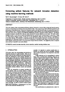
Figure 1.1 shows the relative distributions of the feature sets grouped to their audio descriptor’s origin when expanding the feature space from 50 top-ranked features to 500 top-ranked features. The number of features in total is 1450. Comparing ranks we notice that the top 50 ranks of the English database are occupied by intensity, spectrals and predominantly loudness features only. Pitch, formants and MFCC descriptors are not generating top rank features within the top 100 ranks. However, beyond this point pitch features become much more important for the English database than for the German. Table 1.2 already suggests that the different audio descriptor groups are of more equally weighted importance for the German database than they are for the English one. Also the feature distribution in the topranks suggest a more heterogeneous distribution in the German set. In general it seems as for the German set loudness and MFCCs are building the most important descriptors. The more features the more important becomes the MFCC contours. Note that also here the absolute number of MFCCs features affects the distribution more and more when the feature space expands.
17
Experiments and Results
As we expand the feature space for the English database three descriptor groups are of most importance: loudness, MFCC and pitch. Also cross-comparing the languages it seems that loudness is of higher impact for the English language as there are consistently more loudness features among all sizes of feature spaces for the English language. On the opposite, MFCC descriptors are more important to the German language. Note that these charts do not tell about how good the classification would be. This issue is discussed in the following Section. Figure 1.1. tures.
Feature group distribution group from top-50 until top-500 ranked fea-
distribution in percent
1
other pitch formant intensity loudness MFCC spectrals
0.8 0.6 0.4 0.2 0
50
100
150
200 250 300 350 number of features
400
450
500
400
450
500
(a) German corpus
distribution in percent
1 0.8 0.6 0.4 0.2 0
50
100
150
200 250 300 350 number of features (b) English corpus
8.2
Optimal Feature Sets
Table 1.2 already gives the f1-measurements for classification of features derived from separated audio descriptor groups. To obtain better
18Salient Features for Anger Recognition in German and English IVR Portals results we are now looking for the best combination of features from all descriptor groups. We thus need to find the parameters, i.e. the optimal number of features and the actual features included in that set. We make use of the IGR ranking again. Moving along the top ranks we incrementally admit a rising number of top-ranked features for classification. As expected, the scores predominantly rise as we start expanding the feature space. At a certain point no relevant information seem to be added when including more top-ranked features. In this phase, the scores seem to remain at a certain level showing some jitter. After including even more features we notice an overall decrease of performance again. Figure 1.2 shows the development of f1-measurement by incremental expansion. 78 English Database German Database
77
f1 in percent
76 75 74 73 72 71 70
33
66
99
132 165 198 231 264 297 330 363 number of top−ranked features in feature space
Figure 1.2.
396
429
462
495
Determination of optimal feature set size.
The optimal number of top-ranked features to include into the feature space resulted in 231 for the German database and 264 for the English database. Looking at figure 1.1 once more we can clearly see that on basis of the English database there is a higher number of pitch and loudness features in the top 250 feature space whereas in the German database more MFCC features can be found. Note that the saw-like shape of the graphs in Figure 1.2 indicate a non-optimal ranking since some feature inclusions seem to harm the performance. This is because the IGR filter uses heuristics to estimate the gain of information a single feature offers. Also any feature combination effects are not considered by the filter, although it is known that features that are less discriminative can develop high discrimination when
19
Discussion
integrated into a set. However, in the present experiments the IGR filter estimates the gain of single features independent from any set effects. Regarding the magnitude of the jitter we can see that it is as low as approx. 1% which after all proves a generally reasonable ranking. Regarding other requirements, as to lower to computational costs, one could also stop at the first local maximum of the f1 curves resulting in a reduced feature set of 66 features for the English and 165 features for the German database without losing more than 1% f1.
8.3
Optimal Classification
In a final step we adjusted the complexity of our classification algorithm which results in a best score of 78.2 f1 for the English and 74.7 f1 for the German database. All parameter settings were obtained by cross-validation evaluation. Previous studies on both corpora yielded a much lower performance compared to our new findings. The former system described in (Schmitt et al., 2009) with the English database reached 72.6% f1 while the system described in (Burkhardt et al., 2009) developed for the German database reached 70% f1. The performance gain on the training set of respectively 5.6% and 4.7% f1 in our study can be attributed to the employment of the enhanced feature sets and the feature selection by IGR filtering. Applied to the holdout sets we obtain figures presented in Table 1.4. For both languages the models capture more of Non-Anger information than of Anger information. Consequently the F-measure of the Anger class is always lower than the one of the Non-Anger class. We also see a better recall of Anger in English language. At the same time we see a better precision in German classification. After all, the overall performance of the final systems proved to be equivalently high. Note, that for given the class distribution of roughly 33/66 split in the test set constant classification into the majoritiy class would result in approx. 40% f1.
Table 1.4.
System performance figures on test sets.
Database
Class
Recall
Precision
F-measure
f1-measure
German
Non-Anger Anger
88.9% 63.7%
84.9% 72.0%
86.7% 67.6%
77.2%
English
Non-Anger Anger
82.3% 72.8%
86.0% 67.0%
84.1% 69.8%
77.0%
20Salient Features for Anger Recognition in German and English IVR Portals
9.
Discussion
Comparing classification scores we observe comparable results for both languages. Also the number of features needed for a reasonable anger classification seems similar. The difference in performance between test and train sets indicates that the calculated scores are reliable. Absolute scores prove a good overall classification success. Computational complexity can be reduced considerably without losing much classification score. However, we found differences in feature space setup in between the languages. The following Section presents possible explanations and discussion questions.
Signal Quality. One hypothesis for explaining the differences in feature distribution could be that callers may have dialed in via different transmission channels using different encoding paradigms. While the English database mostly comprises calls that were routed through land line connections the German database accounts for a greater share of mobile telephony transmission channels. Because fixed line connections transmit usually less compressed speech it can be assumed that there is more information retained in it. However, it is hard to conclude from the signal quality to the impact on our anger recognition task. More information transmitted does not automatically mean more relevance to anger classification. Speech Length. Another hypothesis for explaining the differences in the results could be the discrepancy in average turn length. The turn length can have a huge effect on statistics when applying a static feature length classification strategy. To estimate the impact of the average turn length we subsampled the German database to match the English average turn length. We processed the sub-samples analog to the original database. As a result we obtain major differences in the ranking list when operating on the shorter subset. While MFCC features account for roughly 35% in the original ranked German feature set the number drops to 22% on the subset. Accordingly, this figure becomes closer to the figure of 18% when working on the English corpus. Consequently we can hypothesize that the longer the turn the more important the MFCC features become. A possible explanation could be the increasing independence of the MFCC from the spoken context when drawing features on turn length. Though 70% of the MFCC features on the original set are also among the top ranked features on the subset the differences seem to be concentrated on the features from voiced speech parts. Also the higher MFCC coefficients seem to be affected from replacement. Further
21
Conclusion
experiments showing the impact of inter-lingual feature replacements in terms of classification scores can be found in (Polzehl et al., 2010). On the other hand, loudness and pitch features tend to remain on the original ranks when manipulating the average turn length. After all we still observe a large difference between the German and the English database when looking at pitch features. Sub-sampling did not have any significant effect here. Consequently this difference is not correlated with the average turn length. There is no clear effect from band limitation of the different transmition channels visible. Pitch estimation by autocorrelation re-constructs the pitch into similar intervals for both databases. On basis of these findings we can further hypothesize that there might exist a larger difference in emotional pitch usage in between German and English language at a linguistic level. In English language pitch variations might have a generally larger connection to vocal anger expression than in German.
Speech Transcription. Finally the procedures of training the labelers and the more precise differences in IVR design and dialogue domain could be considered as possible factors of influence as well. Also, as the English database offers a higher value of inter labeler agreement we would expect a better classification score for it. After all, though the classification results on the training sets mirror this difference they seem very balanced when classifying on the test sets. However, a difference in performance between test and train sets which accounts for less than 4% seems to indicate reasonable and reliable results for our anger recognition system on both corpora.
10.
Conclusion
We have shown that detecting angry utterances from IVR speech by acoustic measurements in English language is similar to detecting those utterances in German language. We have set up a large variety of acoustic and prosodic features. After applying IGR filter based ranking we compared the distribution of the features for both languages. Working with both languages we determine an absolute optimum when including 231 (German database) and 264 (English database) top-ranked features into the feature space. With respect of the maximum feature set size of 1450 these numbers are very close. When chosing the optimum number of features for each language, the relative importance of feature groups is also similar. Features derived from filtering in the spectral domain, e.g. MFCC, loudness, seem to be most promising for both databases. They account for more than 50% of all features. However, MFCCs occur more frequently under the
22Salient Features for Anger Recognition in German and English IVR Portals top-ranked features when operating on the German database, while operating on the English database loudness features are more frequently among top ranks. Another difference lies within the impact of pitch features. Although they are not among the top 50 features they become more and more important when including up to 300 features for the English language. They account for roughly 25% when trained on the English database while the number is as small as roughly 10% when trained on the German corpus. In terms of classification scores we obtain equally high f1 scores of approx. 77% for both languages. The classification baseline, which is given by constant majority class voting, is approx. 40% f1. Our results clearly outperform the baseline and previous versions of our anger recognition system. Moreover, the absolute height of achieved classification scores opens up deployment possibilities for real life applications.
Acknowledgments The authors wish to thank Prof. Sebastian M¨oller, Prof. Wolfgang Minker, Dr. Felix Burkhardt, Dr. Joachim Stegmann, Dr. David S¨ undermann, Dr. Roberto Pieraccini and Dr. Jackson Liscombe for their encouragement and support. The authors also wish to thank their colleagues at Quality and Usability Lab of Technische Universit¨at Berlin / Deutsche Telekom Laboratories, the Dialogue Systems Group of the Institute of Information Technology at University of Ulm and the Language Technologies Institute of Carnegie Mellon University, Pittsburgh for support and insightful discussions.
References
Batliner, A., Fischer, K., Huber, R., Spilker, J., and N¨oth, E. (2000). Desperately Seeking Emotions: Actors, Wizards, and Human Beings. In ISCA Workshop on Speech and Emotion. Boersma, P. and Weenink, D. (2009). Praat: Doing Phonetics by Computer. Burkhardt, F., Polzehl, T., Stegmann, J., Metze, F., and Huber, R. (2009). Detecting Real Life Anger. In ICASSP. Burkhardt, F., Rolfes, M., Sendlmeier, W., and Weiss, B. (2005a). A Database of German Emotional Speech. In Interspeech. ISCA. Burkhardt, F., van Ballegooy, M., and Huber, R. (2005b). An EmotionAware Voice Portal. In Proceedings of Electronic Speech Signal Processing ESSP. Davies, M. and Fleiss, J. (1982). Measuring Agreement for Multinomial Data. volume 38. Duda, R. O., Hart, P. E., and Stork, D. G. (2000). Pattern Classification. John Wiley & Sons, 2nd edition. Enberg, I. S. and Hansen, A. V. (1996). Documentation of the Danish Emotional Speech Database. Technical report, Aalborg University, Denmark. Fastl, H. and Zwicker, E. (2005). Psychoacoustics: Facts and Models. Springer, Berlin, 3rd edition. Lee, C. M. and Narayanan, S. S. (2005). Toward Detecting Emotions in Spoken Dialogs. IEEE Transactions on Speech and Audio Processing, 13:293–303. Lee, F.-M., Li, L.-H., and Huang, R.-Y. (2008). Recognizing Low/High Anger in Speech for Call Centers. In International Conference on Signal Processing, Robotics and Automation, pages 171–176. World Scientific and Engineering Academy and Society (WSEAS). Liscombe, J., Riccardi, G., and Hakkani-T¨ ur, D. (2005). Using Context to Improve Emotion Detection in Spoken Dialog Systems. In Interspeech, pages 1845–1848.
24Salient Features for Anger Recognition in German and English IVR Portals Metze, F., Englert, R., Bub, U., Burkhardt, F., and Stegmann, J. (2008). Getting Closer: Tailored HumanComputer Speech Dialog. Universal Access in the Information Society. Metze, F., Polzehl, T., and Wagner, M. (2009). Fusion of Acoustic and Linguistic Speech Features for Emotion Detection. In International Conference on Semantic Computing (ICSC). Nobuo, S. and Yasunari, O. (2007). Emotion recognition using melfrequency cepstral coefficients. Information and Media Technologies, 2:835–848. Polzehl, T., Schmitt, A., and Metze, F. (2010). Approaching MultiLingual Emotion Recognition from Speech - On Language Dependency of Acoustic/Prosodic Features for Anger Detection. In SpeechProsody, Chicago, U.S.A. Polzehl, T., Sundaram, S., Ketabdar, H., Wagner, M., and Metze, F. (2009). Emotion Classification in Children’s Speech Using Fusion of Acoustic and Linguistic Features. In Interspeech. Press, W.H.and Teukolsky, W., Vetterling, W., and Flannery, B. (1992). Numerical Recipes in C. Cambridge, University Press, 2nd edition. Rabiner, L. and Sambur, M. R. (1975). An Algorithm for Determining the Endpoints of Isolated Utterances. The Bell System Technical Journal, 56:297–315. Schmitt, A., Heinroth, T., and Liscombe, J. (2009). On NoMatchs, NoInputs and BargeIns: Do Non-Acoustic Features Support Anger Detection? In SIGDIAL Meeting on Discourse and Dialogue, London, UK. Association for Computational Linguistics. Schuller, B. (2006). Automatische Emotionserkennung aus Sprachlicher und manueller Interaktion. Dissertation, Technische Universit¨at M¨ unchen, M¨ unchen. Schuller, B., Batliner, A., Steidl, S., and Seppi, D. (2009). Emotion Recognition from Speech: Putting ASR in the Loop. In IEEE International Conference on Acoustics, Speech and Signal Processing (ICASSP). Shafran, I. and Mohri, M. (2005). A Comparison of Classifiers for Detecting Emotion from Speech. In IEEE International Conference on Acoustics, Speech and Signal Processing (ICASSP). Shafran, I., Riley, M., and Mohri, M. (2003). Voice Signatures. In Automatic Speech Recognition and Understanding, 2003. ASRU ’03. 2003 IEEE Workshop on, pages 31–36. Shannon, C. E. (1948). A Mathematical Theory of Communication. Bell System Technical Journal, 27. Steidl, S. (2009). Automatic Classification of Emotion-Related User States in Spontaneous Children’s Speech. PhD thesis.
REFERENCES
25
Steidl, S., Levit, M., Batliner, A., N¨oth, E., and Niemann, H. (2005). ”Of All Things the Measure is Man” - Classification of Emotions and Inter-Labeler Consistency. In IEEE, editor, International Conference on Acoustics, Speech, and Signal Processing (ICASSP), pages 317– 320. Vapnik, V. and Cortes, C. (1995). Support Vector Networks. Machine Learning, 20:273–297. Vlasenko, B. and Wendemuth, A. (2007). Tuning Hidden Markov Model for Speech Emotion Recognition. In 36. Deutsche Jahrestagung f¨ ur Akustik (DAGA). Wells, J. C. (1982). Accents of English, volume 1–3. Cambridge University Press. Witten, I. and Frank, F. (2005). Data Mining: Practical Machine Learning Tools and Techniques (Second Edition). Yacoub, S., Simske, S., Lin, X., and Burns, J. (2003). Recognition of Emotions in Interactive Voice Response Systems. In Eurospeech, Geneva, pages 1–4.