For each of the options, an email is sent to a random sample of 5,000 recipients to ... of whether the email was opened are analyzed and a logistical regression ...
Chapter 24 Logistic Regression Content list Purpose of logistic regression Assumptions of logistic regression The logistic regression equation Interpreting log odds and odds ratio Model fit and likelihood function SPSS activity – a logistic regression analysis
568 569 570 573 574 575
By the end of this chapter you will understand: 1 The purposes of logistic regression. 2 How to use SPSS to perform logistic regression. 3 How to interpret the SPSS printout of logistic regression.
Introduction This chapter extends our ability to conduct regression, in this case where the DV is a nominal variable. Our previous studies on regression have been limited to scale data DVs.
The purpose of logistic regression The crucial limitation of linear regression is that it cannot deal with DV’s that are dichotomous and categorical. Many interesting variables in the business world are dichotomous: for example, consumers make a decision to buy or not buy, a product may pass or fail quality control, there are good or poor credit risks, an employee may be promoted or not. A range of regression techniques have been developed for analysing data with categorical dependent variables, including logistic regression and discriminant analysis (DA) (Chapter 25). Logistical regression is regularly used rather than DA when there are only two categories of the dependent variable. Logistic regression is also easier to use with SPSS than DA when there is a mixture of numerical and categorical IV’s, because it includes procedures for generating the necessary dummy variables automatically, requires fewer assumptions, and is more statistically robust. DA strictly requires the continuous independent variables
LOGISTIC REGRESSION 569
(though dummy variables can be used as in multiple regression). Thus, in instances where the independent variables are categorical, or a mix of continuous and categorical, and the DV is categorical, logistic regression is necessary.
Logistic regression. Determines the impact of multiple independent variables presented simultaneously to predict membership of one or other of the two dependent variable categories.
Since the dependent variable is dichotomous we cannot predict a numerical value for it using logistic regression, so the usual regression least squares deviations criteria for best fit approach of minimizing error around the line of best fit is inappropriate. Instead, logistic regression employs binomial probability theory in which there are only two values to predict: that probability (p) is 1 rather than 0, i.e. the event/person belongs to one group rather than the other. Logistic regression forms a best fitting equation or function using the maximum likelihood method, which maximizes the probability of classifying the observed data into the appropriate category given the regression coefficients. We will avoid the more complicated mathematics of this. Like ordinary regression, logistic regression provides a coefficient ‘b’, which measures each IV’s partial contribution to variations in the DV. The goal is to correctly predict the category of outcome for individual cases using the most parsimonious model. To accomplish this goal, a model (i.e. an equation) is created that includes all predictor variables that are useful in predicting the response variable. Variables can, if necessary, be entered into the model in the order specified by the researcher in a stepwise fashion like regression. There are two main uses of logistic regression: •
•
The first is the prediction of group membership. Since logistic regression calculates the probability of success over the probability of failure, the results of the analysis are in the form of an odds ratio. Logistic regression also provides knowledge of the relationships and strengths among the variables (e.g. marrying the boss’s daughter puts you at a higher probability for job promotion than undertaking five hours unpaid overtime each week).
Assumptions of logistic regression • • • •
Logistic regression does not assume a linear relationship between the dependent and independent variables. The dependent variable must be a dichotomy (2 categories). The independent variables need not be interval, nor normally distributed, nor linearly related, nor of equal variance within each group. The categories (groups) must be mutually exclusive and exhaustive; a case can only be in one group and every case must be a member of one of the groups.
570
EXTENSION CHAPTERS ON ADVANCED TECHNIQUES
•
Larger samples are needed than for linear regression because maximum likelihood coefficients are large sample estimates. A minimum of 50 cases per predictor is recommended.
A non-mathematical illustration of logistic regression The dependent variable we are attempting to predict is whether an unsolicited email providing an emailed offer is opened or not by the recipient. There are two independent variables: • •
Presence or absence of recipient’s first name in the subject line. Presence or absence of the offer in the subject line.
Thus there are four possible combinations of interest: • • • •
Presence of first name, presence of offer in subject line. Absence of first name, presence of offer in subject line. Presence of first name, absence of offer in subject line. Absence of first name, absence of offer in subject line
For each of the options, an email is sent to a random sample of 5,000 recipients to ensure a low margin of error and high level of confidence. After a minimum of eight hours, results of whether the email was opened are analyzed and a logistical regression equation is generated for each of the options. Each equation predicts the impact of the independent variables on encouraging the consumer to take the desired action: opening and reading the email. You are able to determine which combination of the independent variables leads consumers to open the email most frequently. This analysis could also be run against individual customer segments. Some customer segments may respond to a combination of independent variables to which other customer segments are not responsive. For example, you might find that the independent variable of first name present only had a positive impact on recipients who were 39 and younger; the independent variable of first name present with no offer had no impact on recipients 40 and older. Then you know which variables to use or not when sending emails to recipients of different age groups.
The logistic regression equation While logistic regression gives each predictor (IV) a coefficient ‘b’ which measures its independent contribution to variations in the dependent variable, the dependent variable can only take on one of the two values: 0 or 1. What we want to predict from a knowledge of relevant independent variables and coefficients is therefore not a numerical value of a dependent variable as in linear regression, but rather the probability (p) that it is 1 rather than 0 (belonging to one group rather than the other). But even to use probability as the dependent variable is unsound, mainly because numerical predictors may be unlimited in range. If we expressed p as a linear function of investment,
LOGISTIC REGRESSION 571
we might then find ourselves predicting that p is greater than 1 (which cannot be true, as probabilities can only take values between 0 and 1). Additionally, because logistic regression has only two y values – in the category or not in the category – a straight line best fit (as in linear regression) is not possible to draw. Consider the following hypothetical example: 200 accountancy first year students are graded on a pass-fail dichotomy on the end of the semester accountancy exam. At the start of the course, they all took a maths pre-test with results reported in interval data ranging from 0–50 – the higher the pretest score the more competency in maths. Logistic regression is applied to determine the relationship between maths pretest score (IV or predictor) and whether a student passed the course (DV). Students who passed the accountancy course are coded 1 while those who failed are coded 0. We can see from Figure 24.1 of the plotted ‘x’s’ that there is somewhat greater likelihood that those who obtained above average to high score on the maths test passed the accountancy course, while below average to low scorers tended to fail. There is also an overlap in the middle area. But if we tried to draw a straight (best fitting) line, as with linear regression, it just would not work, as intersections of the maths results and pass/fail accountancy results form two lines of x’s, as in Figure 24.1. The solution is to convert or transform these results into probabilities. We might compute the average of the Y values at each point on the X axis. We could then plot the probabilities of Y at each value of X and it would look something like the wavy graph line superimposed on the original data in Figure 24.2. This is a smoother curve, and it is easy to see that the probability of passing the accountancy course (Y axis) increases as values of X increase. What we have just done is transform the scores so that the curve now fits a cumulative probability curve, i.e. adding each new probability to the existing total. As you can see, this curve is not a straight line; it is more of an s-shaped curve. Predicted values are interpreted as probabilities and are now not just two conditions with a value of either 0 or 1 but continuous data that can take any value from 0 to 1. The slope of the curve in Figure 24.2 is low at the lower and upper extremes of the independent variable and greatest in the middle where it is most sensitive. In the middle, of course, are a number of cases that are out of order, in the sense that there is an overlap with average maths scores in both accountancy pass and fail categories, while at the extremes are Pass 1
xx x x xx xxxxxxxxxxxxxx
Y
Fail
0
xxxxxxxxxxxx x xx x x xx x x Independent Variable Maths Score (X)
Figure 24.1 Maths results of 200 accountancy students plotted against the pass-fail categories.
572
EXTENSION CHAPTERS ON ADVANCED TECHNIQUES
1
xx x x xx xxxxxxxxxxxxxx
P
0
xxxxxxxxxxxx x xx x x xx x x Independent Variable Maths Score
Figure 24.2 Maths results plotted against probability of allocation to pass/fail categories.
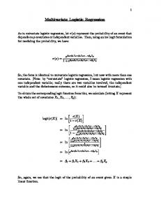
cases which are almost universally allocated to their correct group. The outcome is not a prediction of a Y value, as in linear regression, but a probability of belonging to one of two conditions of Y, which can take on any value between 0 and 1 rather than just 0 and 1 in Figure 24.1. Unfortunately a further mathematical transformation – a log transformation – is needed to normalize the distribution. You met this in Chapter 8, where log transformations and sq. root transformations moved skewed distributions closer to normality. So what we are about to do is not uncommon. This log transformation of the p values to a log distribution enables us to create a link with the normal regression equation. The log distribution (or logistic transformation of p) is also called the logit of p or logit(p). Logit(p) is the log (to base e) of the odds ratio or likelihood ratio that the dependent variable is 1. In symbols it is defined as: logit (p) = log[p / (1 − p)] = ln [p / (1 − p)] Whereas p can only range from 0 to 1, logit(p) scale ranges from negative infinity to positive infinity and is symmetrical around the logit of .5 (which is zero). Formula 24.1 below shows the relationship between the usual regression equation (a + bx … etc.), which is a straight line formula, and the logistic regression equation. The form of the logistic regression equation is: ⎡ p(x) ⎤ logit [p(x)] = log ⎢ ⎥ = a + b1x1 + b2 x 2 + b3 x3 … ⎢ 1 − p(x) ⎥ This looks just like a linear regression and although logistic regression finds a ‘best fitting’ equation, just as linear regression does, the principles on which it does so are rather different. Instead of using a least-squared deviations criterion for the best fit, it uses a maximum likelihood method, which maximizes the probability of getting the observed results given the fitted regression coefficients. A consequence of this is that the goodness of fit and overall significance statistics used in logistic regression are different
LOGISTIC REGRESSION 573
from those used in linear regression. p can be calculated with the following formula (formula 24.2) which is simply another rearrangement of formula 24.1: p=
exp
(a + b1 x1 + b2 x 2 + b3 x3 …)
1 + exp
(a + b1 x1 + b2 x 2 + b3 x3 …)
formula 24.2
Where: p = the probability that a case is in a particular category, exp = the base of natural logarithms (approx 2.72), a = the constant of the equation and, b = the coefficient of the predictor variables. Formula 24.2 involves another mathematic function, exp, the exponential function. ln, the natural logarithm, and exp are opposites. The exponential function is a constant with the value of 2.71828182845904 (roughly 2.72). When we take the exponential function of a number, we take 2.72 raised to the power of the number. So, exp(3) equals 2.72 cubed or (2.72)3 = 20.09. The natural logarithm is the opposite of the exp function. If we take ln(20.09), we get the number 3. These are common mathematical functions on many calculators. Don’t worry, you will not have to calculate any of this mathematical material by hand. I have simply been trying to show you how we get from a regression formula for a line to the logistic analysis.
Logistic regression – involves fitting an equation of the form to the data: logit(p) = a + b1x1 + b2x2 + b3x3 + …
Interpreting log odds and the odds ratio What has been presented above as mathematical background will be quite difficult for some of you to understand, so we will now revert to a far simpler approach to consider how SPSS deals with these mathematical complications. The Logits (log odds) are the b coefficients (the slope values) of the regression equation. The slope can be interpreted as the change in the average value of Y, from one unit of change in X. In SPSS the b coefficients are located in column ‘B’ in the ‘Variables in the Equation’ table. Logistic regression calculates changes in the log odds of the dependent, not changes in the dependent value as OLS regression does. For a dichotomous variable the odds of membership of the target group are equal to the probability of membership in the target group divided by the probability of membership in the other group. Odds value can range from 0 to infinity and tell you how much more likely it is that an observation is a member of the target group rather than a member of the other group. If the probability is 0.80, the odds are 4 to 1 or .80/.20; if the probability is 0.25, the odds are .33 (.25/.75). If the probability of membership in the target group is .50, the odds are 1 to 1 (.50/.50), as in coin tossing when both outcomes are equally likely.
574
EXTENSION CHAPTERS ON ADVANCED TECHNIQUES
Another important concept is the odds ratio (OR), which estimates the change in the odds of membership in the target group for a one unit increase in the predictor. It is calculated by using the regression coefficient of the predictor as the exponent or exp. Assume in the example earlier where we were predicting accountancy success by a maths competency predictor that b = 2.69. Thus the odds ratio is exp2.69 or 14.73. Therefore the odds of passing are 14.73 times greater for a student, for example, who had a pre-test score of 5, than for a student whose pre-test score was 4. SPSS actually calculates this value of the ln(odds ratio) for us and presents it as EXP(B) in the results printout in the ‘Variables in the Equation’ table. This eases our calculations of changes in the DV due to changes in the IV. So the standard way of interpreting a ‘b’ in logistic regression is using the conversion of it to an odds ratio using the corresponding exp(b) value. As an example, if the logit b = 1.5 in the B column of the ‘Variables in the Equation’ table, then the corresponding odds ratio (column exp(B)) quoted in the SPSS table will be 4.48. We can then say that when the independent variable increases one unit, the odds that the case can be predicted increase by a factor of around 4.5 times, when other variables are controlled. As another example, if income is a continuous explanatory variable measured in ten thousands of dollars, with a ‘b’ value of 1.5 in a model predicting home ownership = 1, no home ownership = 0. Then since exp(1.5) = 4.48, a 1 unit increase in income (one $10,000 unit) increases the odds of home ownership about 4.5 times. This process will become clearer through following through the SPSS logistic regression activity below.
Model fit and the likelihood function Just as in linear regression, we are trying to find a best fitting line of sorts but, because the values of Y can only range between 0 and 1, we cannot use the least squares approach. The Maximum Likelihood (or ML) is used instead to find the function that will maximize our ability to predict the probability of Y based on what we know about X. In other words, ML finds the best values for formula 24.1 above. Likelihood just means probability. It always means probability under a specified hypothesis. In logistic regression, two hypotheses are of interest: • •
the null hypothesis, which is when all the coefficients in the regression equation take the value zero, and the alternate hypothesis that the model with predictors currently under consideration is accurate and differs significantly from the null of zero, i.e. gives significantly better than the chance or random prediction level of the null hypothesis.
We then work out the likelihood of observing the data we actually did observe under each of these hypotheses. The result is usually a very small number, and to make it easier to handle, the natural logarithm is used, producing a log likelihood (LL). Probabilities are always less than one, so LL’s are always negative. Log likelihood is the basis for tests of a logistic model. The likelihood ratio test is based on –2LL ratio. It is a test of the significance of the difference between the likelihood ratio (–2LL) for the researcher’s model with predictors (called model chi square) minus the likelihood ratio for baseline model with
LOGISTIC REGRESSION 575
only a constant in it. Significance at the .05 level or lower means the researcher’s model with the predictors is significantly different from the one with the constant only (all ‘b’ coefficients being zero). It measures the improvement in fit that the explanatory variables make compared to the null model. Chi square is used to assess significance of this ratio.
The likelihood ratio test. This tests the difference between –2LL for the full model with predictors and –2LL for initial chi-square in the null model.
When probability fails to reach the 5% significance level, we retain the null hypothesis that knowing the independent variables (predictors) has no increased effects (i.e. make no difference) in predicting the dependent. We will now have a look at the concepts and indices introduced above by running an SPSS logistic regression and see how it all works in practice.
SPSS activity – a logistic regression analysis Access SPSS Ch 24 Data File A. This file contains data from a survey of home owners conducted by an electricity company about an offer of roof solar panels with a 50% subsidy from the state government as part of the state’s environmental policy. The variables involve household income measured in units of a thousand dollars, age, monthly mortgage, size of family household, and whether the householder would take or decline the offer. Please follow the instructions below and conduct a logistic regression to determine whether family size and monthly mortgage will predict taking or declining the offer. Click Analyze >> Regression >> Binary Logistic. Select the grouping variable (the variable to be predicted) which must be a dichotomous measure and place it into the Dependent box (Fig. 24.3). For this example it is ‘take solar panel offer’. The convention for binomial logistic regression is to code the dependent class of greatest interest as 1 and the other class as 0, because the coding will affect the odds ratios and slope estimates. 3 Enter your predictors (IV’s) into the Covariates box. These are ‘family size’ and ‘mortgage’. Do not alter the default method of Enter unless you wish to run a Stepwise logistic regression. Forward selection is the usual option for a stepwise regression, starting with the constant-only model and adding variables one at a time. The forward stepwise logistic regression method utilizes the likelihood ratio test (chi square difference) which tests the change in –2LL between steps to determine automatically which variables to add or drop from the model. This is considered useful only for exploratory purposes. Selecting model variables on a theoretic basis and using the Enter method is preferred. 4 Should you have any categorical predictor variables, click on ‘Categorical’ button and enter it (there is none in this example). The define categorical variables box is displayed as in Figure 24.4. SPSS asks what coding methods you would like for the
1 2
576
EXTENSION CHAPTERS ON ADVANCED TECHNIQUES
Figure 24.3 Logistic regression dialogue box.
Figure 24.4 Categorical variables box.
LOGISTIC REGRESSION 577
predictor variable (under the Categorical button), and there are several options to choose from. For most situations, choose the ‘indicator’ coding scheme (it is the default). You can choose to have the first or last category of the variable as your baseline reference category. Usually, the absence of the factor is coded as 0, and the presence of the factor is coded 1. If so, you want to make sure that the first category (the one of the lowest value) is designated as the reference category in the categorical dialogue box. SPSS will convert categorical variables to dummy variables automatically. The class of greatest interest should be the last class (1 in a dichotomous variable for example). 5 Click on Options button and select Classification Plots, Hosmer-Lemeshow Goodness Of Fit, Casewise Listing Of Residuals and select Outliers Outside 2sd. Retain default entries for probability of stepwise, classification cutoff and maximum iterations (Fig. 24.5). 6 Continue then OK.
Figure 24.5 Options dialogue box.
Interpretation of printout Table 24.1 The first few tables in your printout are not of major importance. The first one to take note of is the Classification table (Table 24.1) in Block 0 Beginning Block. 1
Block 0: Beginning Block. Block 0 presents the results with only the constant included before any coefficients (i.e. those relating to family size and mortgage) are entered into the equation. Logistic regression compares this model with a model including all the predictors (family size and mortgage) to determine whether the latter model is more appropriate. The table suggests that if we knew nothing about our variables and guessed
578
EXTENSION CHAPTERS ON ADVANCED TECHNIQUES Table 24.1 The classification table Classification Tablea,b Predicted Take solar panel offer Observed Step 0
a b
take solar panel offer Overall Percentage
Decline offer
Take offer
0 0
14 16
decline offer take offer
Percentage correct .0 100.0 53.3
Constant is included in the model. The cut value is .500.
Table 24.2 Variables in the equation table Variables in the Equation
Step 0
Constant
B
S.E.
Wald
df
Sig.
Exp(B)
.134
.366
.133
1
.715
1.143
Score
df
Sig.
14.632 6.520 15.085
1 1 2
.000 .011 .001
Table 24.3 Variables not in the equation table Variables not in the Equation
Step 0
Variables Overall Statistics
Famsize Mortgage
that a person would not take the offer we would be correct 53.3% of the time. The variables not in the equation table tells us whether each IV improves the model (Table 24.3). The answer is yes for both variables, with family size slightly better than mortgage size, as both are significant and if included would add to the predictive power of the model. If they had not been significant and able to contribute to the prediction, then termination of the analysis would obviously occur at this point. 2 Block 1 Method = Enter. This presents the results when the predictors ‘family size’ and ‘mortgage’ are included. Later SPSS prints a classification table which shows how the classification error rate has changed from the original 53.3%. By adding the variables we can now predict with 90% accuracy (see Classification Table 24.8 below). The model appears good, but we need to evaluate model fit and significance as well. SPSS will offer you a variety of statistical tests for model fit and whether each of the independent variables included make a significant contribution to the model.
LOGISTIC REGRESSION 579 Table 24.4 Omnibus tests of model coefficients Omnibus Tests of Model Coefficients
Step 1
3
Step Block Model
Chi-square
df
Sig.
24.096 24.096 24.096
2 2 2
.000 .000 .000
Model chi-square. The overall significance is tested using what SPSS calls the Model Chi square, which is derived from the likelihood of observing the actual data under the assumption that the model that has been fitted is accurate. There are two hypotheses to test in relation to the overall fit of the model: H0 The model is a good fitting model. H1 The model is not a good fitting model (i.e. the predictors have a significant effect).
The difference between –2LL for the best-fitting model and –2LL for the null hypothesis model (in which all the b values are set to zero in block 0) is distributed like chi squared, with degrees of freedom equal to the number of predictors; this difference is the Model chi square that SPSS refers to. Very conveniently, the difference between – 2LL values for models with successive terms added also has a chi squared distribution, so when we use a stepwise procedure, we can use chi-squared tests to find out if adding one or more extra predictors significantly improves the fit of our model. The –2LL value from the Model Summary table below is 17.359. In our case model chi square has 2 degrees of freedom, a value of 24.096 and a probability of p < 0.000 (Table 24.4). Thus, the indication is that the model has a poor fit, with the model containing only the constant indicating that the predictors do have a significant effect and create essentially a different model. So we need to look closely at the predictors and from later tables determine if one or both are significant predictors. This table has 1 step. This is because we are entering both variables and at the same time providing only one model to compare with the constant model. In stepwise logistic regression there are a number of steps listed in the table as each variable is added or removed, creating different models. The step is a measure of the improvement in the predictive power of the model since the previous step. 4 Model Summary. Although there is no close analogous statistic in logistic regression to the coefficient of determination R2 the Model Summary Table 24.5 provides some approximations. Cox and Snell’s R-Square attempts to imitate multiple R-Square based Table 24.5 Model Summary Model Summary Step 1 a
−2 Log likelihood a
17.359
Cox & Snell R square
Nagelkerke R square
.552
.737
Estimation terminated at iteration number 8 because parameter estimates changed by less than .001.
580
EXTENSION CHAPTERS ON ADVANCED TECHNIQUES
on ‘likelihood’, but its maximum can be (and usually is) less than 1.0, making it difficult to interpret. Here it is indicating that 55.2% of the variation in the DV is explained by the logistic model. The Nagelkerke modification that does range from 0 to 1 is a more reliable measure of the relationship. Nagelkerke’s R2 will normally be higher than the Cox and Snell measure. Nagelkerke’s R2 is part of SPSS output in the ‘Model Summary’ table and is the most-reported of the R-squared estimates. In our case it is 0.737, indicating a moderately strong relationship of 73.7% between the predictors and the prediction. 5 H-L Statistic. An alternative to model chi square is the Hosmer and Lemeshow test which divides subjects into 10 ordered groups of subjects and then compares the number actually in the each group (observed) to the number predicted by the logistic regression model (predicted) (Table 24.7). The 10 ordered groups are created based on their estimated probability; those with estimated probability below .1 form one group, and so on, up to those with probability .9 to 1.0. Each of these categories is further divided into two groups based on the actual observed outcome variable (success, failure). The expected frequencies for each of the cells are obtained from the model. A probability (p) value is computed from the chi-square distribution with 8 degrees of freedom to test the fit of the logistic model. If the H-L goodness-of-fit test statistic is greater than .05, as we want for well-fitting models, we fail to reject the null hypothesis that there is no difference between observed and model-predicted values, implying that the model’s estimates fit the data at an acceptable level. That is, well-fitting models show non-significance on the H-L goodness-of-fit test. This desirable outcome of non-significance indicates that the model prediction does not significantly differ from the observed. The H-L statistic assumes sampling adequacy, with a rule of thumb being enough cases so that 95% of cells (typically, 10 decile groups times 2 outcome categories = 20 cells) have an expected frequency > 5. Our H-L statistic has a significance of .605 which means that it is not statistically significant and therefore our model is quite a good fit (Table 24.6) 6 Classification Table. Rather than using a goodness-of-fit statistic, we often want to look at the proportion of cases we have managed to classify correctly. For this we need to look at the classification table printed out by SPSS, which tells us how many of the cases where the observed values of the dependent variable were 1 or 0 respectively have been correctly predicted. In the Classification table (Table 24.8), the columns are the two predicted values of the dependent, while the rows are the two observed (actual) values of the dependent. In a perfect model, all cases will be on the diagonal and the overall percent correct will be 100%. In this study, 87.5% were correctly classified for the take offer group and 92.9% for the decline offer group. Overall 90% were correctly classified. This is a considerable improvement on the 53.3% correct classification with the constant model so we know that the model with predictors is a significantly better mode.
Table 24.6 Hosmer and Lemeshow test Hosmer and Lemeshow Test Step
Chi-square
df
Sig.
1
6.378
8
.605
LOGISTIC REGRESSION 581 Table 24.7 Contingency table for Hosmer and Lemeshow test Contingency Table for Hosmer and Lemeshow Test
Step 1
Take solar panel offer = decline offer
Take solar panel offer = take offer
Observed
Expected
Observed
Expected
Total
1 2 3 4 5 6 7
3 3 3 2 2 0 0
2.996 2.957 2.629 2.136 1.881 .833 .376
0 0 0 1 1 3 3
.004 .043 .371 .864 1.119 2.167 2.624
3 3 3 3 3 3 3
8
1
.171
2
2.829
3
9 10
0 0
.019 .000
3 3
2.981 3.000
3 3
But are both predictor variables responsible or just one of them? This is answered by the Variables in the Equation table. Table 24.8 Classification table Classification Tablea Predicted Take solar panel offer Observed Step 1
a
take solar panel offer Overall Percentage
decline offer take offer
Decline offer
Take offer
Percentage correct
13 2
1 14
92.9 87.5 90.0
The cut value is .500.
7
Variables in the Equation. The Variables in the Equation table (Table 24.9) has several important elements. The Wald statistic and associated probabilities provide an index of the significance of each predictor in the equation. The Wald statistic has a chi-square distribution. The simplest way to assess Wald is to take the significance values and if less than .05 reject the null hypothesis as the variable does make a significant contribution. In this case, we note that family size contributed significantly to the prediction (p = .013) but mortgage did not (p = .075). The researcher may well want to drop independents from the model when their effect is not significant by the Wald statistic (in this case mortgage).
582
EXTENSION CHAPTERS ON ADVANCED TECHNIQUES Table 24.9 Variables in the equation Variables in the Equation
Step 1a Famsize Mortgage Constant a
B
S.E.
Wald
df
Sig.
Exp(B)
2.399 .005 −18.627
.962 .003 8.654
6.215 3.176 4.633
1 1 1
.013 .075 .031
11.007 1.005 .000
Variable(s) entered on step 1: Famsize, Mortgage.
The Exp(B) column in Table 24.9 presents the extent to which raising the corresponding measure by one unit influences the odds ratio. We can interpret EXP(B) in terms of the change in odds. If the value exceeds 1 then the odds of an outcome occurring increase; if the figure is less than 1, any increase in the predictor leads to a drop in the odds of the outcome occurring. For example, the EXP(B) value associated with family size is 11.007. Hence when family size is raised by one unit (one person) the odds ratio is 11 times as large and therefore householders are 11 more times likely to belong to the take offer group. The ‘B’ values are the logistic coefficients that can be used to create a predictive equation (similar to the b values in linear regression) formula 24.2, page 573. In this example: Probability of a case =
e{( 2.399 × family size ) + (.0005 × mortgage ) − 18.627} 1 + e{( 2.399 × family size ) + (.005 × mortgage ) − 18.627}
Here is an example of the use of the predictive equation for a new case. Imagine a householder whose household size including themselves was seven and paying a monthly mortgage of $2,500. Would they take up the offer, i.e. belong to category 1? Substituting in we get: Probability of a case taking offer = =
e{(2.399 × 7) + (.005 × 2500) – 18.627} 1 + e{(2.399 × 7) + (.005 × 2500) – 18.627} e10.66
1 + e10.66 = 0.99
Therefore, the probability that a householder with seven in the household and a mortgage of $2,500 p.m. will take up the offer is 99%, or 99% of such individuals will be expected to take up the offer. Note that, given the non-significance of the mortgage variable, you could be justified in leaving it out of the equation. As you can imagine, multiplying a mortgage value by B adds a negligible amount to the prediction as its B value is so small (.005).
LOGISTIC REGRESSION 583
Effect size. The odds ratio is a measure of effect size. The ratio of odds ratios of the independents is the ratio of relative importance of the independent variables in terms of effect on the dependent variable’s odds. In our example family size is 11 times as important as monthly mortgage in determining the decision. 8
Classification Plot. The classification plot or histogram of predicted probabilities provides a visual demonstration of the correct and incorrect predictions (Table 24.10). Also called the ‘classplot’ or the ‘plot of observed groups and predicted probabilities’, it is another very useful piece of information from the SPSS output when one chooses ‘Classification plots’ under the Options button in the Logistic Regression dialogue box. The X axis is the predicted probability from .0 to 1.0 of the dependent being classified ‘1’. The Y axis is frequency: the number of cases classified. Inside the plot are columns of observed 1’s and 0’s (or equivalent symbols). The resulting plot is very useful for spotting possible outliers. It will also tell you whether it might be better to separate the two predicted categories by some rule other than the simple one SPSS uses, which is to predict value 1 if logit(p) is greater than 0 (i.e. if p is greater than .5). A better separation of categories might result from using a different criterion. We might also want to use a different criterion if the a priori probabilities of the two categories were very different (one might be winning the national lottery, for example), or if the costs of mistakenly predicting someone into the two categories differ (suppose the categories were ‘found guilty of fraudulent share dealing’ and ‘not guilty’, for example).
Look for two things: (1) A U-shaped rather than normal distribution is desirable. A U-shaped distribution indicates the predictions are well-differentiated with cases clustered at each end showing correct classification. A normal distribution indicates too many predictions close to the cut point, with a consequence of increased misclassification around the cut point which is not a good model fit. For these around .50 you could just as well toss a coin. (2) There should be few errors. The ‘t’s’ to the left are false positives. The ‘d’s’ to the right are false negatives. Examining this plot will also tell such things as how well the model classifies difficult cases (ones near p = .5). 9
Casewise List. Finally, the casewise list produces a list of cases that didn’t fit the model well. These are outliers. If there are a number of cases this may reveal the need for further explanatory variables to be added to the model. Only one case (No. 21) falls into this category in our example (Table 24.11) and therefore the model is reasonably sound. This is the only person who did not fit the general pattern. We do not expect to obtain a perfect match between observation and prediction across a large number of cases. No excessive outliers should be retained as they can affect results significantly. The researcher should inspect standardized residuals for outliers (ZResid in Table 24.11) and consider removing them if they exceed > 2.58 (outliers at the .01 level). Standardized residuals are requested under the ‘Save’ button in the binomial logistic regression dialog box in SPSS. For multinomial logistic regression, checking ‘Cell Probabilities’ under the ‘Statistics’ button will generate actual, observed, and residual values.
584
EXTENSION CHAPTERS ON ADVANCED TECHNIQUES
Table 24.10 Classification plot Step number: 1 Observed Groups and Predicted Probabilities 8
F R E Q U E N C Y
6
4
2
Predicte Prob : Group:
d d d d d d dd dd dd dd
d d
t t dt dt dd dd
d d
0
t t tt tt
d d
.25
.5
t t
.75
t t ttd t ttd t
t t t t t t t t t t t t 1
ddddddddddddddddddddddddddddddtttttttttttttttttttttttttttttt Predicted Probability is of Membership for take offer The Cut Value is .50 Symbols: d - decline offer t - take offer Each Symbol Represents .5 Cases
Table 24.11 Casewise list Casewise Listb Temporary variable
Observed
a b
Case
Selected statusa
21
S
Take solar panel offer
Predicted
Predicted group
Resid
ZResid
d**
.924
t
−.924
−3.483
S = Selected, U = Unselected cases, and = Misclassified cases. Cases with studentized residuals greater than 2.000 are listed. **
LOGISTIC REGRESSION 585
How to report your results You could model a write up like this: ‘A logistic regression analysis was conducted to predict take-up of a solar panel subsidy offer for 30 householders using family size and monthly mortgage payment as predictors. A test of the full model against a constant only model was statistically significant, indicating that the predictors as a set reliably distinguished between acceptors and decliners of the offer (chi square = 24.096, p < .000 with df = 2). Nagelkerke’s R2 of .737 indicated a moderately strong relationship between prediction and grouping. Prediction success overall was 90% (92.9% for decline and 87.5% for accept. The Wald criterion demonstrated that only family size made a significant contribution to prediction (p = .013). Monthly mortgage was not a significant predictor. EXP(B) value indicates that when family size is raised by one unit (one person) the odds ratio is 11 times as large and therefore householders are 11 more times likely to take the offer’. To relieve your stress Some parts of this chapter may have seemed a bit daunting. But remember, SPSS does all the calculations. Just try and grasp the main principles of what logistic regression is all about. Essentially, it enables you to: •
• •
see how well you can classify people/events into groups from a knowledge of independent variables; this is addressed by the classification table and the goodness-of-fit statistics discussed above; see whether the independent variables as a whole significantly affect the dependent variable; this is addressed by the Model Chi-square statistic. determine which particular independent variables have significant effects on the dependent variable; this can be done using the significance levels of the Wald statistics, or by comparing the –2LL values for models with and without the variables concerned in a stepwise format.
SPSS Activity. Now access SPSS Chapter 24 Data File A on the website, and conduct your own logistic regression analysis using age and family size as predictors for taking or declining the offer. Write out an explanation of the results and discuss in class.
What you have learned from this chapter Binomial (or binary) logistic regression is a form of regression which is used when the dependent is a dichotomy and the independents are of any type. The goal is to find the best set of coefficients so that cases that belong to a particular category will, when using the equation, (Continued)
586
EXTENSION CHAPTERS ON ADVANCED TECHNIQUES
have a very high calculated probability that they will be allocated to that category. This enables new cases to be classified with a reasonably high degree of accuracy as well. Logistic regression uses binomial probability theory, does not assume linearity of relationship between the independent variables and the dependent, does not require normally distributed variables, and in general has no stringent requirements. Logistic regression has many analogies to linear regression: logit coefficients correspond to b coefficients in the logistic regression equation, the standardized logit coefficients correspond to beta weights, and the Wald statistic, a pseudo R2 statistic, is available to summarize the strength of the relationship. The success of the logistic regression can be assessed by looking at the classification table, showing correct and incorrect classifications of the dependent. Also, goodness-of-fit tests such as model chi- square are available as indicators of model appropriateness, as is the Wald statistic to test the significance of individual independent variables. The EXP(B) value indicates the increase in odds from a one unit increase in the selected variable.
Review questions Qu. 24.1 Why are p values transformed to a log value in logistic regression? (a) (b) (c) (d) (e)
because p values are extremely small because p values cannot be analyzed because p values only range between 0 and 1 because p values are not normally distributed none of the above
Qu. 24.2 The Wald statistic is: (a) (b) (c) (d)
a beta weight equivalent to R2 a measure of goodness of fit a measure of the increase in odds
Qu. 24.3 Logistic regression is based on: (a) (b) (c) (d)
normal distribution Poisson distribution the sine curve binomial distribution
LOGISTIC REGRESSION 587
Qu. 24.4 Logistic regression is essential where, (a) (b) (c) (d)
both the dependent variable and independent variable(s) are interval the independent variable is interval and both the dependent variables are categorical the sole dependent variable is categorical and the independent variable is not interval there is only one dependent variable irrespective of the number or type of the independent variable(s)
Qu. 24.5 exp(B) in the SPSS printout tells us (a) (b) (c) (d)
the probability of obtaining the dependent variable value the significance of beta for each unit change in X what the change factor is for Y the significance of the Wald statistic
Qu. 24.6 Explain briefly why a line of best fit approach cannot be applied in logistic regression. Check your response in the material above. Qu. 24.7 Under what circumstances would you choose to use logistic regression? Check your response with the material above. Qu. 24.8 What is the probability that a householder with only two in the household and a monthly mortgage of $1,700 will take up the offer? Check your answer on the web site for this chapter.
Now access the Web page for Chapter 24 and check your answers to the above questions. You should also attempt the SPSS activity.
Additional reading Agresti, A. 1996. An Introduction to Categorical Data Analysis. John Wiley and Sons. Fox, J. 2000. Multiple and Generalized Nonparametric Regression. Thousand Oaks, CA: Sage Publications. Quantitative applications in the social sciences Series
588
EXTENSION CHAPTERS ON ADVANCED TECHNIQUES
No. 131. Covers non-parametric regression models for GLM techniques like logistic regression. Menard, S. 2002. Applied Logistic Regression Analysis (2nd edn). Thousand Oaks, CA: Sage Publications. Series: Quantitative Applications in the Social Sciences, No. 106 (1st edn), 1995. O’Connell, A. A. 2005. Logistic Regression Models for Ordinal Response Variables. Thousand Oaks, CA: Sage Publications. Quantitative applications in the social sciences, Volume 146. Pampel, F. C. 2000. Logistic Regression: A Primer. Sage quantitative applications in the Social Sciences Series #132. Thousand Oaks, CA: Sage Publications. Useful website Alan Agresti’s website, with all the data from the worked examples in his book: http://lib. stat.cmu.edu/datasets/agrest.