Chapter Two

Coaley-3941-Ch-02:Coaley-Sample.qxp

30/07/2009

8:05 PM

Page 23

PART 1 The Essential Tools of Psychological Measurement


30/07/2009

8:05 PM

Page 24


30/07/2009

8:05 PM

Page 25

2 The Basic Components – Scales and Items

Learning Objectives By the end of this chapter you should be able to: • Give an account of the different types of scale and items available for psychological assessment and discuss their advantages and limitations. • Explain and critically evaluate the principal approaches to item analysis using • Classical Item Analysis, Item Response Theory and Rasch modelling. • Understand scientific thinking about the nature of attitudes and their key characteristics. • Identify the different approaches to scaling and measurement of attitudes.

What is this Chapter About? This chapter deals with the basic underlying components of assessment – scales and items. Getting them right is crucial. Scales enable us to transform the responses of people into scores which provide a quantitative means of measuring characteristics – and measurement lies at the heart of accurate assessment. There are different types of scale available, not just in their level of precision but also in terms of their use. The second component – the items – could effectively form the units of measurement on the scale and provides the motor for measurement by generating responses. Their quantity and quality are also basic requirements for good testing. Items and scales need to work in an effective manner if we are to have acceptable methods. We will consider contrasting approaches to item analysis. Lastly, we will explore how different scales and methods have been applied to attitude measurement. At the end you should be able to draw a line between measures based on


30/07/2009

8:05 PM

Page 26

• • • An Introduction to Psychological Assessment and Psychometrics • • • good scales and sufficient items from those which are flawed. Measurement is the foundation stone of assessment.

What Kinds of Scales are Available? People differ in so many ways, whether in physical or psychological characteristics. These attributes, varying from person to person, are called variables (unlike constants which are fixed, such as the number of legs or ears we usually have), although a person can have only one value of a variable at any time. Variables are made up of intervals and are continuous, making it possible to measure them on scales. Some individual differences can be measured more precisely than others, depending upon the kind of scale used. But measuring psychological concepts raises a fundamental problem. There isn’t any external scale against which our scales can be judged. For example, in measuring height there are things like measuring tapes or sticks marked in standard units. Ultimately, these can be calibrated against an external standard measure kept in a laboratory at fixed temperature. The same thing can happen for some other kinds of measurement like weight/mass. But no similar external standard exists for psychological characteristics. There is not one perfect ability or personality measure sitting in splendid isolation in a laboratory somewhere. Yet there is a need for commonly agreed standards. Psychology has coped with this in a number of ways and there has been much thought about measurement (Michell, 1990; Kline, 1998). By far the most common method is through the use of a reference population or norm group. An individual is regarded as a member of the group and the score obtained can be compared to a mean score for all of the other members. In the case of some measures, such as cognitive or reasoning tests, all of the correct items are counted to give just one raw scale score (sometimes referred to simply as the raw score for a person). In this case the maximum possible response sets the limit of the raw score scale. For an ability test having 40 items, a person might have a raw score anywhere from 0 to 40. For other instruments, the items may be separated into two or more groups, each with its own raw score scale: • Specific ability or aptitude tests tend to keep their items separate, with a score for each test. Raw scores can then be summed to give an overall measure of general ability. • General ability or reasoning measures will mix different types of item together and create a single score for the overall test. • Personality and interest inventories will often mix all of the items together. Scoring keys or computer software separate the items belonging to different scales and give one score for each. It is important to note that the raw score, however it is calculated, is an absolute score because it doesn’t depend on or relate to the scores of others. In most instances this is • 26 •


30/07/2009

8:05 PM

Page 27

• • • The Basic Components – Scales and Items • • •

transformed into another score, for example a standard based upon 10 (sten scores) or a percentile (the level below which others in the norm group have scored) or even a grade (usually A to E, a purely arbitrary scale) which does relate the individual’s performance to responses in the reference population so as to provide a meaningful interpretation. In this way a score could be linked, say, to a population of people who have been diagnosed as suffering from depression, enabling us to determine a person’s comparable level. Scores related to how others perform are called relative scores. When it comes to the scales used, there are four kinds available: nominal, ordinal, interval and ratio scales:

Nominal Scales This is the most basic scale available. It is used for naming or describing things, for example by describing occupation, ethnic group, country of origin or sex (male = 1, female =2) in terms of numbers, although it can’t be used to indicate the order or magnitude of them. Nominal scales simply classify people into categories by labelling and are a convenient method of describing them as individuals or groups. Here are some examples of scales used to determine whether people belong in the same or different categories based on a particular attribute: 1 2

The number of people having each of the following eye colours: blue, hazel, brown, green, black. The number of people who have: bought this book, loaned it from a library, borrowed it from a friend, found it somewhere, or stolen it.

The problem with nominal scales is that only a limited number of transformations and statistics can be conducted on data. The categories are not ordered in any way and, therefore, they are different but cannot be compared quantitatively. Any amount of difference between them may not be known and the only calculations possible are based upon the number of people in each category (their frequencies) and proportions. The Chi-square test may also be used to understand any association between categories.

Ordinal Scales These provide a more precise level of measurement than nominal scales and place people in some kind of hierarchical order by assigning numbers or rank ordering. They indicate an individual’s position regarding some variable where this can be ordered, for example from low to high or from first to last as in a competition. This can help decide whether one person is equal to, greater than, or less than another person based on the attribute concerned. If there are 20 people taking part in a 100m sprint, then the winner is number 1, the second person number 2, down to the last person who is number 20. If there are two people who are in joint third place, then they are both awarded the number 3. The scale is relative to the set of people being measured. • 27 •


30/07/2009

8:05 PM

Page 28

• • • An Introduction to Psychological Assessment and Psychometrics • • •

To put it another way, where ordinal scales are used people are placed in rank order with regard to a variable. The problems with this are that the scale does not indicate the absolute position of individuals on what is being measured and that there is no way of knowing the actual difference between them, and so the scale provides little useful quantitative information. This explains why world records in athletics keep changing, i.e. are getting faster, longer or shorter and higher etc, for there is no absolute standard set for how fast an athlete can run in a 100m race. We have no idea of their actual performance or of the differences in it. Statistical analyses available for ordinal data include the median and the mode. The middle rank on such a scale is the median. The median person is 50 per cent of the way up the scale, whilst the mode represents the most common score.

Scalar Variables Scalar variables do provide a form of measurement which is independent of the person being measured. They are continuous and there is a clear indication of size or magnitude. Scalar processes are based on counting, such as a number of centimetres or seconds. Ability test scores would thus be counts of the number of items answered correctly and are scalar variables. There are two types of scale available: 1

2

Interval scales do not have a true zero, for example a person’s level of anxiety, intelligence or of psychopathy. (Can you be sure anyone has a zero level of anxiety or even of psychopathy?) Like ordinal scales, interval scales assign numbers to indicate whether individuals are less than, greater than or equal to each other, but also represent the difference between them. On these scales, often going from 1 to 10, equal numerical differences are assumed to represent equal differences in what is being measured, like the Celsius temperature scale. Thus interval scales use constant units of measurement so that differences on a characteristic can be stated and compared. Scores on intelligence tests are generally considered to be measurements on an interval scale. The lack of a true 0, however, means that we do not know the absolute level of what is being measured. Calculating norms through a process of standardization helps to overcome this. Means, variance, standard deviation (the mean of all the sample means) and Pearson product-moment correlations can be calculated on interval scale data. Ratio scales, the highest or ideal level of measurement, have a ‘true’ value of 0, indicating a complete absence of what is measured and also possess the characteristics of an interval scale (Nunnally, 1978). On this basis measurement can be interpreted in a meaningful way since the ratio scale is an interval scale in which people’s distances are given relative to a rational zero. Examples might be people’s income level, their reaction time to a particular stimulus or on performance tests. Although many physical characteristics are measured on ratio scales, most psychological ones are not. In general, assessment scores involve measurement on ordinal scales which enable comparison of an individual with other relevant people, whilst there are some measures using interval scales. • 28 •


30/07/2009

8:05 PM

Page 29


Test and questionnaire scores are scalar variables. They depend only on the number of items a person gets right or has marked in the case of, say, a questionnaire of selfesteem or personality. But they are not ratio scales. The person who scores 20 is not necessarily twice as able as the individual who scores 10. We can’t make this conclusion. However, assessments effectively have their own measurement based on differing numbers of items, meaning that we cannot make direct comparisons between different measures and that there is no single independent standard to which we can relate scores. It is always important to know the type of scale we are using if we intend to use it as the basis for any calculations. For example, because of their nature, mathematical calculations cannot be carried out where an ordinal variable has been used as this does not represent natural numbers. If Ahmed gets percentile 40 in one test and then percentile 60 in another, these cannot be added and divided by two to give an average percentile of 50. Ratio scale scores can be subjected to mathematical analysis and so, too, to some extent, can scores on interval scales. The kind of measurement scale used limits the statistical analyses which can be applied.

Summary Simple summation of numbers relating to item responses in assessment measures will provide a raw score which is a value on a raw score scale. This type of score is referred to as an absolute score because it does not relate a person’s performance on the measure to that of other people. Scores which are related to how others perform are said to be relative scores. The type of scale we use, its precision, will determine the extent to which we can apply statistical analyses and make interpretations about scores, and four types are available: nominal, ordinal, interval and ratio scales. In making assessments practitioners will commonly make use of ordinal and, sometimes, interval scales. In rarer instances a ratio scale can be used.

Construction and Analysis of Items For any assessment to be a good measure it needs enough appropriate items and a scale which measures only the attribute and nothing else, a principle known as unidimensionality (Nunnally, 1978). Well-designed items are more likely to measure the intended attribute and to distinguish effectively between people. So the more care is taken in constructing items, the better we can make predictions from scores. To put it another way: although test scores are more often used to make decisions, they are only as good as the components which work to create them, i.e. the items. It is generally thought that at least 30 are needed for good accuracy, although it is difficult to predict how many and, since some will be discarded or revised by analysis, twice this number is often written. The number of items needed to measure something reliably will mostly depend on the nature of the characteristic involved. Test designers will often compose a large number of items and try to choose the best through a process of item analysis. • 29 •


30/07/2009

8:05 PM

Page 30


For ability or reasoning tests each item will need to be certain of having only one possible true answer. It should be constructed in a simple and clear way, without being vague or ambiguous. It should have a level of complexity appropriate for its target population and, obviously, not contain any form of language which might be thought offensive. Double negatives should also be avoided. Items in a personality questionnaire need similar properties and aim for specific rather than general behaviours. Different approaches have been proposed as a means of identifying the kinds of items possible for different measures. The best guide probably involves knowing where the different types of item are mostly used:

Intelligence Test Items These generally seek to assess basic reasoning ability and a capacity to associate and to perceive relationships. The most common type, because of its flexibility and ease of manipulation of its difficulty, involves analogies, for example: Sailor is to sail as Pilot is to? 1. run, 2. fly, 3. swim, 4. fight, 5. help, 6. play Listen is to Radio as Read is to? 1. television, 2. telephone, 3. time, 4. picture, 5. book, 6. computer

Another popular type of item is based on the odd-one-out question: Which of the following is the odd one out? 1. Germany, 2. Italy, 3. India, 4. China, 5. Asia, 6. Australia

Then there are sequences or series, such as: 1, 2, 4, 7, 11, 16 … What number comes next?

Performance Tests Also called objective tests (see Chapter 9), these are assessments which ask people to construct, make or demonstrate a capability in some way. There are often multiple ways of assessing them. Examples include the insertion of shaped objects into corresponding apertures, creating patterns using blocks, assembling physical objects, completing stories based upon card pictures or drawing people.

Ability and Aptitude Tests These come in a range of measures. Ability tests can include tests of verbal, numerical, abstract and spatial abilities. Special ability measures can include mechanical, perceptual speed and creativity tests. They should not be confused with tests of attainment, which are based on assessment of knowledge (see Chapter 1). Items relating to ability • 30 •


30/07/2009

8:05 PM

Page 31


tests can overlap with those used for measurement of intelligence, such as the examples given above relating to analogies (for verbal reasoning ability) and sequences (for numerical reasoning ability). Spatial ability relates to the capacity for visualising figures when they are rotated or oriented differently, for example: [[ + ]] =

(i) [][[

(ii) ][[]

(iii) [[[]

(iv) [[][

Those where respondents are offered more than two choices for their response, such as the analogies, odd-one-out and the example given immediately above, are commonly called multiple-choice items. The statement which presents the question is known as the stem, while the possible responses are the options. Incorrect options are referred to as distractors. Increasing their number reduces the probability of guessing correctly, although there are rarely more than five options. Such items are usually easy to administer or score, although they need time and skill in creation. Where an item uses only two options the chance of guessing the correct response rises to 50 per cent.

Person-based and Personality Questionnaires The items written for questionnaires encounter some unique problems which we will discuss in more detail in Chapter 8. When it comes to person-based assessments, such as of mental health problems, or of personality, mood and attitudes, there are no right or wrong answers. A vast range of questionnaires has been developed over the years and it would be impossible to capture and demonstrate all of the kinds of items used, although the following shows some of the main ones:

Yes – No items

An example of one of these might be: ‘I have often cried whilst watching sad films’. Yes – No.

This kind of item was used in the Eysenck Personality Questionnaire. It is a generally useful format because the items are simple to write, easy to understand and can apply to a wide range of thoughts, feelings or behaviour. A ‘gut reaction’ tends to work best with them, rather than an over-long and too analytical reaction, but they might on occasion be viewed as simplistic. Over-simplicity, in fact, could be seen as intellectually insulting and create a poor attitude among test-takers. Respondents may also complain that ‘it all depends’ and, therefore, they want an alternative response category made available. Such responses may also reflect an opinion that items like these cannot capture effectively the full complexity of personality and behaviour. A possible variation is to insert a middle question mark or ‘uncertain’ category between the two options, thus creating Yes – ? – No items, as a way of trying to overcome the issues raised by forcing respondents to choose between extremes. The middle category, however, is often too attractive for some respondents, especially those wishing to respond defensively. In one instance a potential production director completed the 15 Factor Questionnaire. He said he was happy to undertake it and, • 31 •


30/07/2009

8:05 PM

Page 32


when asked to use the ‘uncertain’ category sparingly, showed he understood the need for this. It was explained that if he over-used this category less knowledge would be gained about whether he might fit the job-role and the resulting profile would have little validity. Afterwards it was discovered that of the eight columns provided on the answer sheet he had completed five wholly by marking the ? category. So the middle category provides an option which, if marked, tells us nothing about people, except perhaps that they do not wish to give personal information. The problem persists where the ‘yes’ and ‘no’ format is varied to include the options: usually true – ? – usually false; true, it doesn’t – ? – false, it does; hardly ever – ? – often; or even constructions like this: I would rather work: a. in a business office, supervising people b. ? c. in a library, on my own

Using this approach enables the item writer to capture a range of concepts. Other examples might include use of the terms: yes – uncertain – false; generally – sometimes – never; agree – uncertain – disagree. Potential options could probably go on for a long time, and I am sure you could think of a few, for example what about this…? I would rather read: a. b. c.

a romantic novel ? a real-life crime story

True – False items For example:

‘People in authority frighten me’. True – False

Often written in the first person, these items include statements which respondents mark as being either true or false for them. Some questionnaires have modified this by simply listing adjectives or phrases as alternatives and then asking people to mark the one which is ‘true’ or best describes them. The True – False approach was used for the Minnesota Multiphasic Personality Inventory, widely used in the clinical field. It is similar to the Yes – No approach, apart from the fact that the language used in statements may often need to be different.

Like – Dislike items For example:

‘Spiders’. Like – Dislike

As demonstrated, this type of item normally consists of a single word or phrase to which respondents indicate their ‘like’ or ‘dislike’ and it may be appropriate for • 32 •


30/07/2009

8:05 PM

Page 33


identification of clinical conditions such as phobias or obsessionality where only relevant terms need be provided. The choice of words should be based on some theoretical justification. Questionnaires can sometimes mix approaches to item construction, for example the Myers–Briggs Type Indicator Form G asks respondents in Part II which word in each pair listed appeals to them more than the other. The straightforward ‘Yes – No’ and ‘True – False’ items, which might be classified as alternate choice approaches, have benefits in trying to assess knowledge of facts or verbal comprehension in a quick and easy way, although the risk of guessing correctly is high.

Items Having Rating Scales Rating scales are used in the measurement of attitudes. They are based upon possible responses being seen to lie along a continuum of up to five or seven options, which are therefore ranked, in contrast to multiple-choice options which are independent of each other. A number of types are available, depending on language usage, with the most obvious ones being the first three in this list: Strongly agree, agree, in-between, disagree, strongly disagree Never, very rarely, rarely, occasionally, fairly frequently, very frequently Never, rarely, occasionally, sometimes, often, usually Nobody, one or two people, a few people, some people, many people, most people

Participants often seem to like these because they can respond more flexibly and, perhaps, more precisely when compared to the dichotomous approach of, say, yes versus no. Dichotomous ones have statistical problems when you try to correlate them. However, respondents can sometimes approach the scales with a ‘mind set,’ in other words they may consistently mark an extreme response to many items or choose the middle option in the case of an uneven number. Another problem is that people may also understand or interpret the language used differently, for example ‘fairly frequently’ may be viewed by someone as meaning the same as ‘rarely’. The Jung Type Indicator uses the strongly agree to strongly disagree scale.

Forced-choice Items These are primarily used in making personality questionnaires and involve asking respondents to choose one of a set of competing phrases, for example When you are working, do you … a. enjoy times when you have to work hard to meet a deadline, or b. dislike working under undue stress, or c. try to plan ahead so that you don’t work under pressure?

In these cases the number of choices can range from two to five, or even more. However, it is important to know that when individual choices gain scores on different scales, the resulting scores are intercorrelated. They are usually known as ipsative or self-referenced • 33 •


30/07/2009

8:05 PM

Page 34


scores discussed in Chapter 3. They are also associated with the relative rank on each scale for each person taking the test, rather than a ranking based on one scale for all individuals who do it. This means that it is not possible to compare one person with others, and thus no comparison can meaningfully be made between them (Johnson, Wood, and Blinkhorn, 1988; Kline, 2000). Norm groups which enable comparisons cannot be constructed. The nature of the scales also means that they cannot meaningfully be subjected to correlational analysis. For these reasons the items are best used for counselling, personal development or other forms of guidance, and it would be unwise to use them for situations where decisions about a person are made compared to others, for example in selection. The problem can be overcome by providing scores for the individual options, say 0, 1 and 2, on the same scale using a forced-choice format.

Item Analysis Item analysis is a crucial first step in test development, involving different kinds of evaluation procedures. Once developed, the items will need to undergo a review which relates them to the characteristic assessed and an intended target population. Sometimes there will be a review by people called ‘experts’ who have knowledge of the subject matter and are able to suggest improvements. This is partly how the Concept Model of the Occupational Personality Questionnaire was constructed. The most common method used is to trial the items on a representative sample of people of the target population including appropriate numbers of minority populations and containing a balance of genders, ages, ability levels and other relevant characteristics. At this stage the items are evaluated without any time limit being set. The sample should be sufficiently large enough to enable a satisfactory evaluation, with five times as many participants as the number of items. Feedback from them is important to establish the clarity of items, the adequacy of any time limit and to gain information about administration. Box 2.1 demonstrates how one psychologist set about the important step of developing and evaluating items needed for measuring the attributions of care staff in homes for people suffering from dementia. Following earlier work in this area, she used the help of ‘experts,’ i.e. care staff, in a qualitative study to design items relevant to the UK before trialling them with an appropriate group.

Box 2.1

Helping Care Staff

How do you help people suffering from dementia when they behave in difficult ways? This is a problem for carers. Some behaviour might be considered aggressive, whilst others represent distress or need. Carers’ responses will depend on what they think are the causes (attributions) and what they think is the best way to help. Training for them would need to evaluate attributions and ways of modifying them.

• 34 •


30/07/2009

8:05 PM

Page 35

• • • The Basic Components – Scales and Items • • • Shirley (2005) saw the need for a measure which would assess attributions and their consequences, leading to more effective training. The development of appropriate items was an important step. Any relationship between understanding behaviour and the manner in which people act is influenced by emotional responses (Weiner, 1980). Attributions about the probability that behaviour will change over time are also significant in deciding on responses (Dagnan, Trower and Smith, 1998; Stanley and Standen, 2000). Care staff may be more likely to help, too, if they have high expectations of success (Sharrock, Day, Qazi and Brewin, 1990). The Formal Caregiver Attribution Inventory (FCAI), developed in the US (FopmaLoy, 1991), presented behaviour in a dementia setting using vignettes and measured carers’ attributions for the behaviour, their feelings, expectations and responses. It was potentially a valid tool, although the items were culturally bound or difficult to interpret (Shirley, 2003). Study suggested its vignettes are familiar to carers and user friendly. Their essence was, therefore, retained, and the new measure would have similar sections. New items would be developed to reflect each aspect. Items for two sections of the measure were developed from qualitative data. Carers were asked what they thought were the causes of behaviour and what kinds of help should be provided. Content analysis resulted in a number of attributional and helping categories. These were: Perceived causes of behaviours:

Help-giving categories:

Dementia/disease process Emotional state Interactions/relationships Physical cause Environmental Individual characteristics

Systematic/planned care Decrease immediate threat Responding to individual needs Personal contact Reassurance giving Meal orientated Authoritative Let things run their course

A number of statements were developed to reflect each category. They formed an item pool for the sections which evaluated attributions and helping behaviour. Procedures were then established to check for their appropriateness and ease of understanding, as well as to conduct analysis in a large-scale study to identify the principal underlying variables. Another scale concerning emotional responses (Mitchell and Hastings, 1998) would also be evaluated in the same way.

To understand the effectiveness and functioning of items, two broad approaches are available, both having advantages and disadvantages, although some research has begun to combine them:

Classical Item Analysis This is based on Classical Test Theory (CCT), which has been evolving ever since Binet constructed his intelligence test. It has enabled the development of many psychometrically sound measures over a long period of time, and is regarded as a simple, robust • 35 •


30/07/2009

8:05 PM

Page 36


model. It is sometimes known as ‘classical psychometrics’ and modern approaches are labelled ‘modern psychometric theory’. Its focus is primarily upon test level information, although it also provides useful information about the items used. The use of this approach in developing a modern test can be seen in Box 2.2.

Box 2.2

Test Construction in Action

The Jung Type Indicator (JTI) is a measure which was constructed using modern psychometric test theory. It aims to provide a reliable and valid assessment of the personality types created by Carl Jung, outlined in Chapter 8. Pioneering work in this field was conducted by Elizabeth Myers and Catherine Briggs which led to the development of the Myers Briggs Type IndicatorÒ or MBTI. The JTI incorporates modifications to Jung’s theory suggested by Myers (1962) although having important differences resulting from developments in Classical Test Theory. The most significant difference is that the makers of the JTI viewed psychological types as being best described by a scale continuum rather than through discrete categories, as also did Jung (1921) and Eysenck (1960). So it was developed to assess bipolar continuous constructs, with each type being defined by the traits clustering at the ends of dimensions and having the type boundaries set in the middle of the scale. Item Construction Items were developed by psychologists experienced in type theory. Referring to Jung’s original work and recent research, each one independently generated a set of items designed to assess the core characteristics of each type. They then agreed on the wording of each item and eliminated those on which there was no consensus. Item Trialling Items were trialled on three samples, two of which also completed the MBTIÒ. They were chosen for inclusion in the measure if they met certain criteria: • Each item correlated substantially, 0.3 or greater, with the equivalent MBTI scales. • Each item did not correlate substantially, 0.2 or less, with non-equivalent MBTI scales. • The items combined to form homogeneous sets across each of the three samples, having corrected item-total correlations exceeding 0.3. • Removing any item did not reduce the scale’s alpha reliability coefficient (see Chapter 5). • When more than 15 items met these criteria, those with the lowest item-total correlations were removed. The resulting scales were found to have both good reliability and validity.

The foundation stone for the theory came from the physical sciences, i.e. that any measurement involves some error and thus any test result has two components: a ‘true’ score and error, each being independent of the other. One of its assumptions is that the true • 36 •


30/07/2009

8:05 PM

Page 37


scores and the error values are uncorrelated. An individual’s true score on a test can never be directly known and can only be inferred from the consistency of performance. We will never be able to specify exactly the performance on the unobservable trait. The ‘true’ score is the ideal or perfectly accurate score but, because of a wide variety of other factors, it is unlikely that the measure will establish it accurately – it will produce instead an ‘observed’ score (Ferguson, 1981; Thompson, 1994). Thus the theory says that every score is fallible in practice. The actual true score is affected by the person’s amount of the attribute being measured as well as by other incidental factors, which act in an unsystematic and random fashion, although the true score itself always stays constant. Where the error comes from will be discussed in Chapter 5. It prevents direct measurement and we have to rely on the observed score as an estimate of the true score. The relationship between the three components is often expressed by the equation: Observed Score = True Score + Error

or X

=

T

+

E

The true score (T) of a person can be found by taking the mean score that the person would get on the same measure if that individual were daft enough to complete it an infinite number of times. However, because no one is willing to do this and, besides, we could never do an infinite number of sessions, the true score is regarded as a hypothetical construct which is key to the theory. The principal concern is to deal effectively with the random error part (E). The less the random error when using the measure, the more the observed score (X) reflects the true score. There is a range of helpful information in determining the usefulness of an item and to understand how it performs compared to others. Classical test analysis makes use of both traditional item and sample statistics, including item difficulty and discrimination estimates, distractor analysis and item-test intercorrelations, which can be modified to the construction of most forms of measure (Cooper, 1983). The criteria for the final item selection are often based on the intercorrelations, looking at associations between items involving internal consistency checks, although each one is best judged on a range of different parameters. These also typically include a measure for the overall consistency or reliability of scores.

Descriptive statistical analysis

This provides the most common means of evaluating items. It involves consideration of the item mean and its variability. In general, the more the mean is at the centre of the distribution of item scores and the higher its variability, the more effective an item will be.

Distractor analysis

This helps us to evaluate multiple-choice items by considering distractors, which are the incorrect responses forming part of them. The frequency by which participants • 37 •


30/07/2009

8:05 PM

Page 38


choose each of these, rather than the correct response, should be about the same. If one is selected less often it may be too obvious that it is a wrong answer and needs to be replaced. If a distractor is chosen more often, this may suggest the item is misleading or the distractor itself is connected in some way with the correct choice.

Item difficulty analysis

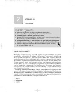
As its name suggests, this considers how difficult items are and how difficult it is to get them right. It is sometimes also referred to as ‘item facility’ in item response theory, which looks at the same thing but from the opposite view, i.e. item easiness. The difficulty indicator, known as the p value, represents the percentage of participants who have answered an item correctly and is calculated by dividing the number of people getting it right by the total number who attempted it. Clearly, if everyone got it right then the p value comes out as value 1.0, while if no one got it right then the p value is 0, so that the p values for all of the items will range from 0 to 1. A high value suggests most people answered correctly and, therefore, the item may be too easy. If everyone gets it right, then it simply increases all scores by 1. In this case, where an interval scale is used, the item will have no effect. On the other hand, a very low value suggests few got it right and that the item may be too difficult. If everyone gets an item wrong it will not make any contribution to the total scores and is redundant. If all is well, the mean item p value is about 0.50, indicating a moderate difficulty level. Very high or low values tend not to discriminate effectively between people so items having extreme values need discarding or re-designing. This approach provides useful information for the design of ability, aptitude or achievement measures. But it does not mean that a mean p value of 0.50 is always appropriate because a high level assessment of cognitive ability may need more difficult items and, therefore, a lower mean value. It also does not work well when the items are all highly inter-correlated, because in this case the same 50 per cent of candidates will pass all of the items and just one item will suffice to differentiate groups. The way out of this is to create items of varying difficulty, providing a balance between easy and more difficult ones, and ensuring an average p value of 0.50. In some instances tests are designed to start with easy items and to get progressively more difficult. This is useful in assessment of individuals, such as for clinical measures, so that an assessor can identify where the person’s cut-off is for successful responses and does not have to administer the whole test. The WAIS tells you how to do this by stating a discontinue rule, for example to stop after three consecutive scores of 0. Analysis of difficulty can also be used to check whether any item exhibits bias or unfairness. If there is a different pattern of responses for one group compared to another, this may suggest the items concerned are not measuring the same construct for both groups and may unfairly discriminate. For example, we might give a test having just eight items to two groups and then rank the items in terms of the percentage of correct responses made by each group (the percentage ranks decreasing from 1 to 8), as shown in Figure 2.1. Seven of the items tend to show a generally similar pattern for both groups and the differences vary only by random fluctuations of one or two points. But item 3 appears to be rather harder for the second group, with a much smaller percentage of people answering correctly. Therefore, it appears harder for • 38 •


30/07/2009

8:05 PM

Page 39


Group 1 Rank Group 2 Rank Difference

Item 1

Item 2

Item 3

Item 4

Item 5

Item 6

Item 7

Item 8

1 2 −1

2 1 1

3 8 −5

4 3 1

5 6 −1

6 4 2

7 5 2

8 7 1

Figure 2.1 An item difficulty approach to identifying unfairness

members of group 2 than for group 1. It may have inappropriate language or meaning for group 2 or it requires knowledge which its members are less likely to possess.

Item discrimination analysis

This evaluates whether a response to any one item is related to responses on all of the others. It identifies which are most effectively measuring the characteristic under investigation and whether they are distinguishing between those people who do well and those who don’t. It checks that those who perform well on the measure overall are likely to get a particular item right, while those doing poorly overall are going to get it wrong. Imagine the case of an item which turns out to be answered wrongly by people who get a high total score but correctly by those gaining low scores overall. There is something clearly odd here because it seems to have a negative discrimination. More often it is found that an item has zero discrimination, suggesting that people having low scores overall are as likely to answer correctly as those who do much better. Therefore, the item is, perhaps, measuring something completely different from all of the others. One way of investigating discrimination involves comparing high scorers and low scorers. The discrimination index d then compares the number of high scorers who answered an item correctly with the number of low scorers who also got it right. If the item is discriminating effectively between these groups, then more of the high scorers should get it right compared to the low scorers. The groups can be fixed by comparing the top and bottom quarters or thirds – the most appropriate percentage recommended for creating these is the top and bottom 27 per cent of the distribution of scores. If Ph and Pl are the numbers of people getting the item right in the higher and lower scoring groups, and Nh and Nl are the number of people in these groups, then d is calculated using the equation: d = Ph Nh

−

Pl Nl

Items which discriminate well, being harder for the lower scoring group and easier for the higher group, have large, positive values of d. Those having a negative value are going to be easier for those who do less well, and are candidates for removal.

Analysis of item – total correlations

A popular method for evaluating how well an item can discriminate lies in calculating the correlation between it and a total score on the measure, which is used in test • 39 •


30/07/2009

8:05 PM

Page 40


construction as we shall see in Chapter 3. The relationships between how individuals responded to each item are correlated with the corrected total score on the measure (Guilford and Fruchter, 1978). The correction is made to ensure that the total score does not include the response to the item being evaluated as total scores containing that item will have a spuriously higher relationship than total scores made up of only the others. This correction is important when there are only a few items. The underlying question addressed by each correlation coefficient is: How do responses to an item relate to the total test score? Those items having high positive item-total score correlations are more clearly related to the characteristic being measured. They also have greater variability than other items with low correlations, suggesting they will discriminate more between high and low values. A negative value will indicate that an item is negatively related to other items. These are not useful because most measures try to assess a single construct and, therefore, you would expect them to have a positive correlation. Those having low correlations indicate that they do not fit in and need to be improved, omitted or replaced (Nunnally, 1978). Publishers sometimes show tables of these correlations in their manuals.

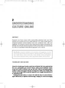
Item Response Theory (IRT) This is the name given to a range of models designed to investigate the relationship between a person’s response to an item and the attribute being measured, often described as an underlying ‘latent trait’. In fact, the theory has also been called ‘latent trait theory’ (Birnbaum, 1968; Hattie, 1985). Whatever we call it, the theory can provide a wide-ranging analysis of items. It was originally developed to overcome problems with CTT. All of its models have in common the use of a mathematical function to specify the relationship between observable test performance and an unobservable trait. Because of this the approach has become highly mathematical, provoking debate about its focus upon this and its effectiveness in actually helping to make psychological measures. Basically, it aims to analyse the relationship between responses to items and the associated trait, explaining how individual differences influence the behaviour of the person responding. Imagine someone taking a test of, say, diagrammatic reasoning, then it would make sense that a person who has a high capacity for this is more likely to get a difficult question right and, the opposite also, that a person of low ability would be more likely to get it wrong. So how someone responds to items is linked to the amount of attribute possessed by the person. This can be demonstrated graphically, as shown in Figure 2.2, which has the level of the attribute (or the total test scores obtained) along the horizontal x-axis and the probability of getting an item right on the vertical or y-axis. Different test items will usually have different difficulty levels, as shown by the curves for three items. IRT is based on this form of graph which relates the probability of answering correctly, for each item, to a respondent’s ability. Each item has its own curve. If what we have said above does make sense about items then, if an item is assessing the attribute, the probability of getting the correct answer should increase as the level of the attribute • 40 •


30/07/2009

8:05 PM

Page 41


Item 1

Probability of Correct Response

Item 2 Item 3

Level of Attribute Figure 2.2

Item-characteristic curves for three hypothetical items

increases, so the graph needs to rise on the right-hand side. If it doesn’t, there must be something wrong. Mind you, if an item is not actually measuring what it is intended to measure, i.e. is not valid, then even high-level individuals may not answer it correctly and so a probability of 1.0 or 100 per cent may not be achieved. Even good values of the difficulty and discrimination indices can provide no certainty that any one item is working effectively. As the level of the underlying attribute increases, the probability of answering correctly should increase. For an item to be difficult it needs a large amount of the attribute to be able to get it right. A slightly different way of plotting this graph would be to plot the total test scores of individuals (as a measure of performance) along the x-axis against the proportion of people who gave correct responses to a particular item on the y-axis, meaning that we are looking at correct performance on this item relative to ability. The same sort of graph should result, all being well, of course. This kind of graph enables us to determine whether an item is behaving in the right kind of way, and is known as an item characteristic curve (ICC) (Lord, 1974, 1980). By looking at it we can work out item difficulty, discrimination and even the probability of responding correctly by guessing. Item difficulty can be seen by examining the curve. With a difficult item, the curve needs to start to rise on the right-hand side. Easy items will have the curve beginning to rise on the left-hand side. If an item crosses the 0.5 probability level well to the left, then it is easy and respondents of moderate ability have a high probability of getting it right. But if the curve crosses the 0.5 probability point further over to the right, then it must represent a more difficult item. The difficulty level is the score at which • 41 •


30/07/2009

8:05 PM

Page 42


50 per cent of respondents give the correct answer. Item discrimination can be evaluated by inspecting the slope of the curve. The flatter the curve, the less it will discriminate between people – those with lowest discrimination will be flat. The discrimination index is the slope or gradient of the curve at the 50 per cent point. A small value suggests that people with a broad range of abilities have a reasonable chance of getting the item right. A high value will tend to make the curve become more upright. However, someone who is low on the attribute may try to guess the answer rather than attempt to work it out. If the item is easy to guess then more people of low ability are likely to get it right (when they shouldn’t), and the graph hits the y-axis higher up, i.e. the higher the curve starts on the y-axis the higher the chance of guessing correctly. In Figure 2.2 items 2 and 3 are easier than item 1 because their curves begin to increase further left. Item 3 is the least discriminating because its curve is flatter. Item 3 is also most vulnerable to guessing because it starts from a position higher on the y-axis. The two indexes of item difficulty and discrimination are similar to those obtained by classical analysis, although the ICC gives a more detailed understanding of how items function. When items vary only in terms of their difficulty, the curves run parallel to each other, with the more difficult items closer to the right-hand side, and this is referred to as a one-parameter model, only involving the difficulty variable. The assumptions made in using the curves are, firstly, that the probability of an individual answering an item correctly depends upon ability and the difficulty of the item, and is not associated with responses to other items and, secondly, that all of the items included measure only one attribute. The ICC graphs can be described by a mathematical equation known as the logistic function (Weiss and Yoes, 1991) which ensures that the probability of a person answering correctly cannot have values outside of the range from 0 to 1.0 and that the curve moves upwards at a point set by the level of difficulty. The one-parameter logistic function described enables a test designer to determine the probability of any individual passing any item based upon knowledge of the person’s ability and item difficulty (Rasch, 1980; Mislevy, 1982). Other models are based upon increasing the number of parameters involved. When both difficulty and discrimination factors are taken into account, unsurprisingly, the formula for a two-parameter function is needed. Introducing an allowance for guessing results in a three-parameter function. Employing computer programmes to do the calculations, IRT aims to determine the most likely values for these parameters and the person’s performance on the attribute independently of the actual difficulty of items and of the sample (Hambleton and Swaminathan, 1985). This is different to classical theory, where an individual’s score is seen as the measure of the attribute and is linked to the difficulty of items. To do this IRT evaluates the fundamental algebraic characteristics of the ICC curves so as to extract equations which can predict the curve from basic data. Computer programs have been designed such that their estimates of these parameters are close to their true values for the one- and two-parameter models, provided that the number of items and individuals are large. An example of a one-parameter model for analysis, using item difficulty only, is known as the Rasch model, based upon the name of its original designer (Rasch, 1960, • 42 •


30/07/2009

8:05 PM

Page 43


1966), and some researchers have developed this as an alternative approach to IRT known as Rasch Scaling. The mathematically oriented Rasch model assumes that indices for guessing and item discrimination are negligible. It also assumes, quite obviously, that the higher the individual is on the latent trait and the easier the item concerned, then the more likely it is that the person will answer correctly. Items in a particular data set are thought internally consistent and homogeneous if they conform to the model. Being mathematically similar to IRT, it is designed to help with the construction of stable linear measures, while IRT is used to find the statistical model which best accounts for observed data. A relevant domain for the use of the Rasch model might be in assessment situations involving large populations. Its problems, however, are complex and have been the subject of much debate (Levy, 1973; Barrett and Kline, 1981; Roskam, 1985) including the suggestion that some of its assumptions are wrong. The two- and three-parameter models have been less subject to criticism and, with the development of computer sophistication, have gained in usefulness.

Comparing Classical Test Theory and Item Response Theory Item analysis literature suggests that each of the theories has its own devotees, although both have advantages and disadvantages. Being the most longstanding approach, CTT is often referred to as a ‘weak model’ because its assumptions are easily met by traditional procedures (Kline, 2000). Although its focus is on test-level information, item statistics including difficulty and discrimination are also important. At this level the theory is relatively simple, since there are no complex models to understand. Major benefits include that fact that analyses can be carried out using smaller representative samples, that it makes use of relatively simpler mathematical procedures and that the estimations of parameters are more straightforward. Its theoretical assumptions make CTT easy to apply in many testing situations. However, it has several important limitations, including the problem of the item difficulty and discrimination parameters being both sample dependent. Another concerns the assumption that errors of measurement are the same for all respondents and are, therefore, constant across the trait range. In contrast IRT models are generally referred to as ‘strong’, since the associated assumptions may be difficult to meet with test data. IRT is more precise than classical theory and its precision can develop more accurate methods of selecting items. Because of these benefits the theory has gained increasing attention in test design, item selection, in dealing with bias and in evaluating scores. But beware: the literature on IRT is highly technical. Its models are mostly designed to assess intellectual functioning and need large samples. Despite its advantages, many of its models assume that constructs are unidimensional and this is a problem in assessing personality as some of its constructs are inherently multidimensional (Wood, 1976). IRT should result in samplefree measurements and publishers would like this because having fewer samples to collect means a less expensive validation process! Empirical comparisons of the two approaches have suggested, funnily enough, that their outcomes are not much different, • 43 •


30/07/2009

8:05 PM

Page 44


especially when large data samples have been used (Fan, 1998). Integration of both approaches is probably key to the future development of assessment methods.

Summary How items are constructed depends upon the kind of psychological assessment intended and a range of different methods are available for this. A unidimensional measure focuses upon the assessment of only one attribute. Two principal approaches have been applied to understand the effectiveness of items: Classical Item Analysis, based upon Classical Test Theory (CTT), and Item Response Theory (IRT). CTT’s principal focus is upon both test-level information and item statistics, and it is viewed as a ‘weak model’ because its assumptions can be easily met by traditional psychometric procedures. Based upon Item Characteristic Curves, IRT employs mathematical models to understand the behaviour of items, and is a ‘strong model’ in that its assumptions may be more difficult to meet in analysis of test data. Mathematical equations have been applied for one-, two- and three-parameter logistic functions.

Measuring Attitudes One area of psychological practice which involves the development and use of measurement scales is the study of attitudes. Attitudes are abstract hypothetical constructs which represent underlying tendencies of individuals to respond in certain ways, and they can’t be measured directly. The term ‘attitudes’ is useful in two ways: first, when we want to explain someone’s past or present behaviour towards others, or an issue, object or event, and secondly when we try to predict how the person will behave in the future. If we observe that an individual avoids certain other people, frequently makes disparaging remarks about them, and visibly bristles when someone enters the room, then we attribute to the person a particular form of negative attitude. An attitude is, therefore, an attribution made towards something, someone or some event. We identify it when an individual behaves consistently across many situations, encouraging us to make the attribution. Other factors may be associated in order to characterize it, for example its importance, focus, intensity or magnitude, and the person’s feelings which contribute to these may be positive or negative. In seeking to measure an attitude we are concerned with its magnitude and direction. There have been many attempts to define the term. The most well-known is that of the social psychologist Gordon Allport who said, ‘An attitude is a mental and neural state of readiness, organised through experience, exerting a directive or dynamic influence upon the individual’s response to all objects and situations with which it is related’ (cited in Gahagan, 1987). Others have viewed it as a tendency to evaluate a stimulus (whatever that is) with some degree of favour or disfavour, being expressed in cognitive, emotional or behavioural responses (Ajzen and Fishbein, 2000). The common view is that an attitude is a predisposition to behave in a particular way and its • 44 •


30/07/2009

8:05 PM

Page 45


‘object’ may be anything a person distinguishes from others or holds in mind, whether concrete or abstract. Attitudes change as people learn to associate them with pleasant or unpleasant circumstances or outcomes. Measurement of attitudes is an important part of applied psychology because it is so widely used, for example a clinical neuropsychologist may want to assess the attitudes of a patient’s family towards rehabilitation and support services offered, just as a clinical psychologist might want to know the views of carers about their service, too. Similarly, a forensic psychologist might be interested in understanding the attitudes of other prison service employees. An occupational psychologist might be interested in knowing the attitudes of employees towards proposed changes in the workplace. Attitudes influence how people behave and, therefore, may deter or ensure support for services at many professional levels, whether individual, group or community. Disregarding people’s attitudes can hinder collaborative working in many settings, whilst knowledge about them can guide service development and facilitate planning and change.

Attitude Measurement To make inferences about the attitudes of any group we need data from its members. One way of doing this might be to make direct observations. This might be possible in some situations, for example in dealing with small groups or with children, although the accumulation of data will often be time-consuming and possibly expensive. Another approach might be to ask people directly what their attitudes are, although the trouble with this again is that it would be rather unscientific and have no means of accurate measurement. A number of measurement techniques, mostly using questionnaires, have been developed for the analysis of attitudes. Different scales have also been developed. Construction of attitude questionnaires shares similar characteristics to those we have discussed in relation to other psychological attributes: we must firstly design items which are relevant and appropriate and then make use of a scale representing different numerical values. The most common method used has been to develop a scale made up of a set of positive and negative statements.

Thurstone’s Scales Thurstone and his colleagues used two approaches to the development of attitude scales in 1929: pair comparisons and equal-appearing intervals (Thurstone and Chave, 1929; Thurstone, 1938). First, they collected a large number of items indicating both positive and negative thoughts about a particular topic. The pair comparisons method was more difficult and time-consuming because it involved asking many people referred to as ‘judges’ to compare the items with each other and to identify which one in each pair indicated the more positive attitude. The method of equal-appearing intervals has been more widely used because, instead, the judges are asked to independently sort items into 11 categories on a continuum • 45 •


30/07/2009

8:05 PM

Page 46


ranging from most favourable, through neutral, to the most unfavourable attitude. In some instances the favourable to unfavourable dimension may not apply and an alternative dimension based on a degree of attitude needed. The 11 sets of items are designed to be placed at equal intervals along this continuum, so that the difference between any two adjacent points is identical to that between any other two points. Positions on the scale of the different items are then identified solely on the basis of how favourable or unfavourable they are. One way of doing this might be for each item to be written on a card so that they can be more easily sorted into 11 groups. A frequency distribution can be constructed for each item based on the number of experts who located the item in each category, enabling the scale value or median to be determined. Scale values could then be used to rank order items and to determine the items selected (usually about 20 to 40 in number). This means that, when complete, every item in the Thurstone scale has a pre-determined numerical value. Any individual’s score on the scale is the mean of the values of the items chosen. One problem with this method of attitude measurement involves the fact that two respondents could end up with the same score from quite different patterns of responses. A second is that the sorting of items by the judges may be associated with their own subjective opinions, rather than being neutral (Bruvold, 1975), although Thurstone thought they would sort objectively and not be affected by personal views. It was thought possible to instruct the judges to limit any judgemental bias. Lastly, although Thurstone had tried to construct a technique leading to an objective equalinterval scale, it seems that in reality the scale is an ordinal one. Objections raised to this approach have concerned both practical and theoretical issues. The practical disadvantage suggests that for the scales to have accuracy 100 judges are needed and that these should be representative of the population for which the test is intended (Edwards, 1957). Theoretical objections involve the view that Thurstone scales are not consistent with the structure of attitudes and on these grounds their use is not recommended (Nunnally, 1978).

Likert Scales If you want to design an attitude scale quickly, then the Likert scale approach is the one for you, because it has the advantage of not needing the judges (Selltiz, Wrightsman and Cook, 1976). This is based on the work of Rensis Likert (1932) and many researchers prefer his method. To construct Likert scales a large number of favourable and unfavourable items need to be developed. This time, however, they are administered to a large trial group of respondents who rate them on a continuum, often from 1 through to 5, sometimes from 1 to 7. In the use of the five-point scale the numbers are given meaning, usually 1 = strongly agree, 2 = agree, 3 = not certain or undecided, 4 = disagree and 5 = strongly disagree. Total scores on this initial set of statements are determined by summing the scores for all of the items. From the total scores a discrimination index can be calculated, enabling selection for the final questionnaire of positively and negatively phrased items which discriminate significantly between respondents. Only those statements, therefore, are • 46 •


30/07/2009

8:05 PM

Page 47


used which best differentiate between high and low scorers. Item analysis is also conducted to establish whether they are all measuring the same attitude. However, people sometimes make questionnaires which look like a Likert scale but have not subjected their statements to item analysis like this, as he suggested. It is not always possible to tell whether something is really a scale which has been designed using the Likert method. The scale is also referred to as the scale of summated ratings because any individual’s attitude score is the sum of all of the ratings for the different items in the questionnaire. Compared to the Thurstone scale, it does not involve a panel of judges and respondents indicate a level of agreement or disagreement towards items. But it, too, is ordinal and so can only order the attitudes of individuals on a continuous dimension, being unable to determine the magnitude of differences between scores. It is also similar to the Thurstone scale in that different patterns of responses may provide the same total score. The major advantages are that the scale is easier and quicker to construct, it allows the use of a diverse range of items provided they are significantly correlated with total scores, and it tends to have greater accuracy than the same number of items in the Thurstone scale (Cronbach, 1946; Selltiz et al., 1976). This has led to the existence of many modern attitude scales based on the Likert model. But the approach assumes a linear model, i.e. that the sum of item scores has a linear relationship with the attribute measured, and it should, therefore, be considered with measures constructed on the basis of Classical Test Theory. This means Likert scales have all of the psychometric advantages of CTT measures, for example the more steps there are in a rating scale, the more reliable it is (see Chapter 5 for discussion of reliability). With Likert scales reliability increases up to the point of seven steps and then becomes level.

Guttman’s Scalogram Unidimensionality was mentioned earlier. We said that for any assessment to be a good measure of an attribute it needs appropriate items to match and a scale which measures only that and nothing else. Louis Guttman sought in the 1940s to develop a method which would identify whether responses on an attitude questionnaire represent a single dimension and thus reflect unidimensional attitudes (Guttman, 1944). His method is less well-known than those of Thurstone and Likert. Using his scalogram analysis Guttman arranged his items in increasing order of difficulty of being accepted by respondents so that if an individual agrees with an item which states a higher level of acceptance then that person must agree with all the other items at a lower level. This would work only if all of the items in the scale are representative of the same attitude in the same way as cognitive test items which are measuring the same construct. The aim of the scalogram is, therefore, the design of a cumulative ordinal scale. Guttman thought that, despite the difficulty of establishing a true interval scale, his approach could make an approximation to this. A factor called the reproducibility coefficient could be determined to indicate the degree to which a true unidimensional scale is derived and this is determined by calculating the proportion of • 47 •


30/07/2009

8:05 PM

Page 48


respondents whose responses fit into a perfect arrangement having an increasing degree of acceptance. Construction of the scalogram involves the collection and arrangement of items in such an order that people would accept the first and, proceeding through the list, reducing numbers of people would endorse subsequent ones. They are presented to a large sample of people to determine the increasing degree of acceptance. The statements are then modified, arranged and administered again, with the process being repeated until a set of items is developed which demonstrates the increasing acceptance. The final outcome is the scalogram, having items identified by empirical analysis which can then be used to measure the attitudes of others. Any individual’s score on the questionnaire is the total number of successive or nearly successive items endorsed. The difficulty in practice, however, is that often people will omit items, indicating the complexity of human attitudes, and that a perfectly unidimensional scale is not easy to construct. The perfect ordering of items suggested by Guttman appears to have an intuitive appeal (Nunnally, 1978), especially in view of the fact that length, volume and weight can form perfect Guttman scales. However, modern psychometric analyses have shown also that, like one-parameter Rasch scaling, the underlying model of Guttman scaling does not fit well with psychological theories and it is unlikely that items could correlate perfectly with total scores on any particular measure (Kline, 2000). This means that perfect unidimensionality can’t be achieved. And the scales are based on ordinal measurement only.

The Semantic Differential The Semantic Differential, also a type of numerical rating scale, was developed by Osgood, Suci and Tannenbaum (1957) following studies in a range of cultures. It has been used extensively in research in the fields of personality and social psychology. Their research suggested that people give meaning to terms and concepts with regard to three dominant aspects, known as semantic dimensions. These are: • The Evaluative Dimension: Good – Bad • The Potency Dimension: Strong – Weak • The Activity Dimension: Active – Passive Their semantic differential was designed to provide a measurement based upon the meanings people attribute to terms or concepts connected with attitudes. This uses a questionnaire which lists bipolar adjectives such as good–bad, valuable–worthless, enjoyable–unenjoyable or friendly–unfriendly. Each bipolar pair is linked to a dimension or scale having seven points with the two ends represented by the contrasting adjectives, and the mid-point being a neutral position, like this: Good Valuable Enjoyable Friendly

1 1 1 1

2 2 2 2

3 3 3 3

4 4 4 4 • 48 •

5 5 5 5

6 6 6 6

7 7 7 7

Bad Worthless Unenjoyable Unfriendly


30/07/2009

8:05 PM

Page 49


Osgood et al. devised scales like these in order to study the connotative (personal) meanings that concepts such as ‘sickness’, ‘sin’, ‘hatred’ and ‘love’ generate among people. These concepts could then be extended to others which generate attitudes, for example ‘sport’, ‘politics’, ‘television’ and so on. Obviously, the choice of bipolar adjectives depends on the concept being investigated. Many of these will be evaluative and will principally indicate a person’s feelings about it. The number of points across the scales can also be varied. Respondents asked to complete the measure will simply be asked to make a mark on the scale points which indicate their attitude. It has been found that even young children, who would have difficulty with Thurstone or Likert scales, are able to respond to the semantic differential (Gahagan, 1987). A person’s overall attitude score is represented by the sum, or possibly the mean, of the scores marked on all the dimensions. The responses to each concept may also be scored on the semantic dimensions (evaluative, potency and activity) and, by comparing these for one construct or more, to gain understanding of what is called the person’s ‘semantic space’. However, responses which fall at the centre of the scale may be difficult to interpret, possibly representing either indifference or ignorance, and further investigation may then be needed to establish the person’s view. In some instances it may also be possible that the individual responds by marking the extreme ends of the scale throughout the measure, regardless of any attitude adopted. This might not become clear unless a number of measures are administered.

Limitations of Attitude Measures One problem common to all of these attitude measures is that of social desirability. This means that people may respond to them in a manner which has been influenced by the investigator or to preserve their self-image in some way. People could also feel apprehensive about disclosing their true attitudes towards an issue. Some may adopt what is called a ‘response set’, that is, they may adopt a consistent tendency to agree or disagree with statements, regardless of their meaning. Tactics have been adopted by designers to overcome these problems, for example in trying to make a measure’s purpose less obvious by including irrelevant items and by giving assurances about anonymity and confidentiality. An individual’s response set may also be disrupted by the inclusion of both positively and negatively expressed items. A multi-indicator approach to attitude measurement, involving administration of a number of instruments, is probably the best way of providing more reliable and valid assessments, and acknowledges that people’s attitudes are more complex than previously thought. Attitudes were once perceived to be simple in nature and more straightforward to measure. Today this has changed to reflect the view that they are more interconnected and multifaceted than once thought.

Summary In this section we have explored attitudes, how they are defined and how they can be measured. Key factors are that they tend to be consistent, are related to a person’s • 49 •


30/07/2009

8:05 PM

Page 50


feelings, and have importance, focus and intensity for the individual. Although they have been defined in different ways, they are thought to represent predispositions to behave in particular ways towards some stimulus. A number of measurement techniques and scales have been developed for their assessment including Thurstone’s and Likert’s scales, Guttman’s Scalogram and the Semantic Differential. This chapter has focussed upon the two things said to be the basic components of psychological assessment and measurement, i.e. scales and items. We have seen how different types of item can be constructed and that, through the use of scaling, the responses of individuals can be transformed into quantitative measurements. We have also seen how analysis can be made of the effectiveness of the items which go to make up a measure, including such aspects as their difficulty and their discrimination between responses. Analytical approaches have advanced substantially over the years, especially through development of computer technology and mathematical modelling. The specific applications of measurement techniques to the study of attitudes have also been examined. We have learned: • The different types of scale and items available for scientific measurement and how they may be most effectively applied to assessment. • The key principles of approaches to item analysis, such as Classical Test Theory and Item Response Theory, and their advantages and limitations. • About the nature of attitudes and their measurement, including the different approaches of Thurstone, Likert and Guttman, and the Semantic Differential.

• 50 •

Chapter Two

Chapter Two

Suggest Documents

Chapter two

Chapter two

CHAPTER TWO

Chapter Two

Chapter Two

CHAPTER TWO

Chapter Two

Chapter Two

CHAPTER TWO - Gericom

CHAPTER TWO - Gericom

Chapter Two - Sage Publications

CHAPTER TWO: RESEARCH APPROACH

chapter two - Plant Physiology

Chapter Two Related Work

Chapter Two - Sage Publications

Chapter Two - Free Ebooks

chapter two: method

Chapter two Literature Review

CHAPTER TWO Load Estimation

Chapter Two - Sage

Chapter Two - Google Sites

chapter two

CHAPTER TWO - Gericom

chapter two - AgEcon Search