We obtain a network traffic model for real-time MPEG-II encoded digital video by ... To achieve high multiplexing efficiency we propose a traffic shaping scheme ...
Characterization, adaptive traffic shaping and multiplexing of real-time MPEG-II video Sanjay K Agrawal, Charles F. Barry, Vinay Bannai (NUKO Systems), and Leonid Kazovsky Stanford University, Department of Electrical Engineering Durand Bldg, Rm. 202, MC9515 Stanford, CA 94305 BroadBand Networks Corporation 990 Richard Avenue, Suite 112 Santa Clara, California 95050
ABSTRACT We obtain a network traffic model for real-time MPEG-II encoded digital video by analyzing video stream samples from real-time encoders from NUKO Information Systems1. MPEG-II sample streams include a resolution intensive movie, City of Joy, an action intensive movie, Aliens, a luminance intensive (black and white) movie, Road To Utopia, and a chrominance intensive (color) movie, Dick Tracy. From our analysis we obtain a heuristic model for the encoded video traffic, which uses a 15-stage Markov process to model the I, B, P frame sequences within a Group of Pictures (GOP). A jointly correlated Gaussian process is used to model the individual frame sizes. Scene change arrivals are modeled according to a Gamma process. Simulations show that our MPEG-II traffic model generates I, B, P frame sequences and frame sizes that closely match the sample MPEG-II stream traffic characteristics as they relate to latency and buffer occupancy in network queues. To achieve high multiplexing efficiency we propose a traffic shaping scheme which sets preferred I-frame generation times among a group of encoders so as to minimize the overall variation in total offered traffic while still allowing the individual encoders to react to scene changes. Simulations show that our scheme results in multiplexing gains of up to 10% enabling us to multiplex twenty 6Mbps MPEG-II video streams instead of 18 streams over an ATM/SONET OC3 link without latency or cell loss penalty.
Keywords: Real-time MPEG-II, Encoder Feedback, Statistical Characterization, Traffic Shaping, ATM Multiplexing
1. INTRODUCTION Broadcast-quality MPEG-II digital video has already proliferated in telecommunications, cable and satellite broadcast domains. In the near future the demand for MPEG-II will likely explode in desktop domains for interactive applications. In these domains, Asynchronous Transfer Mode (ATM) has gained much attention because of its effectiveness at multiplexing voice, video and data together. Yet to efficiently transmit and multiplex variable bit rate (VBR) MPEG-II traffic in packet-switched ATM networks while still providing Quality of Service (QoS) guarantees is not a trivial task. Real-time MPEGII sources offer a unique challenge to network transport because of the combined requirements of lowlatency, low-loss over widely varying data rates. In this paper, we are chiefly concerned with our ability to predict the required source and network resources, which allow us to meet the QoS targets while maximizing the number of simultaneous connections on the network. Ultimately, we would like not only the network to react to the varying 1
The products used along with all intellectual property and patents pending derived from this white paper are the sole property of BroadBand Networks Corporation.
1
bandwidth demands of the encoding process, but for the encoding process to react to the availability of network bandwidth. By “closing the loop” between the network and encoder, we can expect to have some gains in terms of the number of simultaneous MPEG-II processes while maintaining QoS requirements such as low-latency and low packet loss.
2. DESCRIPTION OF THE REAL-TIME MPEG-II PROCESS We now turn to the description of the real-time MPEG-II process as it relates to transport in networks2. First, real-time MPEG-II encoders generate 30 frames of encoded video per second. Depending upon the spatial and temporal redundancy in a frame and between consecutive frames the encoder selects one of three basic types of encoding schemes (frame types). Interpolative I-frames are based on only the current video frame and rely only on spatial redundancy to achieve compression. Bi-directional B-frames take advantage of both spatial and temporal redundancy between past, current and subsequent video frames to achieve higher compression (small frame size) and much less variability in size than I-frames. Predictive P-frames also compress spatial and temporal redundancy between current and subsequent frames. Pframes are intermediate in size and variability. A typical MPEG-II process yields frame sizes, which may vary from 100KB (large I-frame) to 8KB (small B-frame). This variability places extreme demands on the network. If we can predict the sequence and size distribution of B, P frames, and I then we can more efficiently allocate network resources. To this end, we note that MPEG-II defines the allowable sequences of I, B, and P frames within a larger framework called the Group of Pictures (GOP). Specifically, the NUKO encoders, which use the C-Cube chipset, typically generate a 15-frame GOP with the sequence IBBPBBPBBPBBPBB. Shorter, truncated GOPs are allowed in certain situations such as scene changes, e.g., IBBPBB, IBB, etc. The selection of the encoding sequence is a tradeoff between latency, compression and error propagation. Conceptually it is clear that B- and P-frames are preferred to I-frames in terms of reducing the overall data rate for compressed video. However, At least two things conspire to make I-frames necessary. The first is the need to limit error-propagation. That is to say there are certain classes of errors (missing or errored data packets), which cause propagation of errored pixels from frame to frame by the MPEG-II decoder. In these cases, the only way to terminate the propagation is with an I-frame because I-frames can be decoded without reference to any other frames. Thus, typical real-time encoding systems limit the maximum length of the GOP. Specifically, the NUKO encoders limit the maximum GOP to 15 frames (1/2 second). The second need for I-frames occurs when the video source abruptly changes its content, i.e., a "scenechange". I-frames are more suited to scene changes because they set the context for subsequent B-frames. This is analogous to flushing and re-filling of a cache in computer systems. When a scene change occurs, the encoder reacts by terminating the current GOP and starting a new GOP with a new I-frame. Thus a GOP can be less than 15 frames when reacting to scene changes. An additional key feature of real-time MPEG-II encoders is their capability to regulate the average bandwidth over the entire GOP. In other words, although the individual frame size and bandwidth of any frame type can vary over a wide range, the total bandwidth over a GOP can be maintained very closely to a preset long-term average. This represents a tradeoff between constant bit rate (CBR) and constant quality video. In the case of the NUKO encoders, the long-term average can be selected anywhere from 3Mbps to 25Mbps. For all the samples and analysis in this paper, 6Mbps was used as the long-term average bit rate. Although the mechanisms that actual real-time encoders use to generate the I, B, P sequences, to detect scene changes and to maintain average bit rate are beyond the scope of this paper, we have presented enough to make a significant observation. If the scene change inter-arrival time is greater than 15 frames, then it should be possible to predict the encoded frame type quite accurately for not only several frames in advance but perhaps over an entire GOP (up to 500ms). In addition, if the distribution of the expected
2
We assume NTSC, CCIR601 quality video sources.
2
frame sizes for each frame type is known then it is then possible to negotiate and allocate ATM network resources based on these predictions.
From the standpoint of multiplexing many concurrent real-time streams we make the following observations. First, each real-time MPEG-II encoder generates frames in a quasi-static fashion, i.e., frames are generated every 30th of a second. Moreover, the variation in arrival time from frame to frame is minimal (20-40 ppm for typical video systems). Therefore, based on tracking each encoder’s GOP sequence, it is possible to accurately predict which encoders will generate which types of frames and therefore predict the sum total required network bandwidth. The trick is to allocate enough bandwidth to each process such that each source sees a minimal packet loss QoS while not impacting the packet loss QoS of the other encoders. These QoS guarantees can be achieved deterministically or statistically. Deterministic guarantees require ample network resources, while statistical guarantees achieve high network utilization at the cost of occasional packet loss and network delay [1,2]. In the simplest deterministic case, each encoder is granted a guaranteed bandwidth in excess of the average long-term rate. This guaranteed bandwidth is chosen such that the likelihood of packet loss is less than 1 packet in 1012. For example, 18 such 6Mbps sources can be multiplexed onto an ATM OC-3 link, each source being allocated 7.5 Mbps. In this case, the ATM multiplexer is 80% utilized. On the other hand, statistical guarantees use statistical multiplexing which necessitate statistical characterization and modeling. If we can accurately predict the requirements of each encoder in advance, and even more so, to modify the encoder behavior to better suit the network, we can expect to achieve a higher multiplexer utilization. Following our characterization of MPEG-II traffic, we present one such scheme that improves multiplexer efficiency by up to 10%.
3. TRAFFIC CHARACTERIZATION To characterize the real-time MPEG-II processes, we sampled and analyzed several different types of video. Our analysis is based on several large and complete video samples obtained using NUKO Information Systems encoders, which use C-CubeTM’s MPEG-II algorithm. Each sample comprises 2.2 Gigabytes of data from 44-minute long video sequences from several different types of video broadcasts: (a) the resolution intensive movie Blade Runner; (b) the action intensive movie Alien; (c) the luminance intensive (black and white) movie Road To Utopia; and (d) the chrominance intensive (color) movie Dick Tracy. In modeling the MPEG-II process we focused on those aspects that are most appropriate from the standpoint of multiplexing several simultaneous sources over and ATM network. In particular, the fastest reaction time in ATM networks, from request to allocation, is tens of milliseconds and more commonly, hundreds of milliseconds. For this reason, we limited the granularity of our approach to frames (33ms) and GOPs (up to 500ms) rather than smaller increments such as slices or macroblocks. In addition to focusing on network related aspects, we chose to develop a heuristic model based on observations of the empirical data. The strength of a heuristic approach is that we can relate our parameters to the intuitive behavior of video (i.e., content and scene changes) and that we can also relate it to the underlying MPEGII algorithm software unlike few frame based approaches [7]. Many other approaches to MPEG modeling have been reported in the literature based on schemes such as linear adaptive prediction [2], TES modeling [4,6] which we view as highly non-intuitive. Other schemes are based on time frames too small to be of interest in ATM wide area networks [5]. A disadvantage of our heuristic approach is that we cannot know how well it can be applied to other types of real-time MPEG-II algorithms from vendors such as CLI and IBM. In the following, we develop our model in the context of the NUKO encoders. Figure 1 shows a 1000-frame (33.37 second) sequence of I, B, P frames from the movie Dick Tracy. From the figure we immediately see that the overall process maintains an average bandwidth (25KB/frame; 6 Mbps), and each of the I, B, and P processes have their own average bandwidths and variations about that
3
average. I-frames, for instance, average about twice the overall average size, or some 51 KB (12.24Mbps). In addition, I-frames are widely varying-from 27KB to over 84 KB (6.48 to 19.92 Mbps). P-frames average little less varying than I-frames, averaging 34KB (8.16 Mbps). P-frames vary from 18 KB to 38KB (4.32Mbps to 9.12Mbps). B-frames are the best behaved, averaging just 18KB (4.32Mbps) and varying from 8KB to 24KB (1.92Mbps to 5.76Mbps). From these observations, it is obvious that nearly all I-frames and most P-frames will result in filling of source buffers in a flow-controlled ATM environment (e.g., if the leaky-bucket is used). On the other hand, B-frames generally result in emptying of the source buffers. From this first-order analysis, we see that network utilization can be improved by negotiating in advance for the proper bandwidth for each frame type, i.e., during B-frames the encoder may relinquish bandwidth to the network; during I-frames the encoder can request more bandwidth from the network.
Frame Size, Bytes
Figure 1: Separated I, B, P frame sequences from the movie, Dick Tracy.
The next observation from the empirical data is that occasional events occur which cause significant but temporary fluctuations in the frame sizes for all the frame types and that the fluctuations in frame sizes are highly correlated among the frame types. We have dubbed these wide fluctuations as “Scene Changes”, and they are presumably due to real scene changes in the video. In the figure, there are clearly 8 such events. The behavior of the encoders before, during and after a scene change is as follows. First, prior to a scene change, we see a reduction in the preceding I-frame size. We term this reduction a “dip”. The I-frame following the dip is typically much larger, i.e., there is a “peak”. Typically, the scene change starts with the I-frame dip and ends with the I-frame peak. P-frames show similar behavior. During the scene change, the B-frames show higher variability and peaking. After the scene change each of the frame types settle down to a new average frame size. Although each frame type has a new short-term average, the encoder attempts maintain the overall long-term average of 6Mbps. It is the encoder’s attempt to maintain a long-term average, which introduces the high degree of correlation among the frame sizes. Simply put, when the I-frame dips below the long-term average, the excess bandwidth is available to the P- and B-frames. The opposite effect occurs during the I-frame peak. From the network standpoint, we expect that the encoder should request additional resources during scene changes due to the higher variability in frame sizes. From Figure 1 we see that MPEG 2 traffic is highly bursty and correlated, especially during scene changes, which leads to wide variation in the Variable Bit Rate (VBR). Correlated variable bit rate traffic dramatically increases the queue length statistics at the multiplexer [1, 3]. For this reason in our characterization and modeling we distinguish between intra-scene-change and inter-scene-change arrivals.
4
Figure 2: (a) Scene change interval time probability distribution; (b) Bandwidth within the GOP
Figure 2 (a) shows the inter-arrival time probability distribution function for all five movies. All the plots show similar distribution with peak at around 3 seconds. Scene change inter-arrival times appear to be distributed according to a Gamma process. Figure 2 (b) shows the traffic bandwidth distribution during a GOP. The narrowness of GOP bandwidth distribution over all the movies shows that encoder manages its average offered bandwidth over a GOP. Note that although any particular I frame may be as many as 4 times the nominal frame size (see Figure 3), the average bandwidth generated over the GOP or the sliding window of 15 frames is 6Mbps. The average GOP bandwidth of 6Mbps is bounded within +/- .8% with greater than 99% probability.
Figure 3: Frame size distribution of MPEG-II movie samples during no scene changes
Figure 3 exhibits frame size inter-scene-change distribution for the five movies. We see that the distributions of all five movies are similar and exhibit three peaks marking the distributions of B frames, P frames, and the I frames. The B frame distribution is very narrow and centered around 18 Kilobytes; The P frame distribution is wider with mean at about 33 Kilobytes. The distribution of I frames is extremely wide with mean equal to 45 Kilobytes. This is consistent with the fact that I frames encode the spatial information of the picture which varies significantly from frame to frame as well as from movie to movie. We have measured frame level statistics on all the movies to obtain distinguishing statistics between steady state inter-scene-change sequences and intra-scene-change sequences. Table 1 shows the in inter-scene-change statistics of I, B and P frames, where we see that mean and standard deviation (SD) are quite similar for all the movies. I frames have the biggest mean and the most varying SD as expected.
5
Table 2 shows the intra-scene-change statistics for I, P, and B frames. I and P frames are separated into intra-scene change “dip” and “peak” types to accurately model frame size fluctuations. We notice that SD of these frames is significantly larger than SD of inter-scene-change frames. In Figure 1, we notice that lower the I frame dips, fluctuations in IBP frames are larger indicating a strong correlation between Idip vs. Ipeak, Pdip, and Ppeak. Table 3 shows that the calculated correlations between intrascene-change frames are quite similar all the movies. We notice that Idip vs. Pdip, Idip vs. Ppeak, and Idip vs. B correlations are negative, while Idip Ipeak is positive for most movies. This indicates that smaller the frame size of I frame dip, the larger will be Pdip, Ppeak, and B frame sizes. While I peak frame sizes will be smaller with smaller I dip sizes. This is consistent with the fact that the fewer number of the bytes I frame carries in its dip, more bytes P and B frames carry in their dips and peaks. Consequently, the more bytes P and B frames carry, the smaller the Ipeak size is because of the average bandwidth constraint. I frame
P frame
B frame
Mean
SD
Mean
SD
Mean
SD
(Kbytes)
46.602
6.848
34.254
2.207
18.231
1.469
Blade Runner (Kbytes)
40.850
4.125
31.913
1.413
19.773
1.147
Dick Tracy
(Kbytes)
49.869
8.262
34.391
2.178
17.856
1.511
City of Joy
(Kbytes)
48.154
7.645
33.524
2.206
18.392
1.637
Road to Utopia (Kbytes)
57.080
7.974
35.585
2.141
16.703
1.723
Aliens
Table 1: Frame statistics in between scene changes
Aliens (Kbytes)
Mean I dip
Mean I peak
Mean P dip
Mean P peak
SD I dip
SD I peak
SD P peak
SD P dip
SD B
31.804
62.237
18.785
32.932
7.526
10.045
3.856
4.687
3.615
Blade Runner
(Kbytes)
26.873
45.908
22.695
29.804
6.766
8.797
3.470
2.914
2.878
Dick Tracy
(Kbytes)
33.258
62.503
18.370
32.114
9.179
11.335
3.609
4.123
3.494
City of Joy
(Kbytes)
30.867
58.778
20.628
30.775
9.239
8.217
3.515
4.657
3.627
Road to Utopia (Kbytes)
38.181
70.258
18.267
18.267
9.523
12.191
3.550
3.550
4.513
Table 2: Frame statistics during scene change Cor Idip Ipeak
Cor Idip Pdip
Cor Idip Ppeak
Cor Idip B
Aliens
0.377
-.0257
-0.161
-0.186
Blade Runner
0.243
-0.717
0.040
-0.276
Dick Tracy
0.272
-0.348
-0.102
-0.259
City of Joy
0.247
-0.517
-0.029
-0.236
Road to Utopia
0.044
0.029
0.108
-0.229
Table 3: Cross correlation parameters during scene change
4. TRAFFIC MODELING
6
4.1 Modeling
Figure 4: 15 stage Markov model for the frame sequence in the Group of Pictures in MPEG-II stream
At the Group of Pictures level, we have discovered that the generation process of the frame type can be modeled very well by a 15-stage Markov model. A Markov state transition diagram can be made by obtaining the relative frequencies of I, B, and P frames over a GOP. Figure 4 shows our 15 stage Markov model and its associated transitional probabilities. Video samples stabilized at these transitional probabilities after a few iterations. In order to generate a traffic simulation model for MPEG 2 process we need an empirical characterization statistics. Thus we seek to obtain the average distributions for the ensemble of all five movies samples. Figure 6(a) shows the inter-scene-change interval time distribution for the five-movie ensemble. Gamma distribution matches very well as described by equation 1 with parameters: λ =0.26, n= 1.25
λ ( λ x ) e − λx x > 0,α > 0, λ > 0 Γ (α ) − λx
fx ( x ) =
(1)
∞
Where
Γ( z) = ∫ x z −1e − x dx
z>0
0
Figure 6 (b) exhibits the inter-scene-change frame size distribution for the five-movie ensemble, and the matching Gaussian distribution described by equation 2. Here we see that the Gaussian distribution matches very well with distributions of all three frame types.
fx ( x ) =
e
−( x − µ ) 2σ 2 2 πσ 2
2
Fmin < x < Fmax , σ > 0
Fmin: Minimum frame size, Fmax: Maximum frame size
(2) Figure 7 shows that five-movie ensemble intra-scene-change frame size distributions can also be approximated by the truncated Gaussian distributions. Figure 7(b) and © shows that peaks for I frame and P frame match the Gaussian distribution well. In Figure 7 (a), we see that I frame dip has an elongated tail which could not be modeled by the Gaussian distribution. We believe that this is due to the Ipeak values leaking into Idip statistics during our statistics extraction. Figure 7© shows the ensemble Ppeak distribution truncated at the average bandwidth frame size (25000bytes for 6Mbps), suggesting that encoder can never generate B frames below the average bandwidth rate. We model this behavior by the truncated Gaussian distributions.
4.2 MPEG2 Traffic Generation Process Now we seek to develop an algorithm to generate the simulation traffic that matches the ensemble characteristics and the distributions of the MPEG 2 traffic from five movie samples. We propose that 15-stage Markov process can be used to accurately model the I, B, P frame sequences within a Group of Picture (GOP), while a truncated jointly Gaussian process correlated to the I, B, P frame sequence can accurately generate the individual frame sizes and the instantaneous bandwidth distribution due to scene changes. We show the flow chart of simulation algorithm in Figure 5. The traffic generation algorithm is described as following:
7
Start Scene Change time = 0 ? Obtain next scene change time using gamma dist, Scene Change time-Sum last 15 frames to calculate bw over/under subcription factor Using Markov model determine frame type State == scene change? Yes Determine if frame is Idip, Ipeak, Pdip, Ppeak, or B based on the frame order If frame == Ipeak ? State = noscene change Calculate marginal dist: mean and SD from given Idip and correlation factor Scale mean and SD with bw subcription factor Generate the normal distribution with calculated mean and SD Apply frame size bounds according to the observed distributions
Figure 5: Flow Diagram of the MPEG II process model
1. Decide scene change arrival time according to the gamma distribution with parameters: λ =0.26, n= 1.25. Now start counting down every frame time till a scene change arrives. When the counter value reaches zero, set the state to scene change and decide the next scene arrival time and start counting down. 2. As shown in Figure 2 (b), encoder manages the bandwidth on the GOP and 15-frame sliding window basis. In the simulation model, we manage the bandwidth both on the 15-frame sliding window and the GOP basis. We essentially adjust the mean of the frame to compensate for the over-subscription or under-subscription of bandwidth within the last 15 frames. Equation 3 shows the formula for achieving this where µ is an empirical mean of the frame, Xi is frame size of the ith frame in the window, and ω is a weight parameter to amplify or to attenuate the bandwidth compensation. µI , B, P
t −1 ∑ Xi − 15 * µ i = t − 15 = µ I , B , P * 1 − ω 15
3.
(3)
Using the 15-stage Markov model in Figure 4 we determine the next frame type.
4. If current state is not a scene change state skip to step 6. Else, determine the type according to the sequence arrival order during the scene change state: •
I dip: first I frame.
•
Ipeak: second and last I frame.
•
Pdip: first P frame.
•
Ppeak: Pframe before the I peak.
•
P: P frame in between Pdip and Ppeak.
•
B: B frame during the scene change.
8
As displayed in Table 3, intra-scene-change frames sizes are correlated with the first I frame during the scene change. In our simulation process, we model all the inter-scene-change frames as correlated truncated Gaussian distributions. Equation 4 shows how to obtain the marginal distribution given the value of one random variable, where σ 1 , σ 2 specify the standard deviations, m1, m2 specify the mean values, and ρ x , y the correlation value. Use the inter-scene-change statistics from Table 1 and Table 3 to obtain the ensemble mean, SD, and cross correlation parameters for the model. Using these parameters and the Idip frame size in the equation 4 determine the marginal distribution statistics: mean and SD for the normal distribution. Scene-change state ends in our state machine once the Ipeak is generated. 5.
Generate the current frame size with the calculated mean and SD parameters.
6.
Apply the maximum and minimum frame size bounds based on the frame types.
7.
Proceed to step 1 to generate the next frame.
fx ( x y ) = exp −
2 σ1 x − ρ xy σ 2 ( y − m 2 ) − m 1 2 2 2 πσ 1 (1 − ρ x , y )
σ 1 , σ 2 , ρx , y > 0
(4)
4.3 Distribution Comparisons Simulations show that our model generates I, B, P frame sequences and frame sizes that closely match the sample MPEG-II stream traffic characteristics.
Gamma Parameters: lamda = 0.26 n = 1.25
(a)
(b)
Figure 6: (a) Scene inter-arrival time probability distribution; (b) Inter-scene-change I, B, P frame size distribution
In Figure 6 (a), we show that the five movie ensemble scene inter-arrival time distribution conforms to gamma distribution with parameters: λ =0.26, n= 1.25. The simulation model utilizing gamma distribution to generate the scene change interval is in close agreement with the experimental and empirical distributions. Gamma distribution suggests the existence of strong inter-scene change arrival time correlation at low interval value, while independence of inter-scene change arrival times at high interval values. Figure 6 (b) shows the 5 movie ensemble inter-scene-change frames size distributions with matching Gaussian distribution. We show that our simulation results from correlated Gaussian distribution, corresponds well with the ensemble. Sliding window-averaging effect tends to shift Gaussian curves towards the center as we can see in case of simulated B frame and I frame size distributions.
9
Sample
(a)
©
(b)
(d)
Figure 7: Intra-scene change frame size distributions for the five movie ensemble, empirical, and simulation model: (a) I frame dip, (b) I frame peak, © P frame dip, (d) P frame peak.
Figure 7 shows the 5 movie ensemble frame size distributions for Idip, Ipeak, Pdip and Ppeak, which we try to approximate with Gaussian distributions. As suggested earlier that strong correlation exists between Idip and rest of the inter-scene-change frames. We use empirical statistics: mean and SD from Table 2, and cross-correlation statistics from Table 3 to generate simulated inter-scene change frames. We show that simulated peak distributions, Ipeak and Ppeak, are in close agreement with Gaussian curve, while simulated dip distributions, Idip and Ppeak, show some differences. Simulated Idip shows wider spread than the ensemble. Simulated Pdip has distributed the expected truncation probability peak (at the 25000bytes) in between 20,000 and 25,000 bytes to indicate the existence of frame averaging effect adjusting the Pdip distribution to compensate for the bandwidth over-subscription. Our model works better for peaks than dips; this is acceptable because it is the peak frames that cause the bandwidth oversubscription. Figure 7 shows the GOP and the 15-frame sliding window bandwidth distribution for the five-movie ensemble and the simulation. We show that the simulation seems to have a wider spread than the ensemble distribution, yet more than 99% of the bandwidth is still bounded in the +/- 0.8% window around average frame size (25000bytes @ 6Mbps). Sliding window distribution for the ensemble and the simulation correspond well to indicate the appropriateness of the parameter ω = 0.2 in Equation 3. For the network flow control and traffic shaping, realistic and accurate measures of traffic are the buffer occupancy distribution and the frame latency distribution. Figure 9 shows the buffer occupancy distribution, and Figure 10 shows the latency distribution in the buffer and for the five-movie ensemble with the simulated traffic. These statistics were obtained when the generated traffic was fed into a queue, which is being served at the link rate of 6.18Mbps. The buffer occupancy and latency statistics were collected on frame-by-frame basis. These figures show the traffic from our model is an excellent fit for all the movies except Blade Runner, which shows similar, yet shifted distribution. Figure 9 exhibits different peaks indicating (sequentially from left to right) buffered B, P and I frames, while the right most peak indicates multiple queued frames. In Figure 10, the left most peak indicates latency with a
10
mean of around 57 microseconds, which equals the transmission time for the average P frame. P frames come in the GOP
11
Figure 8: Bandwidth distribution during the GOP and the sliding window of 15 frames for the five-movie ensemble and the simulation model.
sequence according to sequence IBBPBBP… Thus P frames are always surrounded by small B frames that usually under-subscribe the link rate. Therefore, P frames are most likely to have small queuing delay. Consequently, P frame latency in the buffer is the transmission time of the P frame. Rest of the frames are likely to be queued thus their latencies are not distinguishable from each other as seen in Figure 9. The most noticeable observation is that there is an excellent correspondence of the distributions between all the movies and the simulation model. The simulation model exhibits a similar little but slightly wider distribution than the individual movies. This is desirable since it gives us a conservative estimate of latency, latency jitter, and the buffering requirements for the MPEG 2 traffic.
Figure 9: Buffer occupancy distribution for five movies and the simulation model.
12
Figure 10: Latency distribution for five movies and the simulation model.
5. MULTIPLEXING AND TRAFFIC SHAPING Since MPEG-II streams from different sources are independent in terms of arrival times, multiplexing at the sources could result in large multiplexing gains, while multiplexing improperly could result in significant bandwidth underutilization, and a large packet drop rate due to finite buffers in the network.
Figure 11: Traffic distribution of the Multiplexer with Preferred Slot Allocation scheme
We proposed new MPEG-II stream multiplexing methods at the source that result in large multiplexing gains. These methods will multiplex streams at the source node in a way such that relatively smoother Constant Bit Rate Streams are achieved from highly variable bit rate sources. This is achieved by staggering the I frames from making sure that large frames I or P do not overlap with the I or P frames of the other streams. We have developed a scheme called Preferred Slot Allocation scheme where the source-multiplexer inspects each stream and determines a preferred sequence of frames the encoders can generate to achieve proper staggering of I frames. The slots are “preferred” and
13
not statistically allocated to allow flexibility of the encoder algorithm to react to a scene changed or excess action. Based on the combined traffic conditions of the MPEG-II streams, this information is dynamically fed back to the encoders to perform combination of following actions •
Update preferred time slot for the generation of I frames;
•
Holdback on generation of large (I or P) frames;
•
Reduce the quality of picture temporarily to produce smaller frames.
Most current encoders, especially the ones based on C-Cube or CLI, are quite capable of doing that. Figure 4.17 shows our results when Preferred Slot Allocation Scheme is applied to a 15 stream multiplexer when encoders can comply (synchronized) 100% to the preferred slot allocations by the MPEG-II stream multiplexer for the generation of I frames. Earlier we showed I frame distribution to fit Gaussian. 15-stream multiplexed distribution is skewed to the left with long tale on the right, similar to wide Gamma distribution. With preferred slot allocation I frame distribution becomes much more narrow and Gaussian-like. This reduces the maximum and average amount of bandwidth required to transmit these streams. Based on this plot, we can calculate that our scheme results in multiplexing gains of up to 10% enabling us to multiplex 20 MPEG-II (6Mbps) video streams instead of 18 streams over ATM/SONET OC3 link without latency or packet loss penalty.
6. CONCLUSION In this paper, we characterized wide variety of video sequences and developed a heuristic model using a 15 stage Markov model to generate the frame sequences. Frame sizes were modeled by jointly correlated Gaussian process. Our analysis was separated between inter-scene-change statistics and intra-scene-change statistics to model steady state as well as instantaneous bandwidth generation process. We compared the traffic generated from our model with the 5 movie ensemble and individual movie traffic statistics in terms of generated frame size distributions, instantaneous and average bandwidth distributions, scene change arrival time distributions, and buffer occupancy and latency distribution. We showed that our model compares well with the 5 movie statistics and conservatively models wide range of MPEG-2 traffic characteristics. Strength of our approach is that we can relate parameters to the intuitive behavior of the video as well as the underlying MPEG 2 algorithm. For efficient bandwidth and resource allocations in the ATM networks, we propose a novel statistical multiplexing scheme of preferred synchronization of I frames among the group of encoders. Our simulations results show significant multiplexing gains in terms of increasing channel utilization, while logically reducing latency and latency jitter over the ATM network. Our MPEG 2 model and novel multiplexing scheme brings us towards our goal of proactive and reactive rate control where not only the network reacts to the varying bandwidth demands of the encoding process, but also encoding process reacts to the availability of network bandwidth.
7. REFERENCES 1.
A. Adas, and A. Mukherjee, “On Resource Management and QoS Guarantees For Long Range Dependent Traffic,” Proc. IEEE INFOCOM, Boston, April 1995. 2. A. Adas, “Supporting Real Time VBR Video Using Dynamic Reservation Based on Linear Prediction,” Proc. IEEE INFOCOM, Boston, March 1996. 3. Beran, R. Sherman, M. S. Taqqu and W. Willinger, “Variable-bit rate video traffic and long range dependence,” IEEE Trans. Networking, 1993. 4. M. R. Ismail, I. E. Lambadaris, M. Devetsikiotis, “ Modeling Prioritized MPEG Video Using TES and Frame Spreading Strategy for Transmission in ATM Networks, ” Proc. IEEE INFOCOM, Boston, April 1995. 5. R. Izquierdo and D. R. Reeves, “Statistical characterization of MPEG VBR video at the SLICE layer,” Proc. SPIE Multimedia Computing and Networking Vol. 2417, San Jose, CA, September 1995. 6. M. R. Ismail, “Modeling Prioritized MPEG Video Using TES and a Frame Spreading Strategy for Transmission in ATM Networks,” Proc. IEEE INFOCOM, Boston, April 1995.
14
7. M. Krunz, R. Sass, H. Hughes, “Statistical Characteristics and Multiplexing of MPEG Streams,” Proc. IEEE INFOCOM, Boston, April 1995.
15