University Heights, Newark, NJ 07102 e-mail:{wy3,hou,nirwan.ansari}@njit.edu. 1. Introduction. A number of recent measurements and studies of real traffic from ...
________________________2003 Conference on Information Science and Systems, The Johns Hopkins University, March 12-14, 2003
Traffic Anomaly Detection and Traffic Shaping for Self-similar Aggregated Traffic Wei Yan, Edwin Hou and Nirwan Ansari Advanced Networking Laboratory Department of Electrical and Computer Engineering New Jersey Institution of Technology University Heights, Newark, NJ 07102 e-mail:{wy3,hou,nirwan.ansari}@njit.edu
Abstract: Recent works in traffic analysis have shown that traffic streams traversing modern networks are self-similar over several time scales from microseconds to minutes. Simulation studies have demonstrated that self-similar traffic causes worse network performance than the Short Range Dependence traffic does. On the other hand, the dramatic expansion of applications on modern networks gives rise to a fundamental challenge to network security. Therefore, it is important to reduce the burstiness for better network performance, and to detect traffic anomalies efficiently before the attack packets reach the target sites. In this paper, we propose a functional architecture for edge devices of the optical switched core network that can capture the traffic anomalies and decrease the degree of Long Range Dependence. In this infrastructure, a traffic shaping technique is proposed at the outlets of the edge devices and two methods, which are based on the multi-time scaling nature and heavy-tailed distribution of self-similar aggregated traffic, respectively, are introduced for anomaly detection.
1. Introduction A number of recent measurements and studies of real traffic from modern networks demonstrated that real traffic exhibits statistical self-similarity and is Long Range Dependent (LRD) [1]. The traditional models such as Poisson or Markovian, which are short-range dependent, are basically not applicable to model self-similar traffic. On the other hand, the dramatic expansion of networking applications makes network security a pressing issue. As more and more network facilities are connected to the internet, their vulnerabilities make it easy for an attacker to initiate attacks. For example, distributed denial of service (DDoS) has caused a huge economic loss to the victims. Therefore, the detection of traffic anomaly is important to the security of modern networks. Since traffic anomalies do not have rigid rules, capturing
them is fundamentally essential to enhance the robustness and survivability of communication 7networks. In this paper, we propose a functional architecture to identify traffic anomalies and reduce the degree of self-similarity of network traffic. In particular, we focus on the self-similar aggregated traffic on the access devices of an optical switched network, such as edge routers and edge switches. As a large volume of traffic flows through these network access points at very high speed, these access points are most suitable for placing the anomaly detection systems. We will expound two anomaly detection methods: Multi-Time scaling Detection (MTD) and Tolerance Adjustable Detection (TAD). MTD generates the reference traffic model based on the incoming traffic, and can detect traffic anomalies by monitoring abrupt deviation/change from well-behaved traffic using the reference model. Since the trace on every time bin contains different burstiness characteristics, we introduce the burstiness compensation parameter to smooth the deviation error caused by the burstiness differences existed in the traffic data sets. TAD is a dynamic method and can adjust the tolerance requirement as well. In addition, we propose a traffic-shaping algorithm to smooth the outgoing aggregated traffic to reduce the degree of self-similarity. The rest of the paper is organized as follows. In section 2, we briefly introduce the definition of self-similarity. Section 3 describes the functional architecture of the edge device with a monitoring module. In section 4, we propose a traffic-shaping algorithm to decrease the Hurst Parameter of the output aggregated traffic. MTD and TAD methods are presented in section 5, and section 6 is the conclusion. 2. Self-Similarity Traffic Model A number of empirical studies [1,2] have shown that the network traffic is self-similar in nature. For a stationary time series X (t ) , t ∈ ℜ , where X (t ) is interpreted as the traffic volume at time instance t .
________________________2003 Conference on Information Science and Systems, The Johns Hopkins University, March 12-14, 2003
We define the aggregated X level m as X
(m)
(k ) =
1
(m)
of X (t ) at aggregation
km
∑
m i = km − ( m −1)
X (t ) .
That is, X (t ) is partitioned into non-overlapping blocks of size m , their values are averaged and k indexes
these
blocks.
Denote γ
(m)
(k )
as
the
auto-covariance function of X . The stationary time series X (t ) is called exactly second-order self-similar with Hurst parameter H (0.5 < H < 1) if for all k ≥ 1 , (m)
γ (k ) =
σ
seriously degraded because of the self-similarity nature of the traffic [1,2]. Hence, the study of the statistics of the aggregated data at those points is critical to enhance the network performance. Since the speed to process the control packet in the control information path is much slower than the transmission speed of the data packet in the data path, edge devices have to decouple the data path from the control information path [6]. We propose to take advantage of this processing time gap to monitor the traffic and apply the traffic-shaping algorithm.
2
2
(( k + 1)
2H
− 2k
2H
+ ( k − 1) ) . 2H
The stationary time series X (t ) is called asymptotically second-order self-similar if σ2 lim γ (k ) = ((k + 1) 2 H − 2k 2 H + (k − 1) 2 H ) . m →∞ 2 The variance-time plot and R/S plot are two of the commonly used methods to calculate the Hurst parameter H . We generate the self-similar traffic model of packet inter-arrival times according to the method discussed in [3]. We have simulated 6 incoming traffic traces, and these traces are the inputs to our monitoring module. Table 1 summaries the variance, the assumed Hurst parameters H , and the estimated Hurst parameters of these traces. Table 1. Six Input Traces for Simulations. Input Trace
Variance
H
Trace1 Trace2 Trace3 Trace4 Trace5 Trace6
0.000000076 0.000497700 0.000001306 0.000000044 0.000000001 0.000000897
0.9 0.6 0.65 0.8 0.9 0.55
Estimated H Variance-time R/S
0.8543 0.5881 0.6038 0.8073 0.8728 0.5323
0.8295 0.5775 0.6356 0.8011 0.8641 0.5225
3. Functional Architecture of Edge Device The optical switched network has been developed to meet the expeditious demand for bandwidth. Two different kinds of paths exist in the optical switched network: data path and control information path [6]. The data path must run at a very high speed because there is no electronic conversion and no data storage, whereas the control information path needs time to process the packet’s source address, destination address, and Quality of Service (QoS) classes. In the optical packet core networks, traffic will be aggregated at various nodes such as edge routers and switches. However, the performance of the network is
Fig. 1. Functional Architecture of an Edge Switch.
Fig. 1 shows the functional architecture of an edge device, the edge switch of an optical switched network. It includes a switch module, queue buffer pools, monitor module, and the inlet and outlet optical links. Input traffic is aggregated at inlet links whereas output aggregated traffic appears at the output side of the switch module. After going through the queue buffer pools, shaped aggregated traffic is forwarded to the core optical networks. Each outlet link has a queue buffer pool, which is composed of several FIFO buffers. Each buffer is assigned for one QoS class. Several incoming packets with the identical source address, destination address and QoS class are buffered into one burst. It is then labeled with a burst control packet (BCP) and is transferred as a whole. The monitoring module extracts the input aggregated traffic and split it into some data sets. Meanwhile, two traffic anomaly detection methods, MTD and TAD, are employed to detect traffic anomaly. The monitoring module forwards the detection results to the alarm processor.
________________________2003 Conference on Information Science and Systems, The Johns Hopkins University, March 12-14, 2003
4. Traffic-Shaping
T0 is 0.001s and the simulation time is 4 seconds. The
A burst assembly mechanism is reported in [6]. However, this method only assumes a constant timeout value, and does not propose the QoS requirement among traffic classes. Our scheme takes into consideration of different QoS classes, qi (i = 1,..., n ) , and adopt the dynamic timeout value.
As shown in Fig. 1, the
j
th
( j = 1, ..., m ) buffer pool is
th
assigned for the j outlet link of the switch module. Each buffer pool is composed of n QoS buffers. The switch fabric in the device transfers every incoming packet to the qi buffer of a certain outlet based on the packet control section, which includes source information, destination information, and qi . If the th
i buffer of the
j
th
buffer pool is not overflowed or
timeout T has not expired, the incoming packet is i, j
buffered. Otherwise, the buffered packet is sent out and T is reset. Two triggers for sending out the packet i, j
destination outlets are randomly chosen. Table 2. Simulation of Output Traces. Output Trace
Variance
H
Estimated H Variance-time R/S
Input aggregated traffic 0.0000000001
0.9
0.854309
0.829470
Output aggregated traffic 0.0000000014
0.9
0.833476
0.805432
Shaping aggregated traffic 0.0000010720
N/A
0.771348
0.700006
As shown in Table 2, the assumed Hurst parameter H of the input aggregated traffic is 0.854309, which approaches to the maximum value of the Hurst parameters of the 6 input traces. The estimated Hurst parameter of the output aggregated traffic is about 0.833476, which means that simply aggregating self-similar traffic traces will not decrease LRD. However, with our shaping algorithm, the Hurst parameter becomes 0.771348, decreased by about 10%.
in the qi buffer of every buffer pool are the buffer overflow and the timeout expiration. Timeout T is
5. Anomaly Traffic Detection
started any time when a packet arrives in the empty qi
In this section, we propose two methods to identify self-similar traffic anomalies. Our methods are based on two important features of self-similarity: the multi-time scaling nature and heavy-tailed distribution. Multi-time scaling nature means that the time series X (t ) and its time scaled version X ( at ) , after normalizing must follow the same distribution [4]. That is, if X (t ) is self-similar with Hurst parameter H, then for any a > 0 , t ≥ 0 ,
i, j
th
buffer of the j buffer pool. Since the network traffic can change, we record the number of timeout triggers and the number of the buffer overflow triggers for the i
th
buffer in the
j
th
N ( i , j ) timeout and N ( i , j ) buffer
buffer pool, respectively, overflow
. Let Pi , j {timeout } be
the percentage of the number of timeout triggers with th
respect to the total triggers in every i buffer in the j
th
X ( at ) =
buffer pool.
Pi , j {timeout} = N ( i , j )timeout
/( N(i , j )timeout + N(i , j )buffer overflow )
The value of timeout, Ti +1, j in the next 100 triggers, can be determined based on Pi , j {timeout } . For example, if Pi , j {timeout} = 0.6 > 0.5 , which means that the traffic load is not high, the timeout value should increase, and vice versa. Thus, we let timeout Ti +1, j
2T P {Timeout} if Pi , j {Timeout } > 0.1
= {1Ti , j i , j 2 i, j
otherwise
For example, in our algorithm the buffer size b is 2560 bits, the packet control section’s length is 32 bits, the packet data length is constant, the initial timeout
d
a H X (t )
where = d stands for equality of finite dimensional distributions and a is called the scale factor. The self-similar process also obeys the heavy-tailed distribution, under which it exhibits extreme variability. Practically speaking, a heavy-tailed distribution gives rise to very large values with non-negligible probability so that sampling from such a distribution results in the bulk of the values being small but with a few samples having very large values [4]. We observe that each data set in the self-similar aggregated traffic appears to have different burstiness characteristics. That is, most of the observations are small, but most of the contribution to the sample mean or variance comes from the few large observations. In this paper, we propose Multi-Time scaling Detection (MTD) and Tolerance Adjustable Detection
________________________2003 Conference on Information Science and Systems, The Johns Hopkins University, March 12-14, 2003
(TAD). In [5], a technique to detect errors in network traffic was proposed. This scheme detects errors by comparing the distribution deviation between traffic sets with the reference trace. The assumption is that the Hurst parameter will remain relatively stable. However, ordinary traffic behavior sometimes appears bursty even in very small time bins. In order to make more accurate detection, it is necessary for detection schemes to take into consideration the disparities of different data sets. We introduce the MTD algorithm to detect traffic anomalies with relatively long duration. MTD uses the burstiness compensation parameter to adapt to the changes in the degree of self-similarity in the network traffic. On the other hand, other short duration traffic anomalies share similar inter-arrival distribution with the well-behaved traffic. However, their inter-arrival values exhibit extreme variability from that of the well-behavior traffic. We will apply TAD for this scenario. 5.1 Multi-time scaling detection (MTD)
scope we choose for the histogram in each data set is 1.0σ − 2.0σ from the average, where σ is the standard deviation of the time series. The fifth row of Table 3 shows that the traffic anomaly exists in the 30th data set, which is distinctly different from the reference model. From Fig. 2, we observe that each data set appears to have different burstiness characteristics, which should be considered for determining the traffic anomalies. For fairness, we apply the smoothed burstiness parameter δ and the burstiness compensation parameter ε to reduce the error ω , which results from the burstiness of each data set. Since few larger observations in every data set are so bursty, we define the smoothed burstiness parameter of the i data set, δ i , as: th
δ i = (mean of the largest 1% observations)/(mean of the whole data set).
Based on δ i , the bursty compensation parameter ε i of the i data set is defined as ε i = δ mean / δ i . Finally, the th
compensation weight ω i is ωi = {( X1ε1 − Z1 )2 / Z1} + {∑ j =2 ( X jε j − Z j )2 / Z j } + {( X k ε k − Zk )2 / Zk } k −1
where k is the total number of bins of the histogram th
and Z is the number of packets in the k bin of the k
histogram. Table 3. MTD detection results of the last 10 Data Sets of the trace in Fig. 2. Fig. 2. Traffic Series with Abnormal Behavior. Data sets
Fig. 2 shows the packet inter-arrival time trace of one segment of the input self-similar aggregated traffic at the edge switch as described in section 3. It includes a time series of the abnormal traffic, which is marked with a circle. MTD generate two traces at different time scales of that segment, X ( at ) and X (t ) , where a > 1 and X ( at ) is the aggregate traffic distribution at time scale “at” (In our simulations, a = 30). Based on X ( at ) , we use the multi-time scaling of self-similarity to generate the reference model: X r (t ) = ( a
−H
) X ( at )
The reference model is generated to detect traffic anomaly. In MTD, the whole time series is divided into 30 data sets, 483 values for each set. For each data set, the histogram of 30 equivalent time bins is computed. We compare the histogram of each data set with the histogram of the reference model X r (t ) . The
δ
ε ω
21
22
23
24
25
26
27
28
29
30
6.43
5.61
6.66
4.89
4.69
5.02
6.81
4.83
4.81
4.92
0.85
0.97
0.82
1.16
1.16
1.09
0.81
1.13
1.15
1.11
-20.5
0
-43.8 +5.28 +2.52 +16.5 -14.9 +2.6 +5.6 -2.34
Deviation without compens- 231.9 171.1 288.4 186.9 176.1 140.8 147.5 170.4 151.1 478.3 ation Deviation with compens- 211.4 171.1 244.6 192.2 178.6 157.3 132.6 173.0 156.7 475.9 ation
According to Table 3, the deviation without compensation is adjusted by ω . It is clear that ω smoothes the deviation error caused by the burstiness of the traffic within the well-behaved data sets, whereas ω has little effect on that in the abnormal traffic.
________________________2003 Conference on Information Science and Systems, The Johns Hopkins University, March 12-14, 2003
5.2 Tolerance adjustable detection (TAD) The TAD method is used to capture the short duration traffic anomalies whose inter-arrival values exhibit extreme variability from that of the normal traffic even if they have the similar inter-arrival distribution as the well-behaved traffic. Here, we assume that the probability of having traffic anomalies is so low that it will not affect the first and second order statistics of the traffic trace, such as the mean and variance. TAD is dynamic and can adjust the tolerance requirement as well. As shown in Fig. 1, the monitor module records a certain quality of the last arriving packets and calculates the dynamic mean of the traffic trace (The abnormal packets are not included in this set). There are four parameters in TAD: (1) tolerance_class, (2) burstiness_index, (3) low_threshold, and (4) high_threshold. The monitor module can change the value of tolerance_class for different detection levels. The burstiness_index presents the bursty degree of the traffic series. In our work, it represents the maximum packet inter-arrival values that can be extracted from the input traffic at one time. Since the burstiness of the series can change with the time scale, we can reflect the current burstiness by setting a suitable burstiness_index. The low_threshold is set for detecting the abruptly plunge anomaly whereas the high_threshold is set for detecting the abruptly upswing anomaly. The algorithm to perform this function is as follows: 1) Initially, set the initial bin size to be burstiness_index, the low_threshold to be the current mean of the traffic segment, and high_threshold to be the sum of the current mean and current variance of the traffic segment. 2) We extract the burstiness_index data at one time (for example, 6 data at one time). We call it a hit if in every bin, there is no value larger than the low_threshold or more than 0.5*burstiness_index values larger than the high_threshold. If there is more than 1 hit for every 100 bins (a cycle), which means the current degree of burstiness is low, then the burstiness_index should be increased by 1 automatically. The flag warning_flag is set. 3) If the warning_flag is set, we change the high_threshold to be the sum of the current mean of the traffic segment and 0.5current variance of the traffic segment, while leaving the low_threshold unchanged. If the next tolerence_class cycles is still a hit, then we think that traffic anomalies exist in the traffic trace.
Fig. 3. Traffic Series 2 with Abnormal Behavior.
Fig. 3 shows another set of packet inter-arrival time trace of input self-similar aggregated traffic with heavy-tailed distribution. It includes two short period sof abnormal traffic which are marked with circles. Packet number from 1013 to 1100 is an abruptly plunge traffic anomaly whereas from 1870 to1950 is an abruptly upswing anomaly. Here, the monitor module can record the last 2000 arriving packets. Table 4 shows the TAD simulation results with two tolerance_class values: 1 and 2. The bolded number in Table 4 indicates the arriving packet number that causes the false alarm. LOW represents the abruptly plunge anomaly whereas HIGH represents the abruptly upswing anomaly. Table 4. TAD with two Different Tolerance_class. Simulation Parameters Mean=0.00000941 Var=0.00001 Burstiness_index=5
Hurst = 0.85 Correct Rate
Anomalies Tolerance_class =1 LOW HIGH 1030 1895 1075 1910 1925 2130 N/A 2415 50% 100%
Anomalies Tolerance_class = 2 LOW HIGH 1035 1895 N/A 1910 N/A 925 N/A N/A 100% 100%
From Table 4, we can see that by adjusting the tolerance_class to a suitable value, we can detect anomalies more accurately (in this simulation, from 50% to 100%). In TAD, since the monitor module has the memory of the last arriving packet set, we can improve the scenario to on-line detection. 6. Conclusions In this paper, we have proposed an infrastructure of a monitoring module under the self-similar aggregated traffic at edge devices of an optical switched network. We have also proposed two methods, MTD and TAD, to identify traffic anomalies and a traffic shaping algorithm to reduce the degree of self-similar traffic. The simulation results showed that our work can
________________________2003 Conference on Information Science and Systems, The Johns Hopkins University, March 12-14, 2003
reduce the degree of self-similarity and detect the anomaly-behaved traffic efficiently.
References [1] V. Paxson and S. Floyd, “Wide-area traffic: the failure of Poisson modeling,” Proceedings of ACM Sigcomm’94, pp. 257 - 268, 1994. [2] W. Leland, et al., “On the self-similar nature of Ethernet traffic (extended version),” IEEE/ACM Transactions on Networking , vol. 2, no.1 pp. 1-15, 1994. [3] B. Ryu and S. Lowen, “Fractal Traffic Models for Internet Simulation,” IEEE Symposium on Computers and Communications (ISCC), pp. 200-206, Juan-Les-Pins, France, 2000. [4] K. Park and W. Willinger, Self-similar network traffic and performance evaluation, pp.17-19, pp.91, John Wiley & Sons Inc, 2000. [5] W. Schleifer, “Error detection based on the self similar behavior of network traffic,” The Third European Dependable Computing Conference, Accepted Fast Abstracts, September 15-17, 1999. [6] A. Ge et al., “On Optical Burst Switching and Self-Similar Traffic,” IEEE Communications Letters, vol. 4, no. 3, pp. 98-100, March 2000.