Characterization of the Spatial and Parameter Variability in a Subtropical Wetland S. Grunwald, K.R. Reddy and J.P. Prenger Soil and Water Science Department University of Florida 2169 McCarty Hall, P.O. Box 110290 Gainesville, FL 32611-0290 Phone: 352-392-1951 ext. 204 ; Fax: 352-392-3902 Email:
[email protected] Keywords: stochastic simulation, realizations, biogeochemical soil properties, principal component analysis, spatial patterns, spatial variability Abstract The eutrophication of subtropical wetland ecosystems has profound effects on biogeochemical patterns, pedo- and biodiversity, and ecological function. We investigated a nutrient-enriched subtropical wetland, which is undergoing natural succession. We collected 20 biogeochemical soil properties at 267 sites to characterize the current ecological status. This exhaustive dataset served as a reference. Our goal was to identify properties which accounted for much of the spatial and the parameter variability. We used Conditional Sequential Gaussian Simulation (CSGS) to generate realizations of biogeochemical properties to characterize spatial patterns and to assess explicitly the uncertainty of predictions. We used Principal Component (PC) Analysis to transform a number of possibly correlated variables into a smaller number of uncorrelated variables. CSGS was used to generate realizations of PCs. Each biogeochemical property was mapped into a PC indicating its significance to explain variability in the dataset. A spatial sensitivity analysis using subsets drawn randomly from the exhaustive dataset suggested that dynamic biogeochemical properties grouped into PC1 require sampling densities of > 3.75 sites/100 ha whereas properties grouped into PC2 require a sample density of > 2.52 sites/100 ha to reproduce the spatial patterns and variability across the wetland. Our results are valuable to document the current ecological spatial patterns in this wetland and optimize future sampling designs in subtropical wetlands explicitly considering parameter and spatial variability. 1. Introduction In Florida, human activities such as drainage, agriculture, recreation (e.g. airboats), and others have impacted numerous wetlands which altered edaphic biogeochemical patterns, biodiversity, ecological structure, and stability of naturally oligotroph wetlands. Since wetlands are sensitive ecosystems which accumulate nutrients and contaminants from surrounding areas they can serve as proxies to characterize environmental health of soillandscape regions. While many wetland studies focused on site-specific investigations of biogeochemical cycling (Reddy et al. 1998; White and Reddy, 2000; Fisher and Reddy, 2001; Craft and Chiang, 2002; Karahanasis et al., 2003) an ecological characterization of wetlands requires understanding the spatial variability and patterns of biogeochemical soil properties and interrelationship between properties. Hence, two types of variability are of interest, i.e. the attribute variability and the spatial variability of attributes. In phosphorus (P)-limited wetland ecosystems, very small changes in water and soil nutrient concentrations may result in dramatic shifts in vegetation and species composition. Geostatistical techniques facilitate to characterize the spatial variability and distribution of observed attributes. Kriging estimators are exact interpolators that provide best local estimates of the variable by minimizing the estimation variance. They are low-pass filtering techniques that tend to smooth out local spatial variation and effectively ignore global statistics (Deutsch and Journel, 1998). Hence, kriging can effectively blur variability and spatial pattern potentially important to assess environmental impact (e.g. nutrient enrichment). Stochastic simulations provide an alternative concept focusing on the uncertainty of predictions. The set of multiple
realizations generated by stochastic simulation algorithms are useful to assess the uncertainty of different scenarios (e.g. restoration of wetlands), economic optimization, and the propagation of errors through GIS-based models or water quality simulation models (Heuvelink, 1998). Unlike kriging, conditional sequential stochastic simulation does not aim at minimizing a local error variance but focuses on the reproduction of statistics such as the sample histogram and the semivariogram model in addition to honoring of data values. The output results, i.e. a set of alternative realizations provide a visual and quantitative measure of the spatial uncertainty (Goovaerts, 1997; Deutsch and Journel, 1998). Stochastic simulation is thus increasingly preferred to kriging for applications where the spatial variation of the measured field must be preserved (Srivastava, 1996). A detailed discussion of stochastic simulation methods is given by Goovaerts (1997), Deutsch and Journel (1998), Chilès and Delfiner (1999), and Lantuéjoul (2002). Our objectives were (i) to identify biogeochemical soil properties which accounted for much of the spatial and the parameter variability in a subtropical wetland and (ii) to assess the minimum requirements to accurately assess the spatial variability of biogeochemical soil properties in this wetland. 2. Methodology 2.1. Study Area The study area was a 4,900 ha freshwater marsh wetlands within the Blue Cypress Marsh Conservation Area (BCMCA), located in the headwater region of the St. Johns River in east-central Florida. The nutrient impact from agricultural activities on the wetland has ceased in the mid 1990s and the wetland is currently in a state of natural succession. Native vegetation in the study area is predominately a mosaic of sawgrass (Cladium jamaicense) and maidencane flats (Panicum hemitomom) yet it also contains significant areas of scrub-shrub vegetation (e.g. the coastal plain willow Salix caroliniana), cattail marshes (Typha spp.), and deep-water slough communities (e.g. Nymphaea spp.). 2.2. Dataset We collected soil samples (0-10 cm depth) at 267 sites within the wetland in March-April 2002 on an approximate grid with 400 meter spacing. In the southern part of the study area few sites were not accessible due to dense scrub-shrub vegetation. A complete list of measured biogeochemical soil properties is given in Table 1. Table 1. Description of biogeochemical soil properties. Code APA Ash BicTP BD BG PI PO CN CTC NH4N TLON TLOC
MBP Moist PEP TC TN TP
Description Alkaline/acid phosphatase activity Ash content Total labile phosphorus (calculated value: PI + PO + MBP) Bulk density Beta-glucosidase activity Labile inorganic phosphorus (Bicarbonate extractable inorganic phosphorus) Labile organic phosphorus (Bicarbonate extractable organic phosphorus) Carbon : Nitrogen ratio CTC Formazan Extractable ammonium-nitrogen Total labile organic nitrogen (0.5M K2 SO4 extractable TKN(F) of fumigated wet sample) Total labile organic carbon (0.5M K2 SO4 extractable TOC(F) of fumigated wet sample = [K2SO4 TKN_F] – [Ext_NH4-N]) Microbial biomass phosphorus Soil moisture in wt. % Peptidase activity Total carbon Total nitrogen Total phosphorus
Units µg MUF g -1 hr.-1 % mg kg -1 g cm-3 µg MUF g -1 hr.-1 mg kg -1 mg kg -1 mg kg -1 mg kg -1 mg kg -1 mg kg -1
mg kg -1 % µg MUF g -1 hr.-1 g kg -1 mg kg -1 mg kg -1
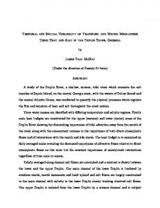
2.3. Methods We used Conditional Sequentia l Gaussian Simulation (CSGS), a stochastic simulation method, to generate realizations of soil biogeochemical properties to describe their spatial patterns and the range of possible outcomes. Conditional Sequential Gaussian Simulation generates conditional cumulative distribution functions (ccdf) for each pixel which captures the uncertainty of predictions. One hundred realizations at a pixel resolution of 100 meters were generated using CSGS. We used a technique suggested by Journel (1983) to construct expected-value estimate maps (E-type maps) summarizing the mean, standard deviation, and other statistical parameters for each pixel location. To assess the accuracy of TP realizations we randomly subdivided the dataset into model (67% of observations) and an independent validation dataset (33% of observations) resulting in 183 model observations and 84 validation observations. The root mean square error (RMSE) was used to evaluate realizations. We used Principal Component Analysis (PCA) to transform a number of possibly correlated biogeochemical variables into a smaller number of uncorrelated variables called principal components (PC) reducing attribute space. The first PC accounts for as much of the variability in the data as possible, and each succeeding component accounts for as much of the remaining variability as possible. Principal components are obtained by projecting the multivariate datavectors on the space spanned by the eigenvectors (Goovaerts, 1997; Wackernagel, 2003). The goal was to identify the significance of biogeochemical properties to explain the variability in the dataset. As a last step CSGS was used to generate realizations of PCs. The emerging spatial patterns of PCs were subdivided into short-, intermediate, and long-range components. Using a step-wise random selection process we reduced the number of observations to 183, 150, 125, 100, 75 and 50 observations respectively for model development and 84 observations for validation. For each data subset we performed the analyses outlined above. The goal was to identify the minimum number of observations required to reproduce the spatial and parameter variability identified using the exhaustive dataset. The results have value to guide future sampling designs in wetlands which are difficult to sample. 3. Results Realization maps were generated for all measured biogeochemical properties. Total phosphorus (TP) is a key variable of interest typically mapped in biogeochemical studies and generated realizations are shown in Figure 1. Specific patterns such as lower TP values in the northern part and higher values in the southern part of the study area prevail on all maps. A crescent shape area in the northern part showed TP as low as 340 mg kg-1 which resemble s natural TP conditions. The cause for high TP values can be attributed to previous P input into the wetland from adjacent agricultural used land. The nutrient enriched soils in the southern part might have been boosted the expansion of Salix caroliniana vegetation which prefers wet mesic soils. The smallest and largest realizations can be interpreted as “best” or “worse” case scenarios of TP predictions rendering the uncertainty of TP predictions. The standard deviation for TP was Null at the observation sites, smallest in the crescent shaped area of low TP predictions, and highest in the southern part of the study area. This suggests that high TP predictions are more uncertain compared to low TP predictions. Total phosphorus observations showed a mean of 619, standard error of mean (SE) of 7.88, median of 601, standard deviation (std.dev.) of 129, minimum of 350, and maximum of 1,014 mg kg-1 . Total phosphorus realizations closely resembled those statistical parameters with a mean of 632, SE of 1.51, median of 624, std.dev. of 107, minimum of 353, and maximum of 1,014 mg kg-1 . Validation analysis of TP resulted in a RMSE of 96 mg kg-1 . Overall, correlations coefficients were low for most variables. However, almost all biogeochemical properties were correlated with each other. The highest significant correlation of 0.805 was between TLON and TLOC. Most correlations were lower; e.g. TP showed significant correlations with BG (0.468), BicTP (0.417), and APA (-0.385). To transform the correlated biogeochemical variables into a smaller number of uncorrelated variables we performed a PCA (Figure 2). The eigenvalues described the amount of the total variance associated with each factor. The first PC contributed 33.91 %, the second PC 15.93 %, and the third PC 11.32 % to the total variance in the dataset. The first three PC accounted for 61.16% of the overall variation in the dataset. The first three principal components accounted for most of the variance and displayed possible interrelations between variables. The circle of correlations in Figure 2 shows the proximity of the variables inside a unit circle and is useful to evaluate affinities and the antagonisms between the variables. The dynamic soil properties TLON (0.3444), TLOC
(0.3309), and BicTP (0.3253) mainly contributed to PC1 and the variables TP (0.3891), TN (-0.3876), and APA (0.3658) mainly contributed to PC2. The third PC was dominated by the contribution of TC (0.6011) and Ash (0.5589).
Smallest realization Realizations of TP in mg kg-1 340 - 400 400 – 460 460 – 520 520 – 580 580 – 640 640 – 700 700 – 760 820 – 880
Mean (100 realizations)
880 – 940 > 940
0
N
4,000
8,000 m
Largest realization
Figure 1. Smallest, mean and largest realizations generated from 267 TP observations using CGSS.
2 (15.93%) F2
r
r
1
3 (11.32%) F3
1 TC
CN
PO
TP BG PI
0.5 PEP
Ash
0.5 CN
Moist CTC
CTC Moist
BicTP
1 F1(33.91%)
TC
0
NH4N
BD
PEP
APA TN
0
TLOC MBP NH4N
TLON MBP TLOC
F2 2 (15.93%) BicTP
TLON BD
-0.5
BG PO PI TP
-0.5 APA
TN Ash
r
-1 -1
-0.5
0
0.5
1
r
-1 -1
-0.5
0
0.5
1
Figure 2. Circle of correlations derived from PCA. The percentage of variance explained by each component is given in parentheses. We created semivariograms of the PCs to analyze their spatial variability (Fig ure 3). The semivariograms were distinctly different with a relatively short range of 1,228 for PC1, a long range of 6,393 for PC2, and an intermediate range of 4,498 m for PC3. These findings indicate that the dataset includes three different sets of spatial autocorrelation representing variability at short, intermediate, and long distances. Labile soil properties
such as TLON, BicTP and TLON showed short-range whereas variables grouped into PC2 such as TP and TN showed a long-range. 0. 1000.2000.3000.4000.5000.6000.7000. 1.25
0.
0. 1000.2000.3000.4000.5000.6000.7000.
1000.2000.3000. 4000.5000.6000.7000.
1.25
M1
1.00
Second PC
3. 1.5
1.001.5
Third PC
3.
0.75 1.0
0.50
0.50
0.25
0.5 0.25
Variance
D1
0.75
Variance
Variance
M1 D1 1.02.
2.
D1 M1
0.51.
1.
First PC 0.00
0. 1000.2000.3000.4000.5000.6000.7000.
0.000.0
0.
Distance (m)
1000.2000.3000. 4000.5000.6000.7000.
0.00.
0. 1000.2000.3000.4000.5000.6000.7000.
Distance (m)
Model: 2 basic structures S1 – Exponential; range: 1,228; sill: 0.984 S2 – Nugget effect; sill: 0.0485
Model: 2 basic structures S1 – Spherical; range: 6,393; sill: 1.152 S2 – Nugget effect; sill: 0.2492
0.
Distance (m)
Model: 2 basic structures S1 – Spherical; range: 4,498; sill: 0.545 S2 – Nugget effect; sill: 0.5945
Figure 3. Semivariograms of the first 3 PCs.
PC1
PC2
PC3
Eigenvalues < -2.5 -2.5 - - 2.0 -2.0 - - 1.5 -1.5 - - 1.0 -1.0 - - 0.5 -0.5 – 0 0 – 0.5 0.5 – 1.0 1.0 – 1.5 1.5 – 2.0 2.0 – 2.5 > 2.5
N
0
4,000
8,000 m
Figure 4. Smallest (top), mean (center) and largest (bottom) realizations of the first three PCs. The semivariograms of PCs reveal different spatial structures with contrasting ranges, nugget, and sill variances (Figure 3). We used CSGS to generate 100 realizations of each PC (Figure 4). Each of the PCs showed distinct spatial patterns with highest eigenvalues in the east-west direction for PC1 and highest eigenvalues in the northsouth direction for PC3. Spatial patterns of PC2 matched closely the spatial patterns generated for TP (compare Figure 1). One important aspect of combining CSGS with PC analysis is to reduce character space focusing on
spatial variability, patterns, and uncertainty of uncorrelated principal components rather than correlated biogeochemical soil properties. The spatial sensitivity analysis using subsets drawn randomly from the exhaustive dataset suggested that dynamic biogeochemical properties grouped into PC1 require sampling densities of > 3.75 sites/100 ha whereas properties grouped into PC2 require a sample density of > 2.52 sites/100 ha to reproduce the spatial patterns and variability across the wetland. 4. Conclusions Our results have implications for future biogeochemical spatial studies. Though more testing of spatial biogeochemical patterns in wetlands are needed our study provides some guidelines to make future sampling in subtropical wetlands in Florida more efficient. Our study focused on decorrelation and attribute variability that facilitate to identify ecological indicators. Future studies can focus on those indicators without mapping the whole suite of biogeochemical properties which is labor intensive and costly. Numerous biogeochemical propertie s showed the same spatial structure across the wetland (e.g. TLOC and TNON) suggesting that processes that generate those properties operate at the same/similar spatial scale. More research is needed to quantify spatial interrelationships and the variability of biogeochemical properties in wetlands.
ACKNOWLEDGEMENTS This study was supported in part by a grant (R-827641-01) from the U.S. Environmental Protection Agency. We thank Yu Wang for the chemical analysis of soil samples. REFERENCES Chilès, J.-P. and P. Delfiner. 1999. Geostatistics – modeling spatial uncertainty. John Wiley & Sons, New York. Craft, C.B. and C. Chiang. 2002. Forms and amounts of soil nitrogen and phosphorus across a longleaf pinedepressional wetland landscape. SSSA J. 66(5): 1713-1721. Deutsch, C. and A. Journel. 1998. GSLIB: Geostatistical software library and user’s guide. Oxford University Press, Oxford, UK. Fisher, M.M. and K.R. Reddy. 2001. Phosphorus flux from wetland soils affected by long-term nutrient loading. J. of Environmental Quality, 30(1): 261-271. Goovaerts, P. 1997. Geostatistics for natural resources evaluation. Oxford University Press, New York. Heuvelink, G.B.M. 1998. Error propagation in environmental modeling with GIS. Taylor & Francis, London. Journel, A.G. 1983. Non-parametric estimation of spatial distributions. Math. Geol. 15: 445-468. Karathanasis, A.D., Y.L. Thompson and C.D. Barton. 2003. Long-term evaluations of seasonally saturated wetlands in western Kentucky. Soils Sci. Soc. Am J. 67(2): 662-673. Lantuéjoul, C. 2002. Geostatistical simulation – models and algorithms. Springer, New York. Reddy, K.R., Y. Wang, W.F. DeBusk, M.M. Fisher, and S. Newman. 1998. Forms of soil phosphorus in selected hydrologic units of Florida Everglades ecosystems. Soil Sci. Soc. Am J. 62(4): 1134-1147. Srivastava, M.R., 1996. An overview of stochastic simulation, pp. 13-22 In Mowrer H.T., Czaplewski R.L., and Hamre R.H. (eds.) Spatial accuracy assessment in natural resources and environmental sciences: Second Int. Symposium. U.S. Dept. of Agriculture, Forest Service, Fort Collins, General Technical Report RMGTR-277. Wackernagel, H. 2003. Multivariate geostatistics – an introduction with applications. Springer, Berlin and New York. White, J.R. and K.R. Reddy. 2000. Influence of phosphorus loading on organic nitrogen mineralization of Everglades soils. Soil Sci. Soc. Am. J. 64(4): 1525-1534.