This article studies a new circuit acyclic clustering problem which divides a combinational circuit into groups of sub-circuits, each of which has limited numbers of ...
Circuit Acyclic Clustering with Input/Output Constraints and Applications Rung-Bin Lin, Tsung-Han Lin, and Shin-An Wu Computer Science and Engineering Yuan Ze University Chung-Li, Taiwan
ABSTRACT This article studies a new circuit acyclic clustering problem which divides a combinational circuit into groups of sub-circuits, each of which has limited numbers of inputs and outputs. Several heuristics are proposed to solving this problem. We achieve 300% speedup on logic simulation, with an application of our approach, for finding an input vector that incurs minimum or maximum leakage power dissipation.
INTRODUCTION
of another gate. We assume that a gate has only an output. A primary input is modeled as a vertex whereas a primary output together with the logic gate driving it is modeled as a vertex. If a circuit is a sequential one, the inputs to flip-flops/latches are treated as primary outputs and the outputs of flip-flops/latches are treated as primary inputs. Our CAC problem is presented below. Given a directed acyclic graph G = (V , E ) where V is a set of nodes and E is a set of directed edges, find a number of groups P1 , P2 ,! , Pd such that (a). Pi is a non-empty subset of V, *∀iPi = V , and Pi � Pj = φ , ∀i ≠ j . (b). FIL ( Pi ) ≤ Bin
Circuit clustering plays an important role for creating a hierarchical design that enables complexity reduction for many design tasks such as verification, physical design, simulation, analysis, etc. It puts together circuit components into groups according to some criteria such as connectivity between components. Circuit components can be logic gates, logic blocks, etc. In this article, we assume that they are logic gates. In addition to minimizing cut size (i.e., the number of nets spanning among different parts; part is similar to group for clustering), circuit clustering may impose some other constraints such as on the number of logic gates in each group and/or the number of groups, etc. If it does so, circuit clustering becomes a vehicle for achieving circuit partitioning [1]. In the past, circuit partitioning (clustering) was mostly done without considering signal flow. Only a few works, most notably those presented in [2] and [3], take signal flow into consideration. When signal flow is considered, it is normally required that no directed cycles should be formed among parts if parts become graph nodes and edges across parts become edges between nodes. We call this kind of problem circuit acyclic partitioning (clustering) problem, CAP (or CAC for clustering) for short. The CAP problem solved in [2] is similar to the conventional graph partitioning problem, which also divides a circuit into a fixed number of parts such that the number of logic gates in a part is within a predefined range. In [3], the authors propose an improved algorithm for such a problem. It is mentioned in [2] that CAP has applications on pipelining in multichip designs, partitioning-based logic minimization, and parallel circuit simulation. Nevertheless, none of these applications were really investigated there. In this article, we presented some heuristics for dealing with a new kind of CAC problem that places a constraint on the number of inputs and outputs in each group rather than on the number of groups and on the size of groups. Our CAC problem is a generalization of decomposing a circuit into k-input lookup tables found in FPGA mapping [4]. It is motivated by trying to speed up logic simulation for finding an input vector that incurs minimum or maximum leakage power dissipation [5-7]. With application of our clustering heuristics, we achieves on average three times speedup on logic simulation for finding minimum/maximum leakage power dissipation. To the best of our knowledge, we were the first to investigate this kind of CAC problem and present a heuristic for it. In the rest of this article, we will present a description of our problem and our CAC algorithms. We will describe how we use clustering results to speed up logic simulation and give some experimental results. Last, we will draw some conclusions.
PROBLEM DESCRIPTION AND RELATED WORK Given us a combinational circuit, we model the circuit as a directed acyclic graph where a vertex represents a logic gate and a directed edge represents a connection from a gate’s output to an input
978-1-4244-2782-6/09/$25.00 ©2009 IEEE
and
FOL( Pi ) ≤ Bout
where
FIL( Pi )
and
FOL ( Pi ) are the set of gates whose outputs are entering and the set of gates whose outputs are going out of group Pi ,
respectively. FIL ( Pi ) and FOL( Pi ) are the numbers of distinct inputs entering and the number of distinct outputs going out of group Pi , respectively. Bin and Bout , two positive integers given by users, place an upper bound on the numbers of inputs and outputs of a group, respectively. (c). The clustered graph is acyclic. A vertex in a clustered graph represents a group and a directed edge in a clustered graph represents a connection from the output of a gate in a group to an input of a gate in another group. A self-loop is not allowed. Our objective is to minimize the total number of groups, i.e., to minimize d. Since our CAC problem allows more than one output in a cluster, it is more complicate than lookup table decomposition for FPGA mapping. It does not impose any constraints on the number of groups and the size of a group. It is therefore quite different from the CAP problem solved in [2] and [3]. A direct extension of using maximum fanout free cone approach like that done in [2,3] is not straightforward. However, our approach still uses the concept of fanout free cone to enforce acyclic property during clustering. Another closely related problem is about packing k-lookup tables into groups for FPGA designs. This packing problem places a constraint on the number of inputs and the number of outputs (i.e., the number of k-lookup table) per group. However, acyclic property is not enforced. Work for this problem is abundant, either for FPGA area or delay minimization [8-13].
HEURISTICS FOR CIRCUIT ACYCLIC CLUSTERING In this section, we first present some terms used in our discourse. The set of fanin nodes of node v, denoted by FI(v), consists of the nodes whose outputs are connected to the inputs of v. A fanin cone of v, denoted by FIC(v), is a subgraph consisting of v and all its predecessors such that any path connecting a node in FIC(v) and v lies in FIC(v) [2]. A k-level fanin cone of v, denoted by FICk(v), is a subgraph of FIC(v) that consists of all the nodes at most k topological levels away from v. The set of fanout nodes of v, denoted by FO(v), consists of the nodes whose inputs are connected to the output of v. A fanout cone of v, denoted by FOC(v) is a subgraph consisting of v and all its successors such that any path connecting a node in FOC(v) and v lies in FOC(v). Let POL denote the set of primary outputs in a circuit under clustering. Our method starts with a group that contains only a few primary outputs whose fanin cones are strongly overlapped. Although the primary inputs are modeled as vertices, they each will be treated as a
110
pseudo cluster and will not be included into any other clusters. The details of our method are presented below and its pseudo code is shown in Fig. 1. Step 1. Initially, we select some highly-related primary outputs (POs) and put them into a cluster C (line 4). To determine which POs are highly related, we first construct a k-level fanin cone for each PO i, denoted by FICk(i). We then use the following formula to determine the closeness of two POs i and j. FICk (i) ∩ FICk ( j ) (1) closeness (i, j ) = min( FICk (i) , FICk ( j ) ) closeness(i,j) = 1 means either FICk (i) ⊆ FICk ( j ) or FICk (i) ⊇ FICk ( j ) . We first select a pair of POs with the highest closeness and put these two POs into C. We then repeatedly add into C a new PO h with the maximum closeness(h, j) for h ∉ C and j ∈ C if FIL (C ) ≤ 0.9Bin and FOL(C ) ≤ Bout still hold after PO h is added into C. Once cluster C is created, a fanin list FIL(C) is also created (line 5). Step 2. We select a node v with the largest gain from FIL(C) (line 7). If we can not find such a node, i.e., FIL(C) is empty, go to Step 5 (line 26). Otherwise, we check whether including v into C will cause a violation of the input and output size bounds (starting from line 8 with Check(v) procedure in Fig. 2). We will give two ways of computing gain later. A node v can be included into C if including all nodes in FOC(v) will not violate the input and output size bounds. The reason for including all nodes in FOC(v) into C is to maintain the acyclic property. Step 3. If including all nodes in FOC(v) into C does not violate the input and output size bounds, we will do so. We then remove v from FIL(C) but add FI(v) into FIL(C) (lines 9~11). Go back to Step 2. Step 4. If v can not be included into C due to the violation of input or output size bounds for the time being, we do not drop v immediately, but check its fanin nodes in FI(v) instead to see whether we can include a node u in FI(v) into C. If there exists such a node, we remove v from FIL(C), but include FOC(u) into C and add FI(u) into FIL(C) (lines 21~23). Go back to Step 2. Otherwise, we remove v from FIL(C) (lines 18~19) if all nodes in FI(v) has been inspected. Go back to Step 2. If not all nodes in FI(v) has been checked, repeat this Lookahead step. Step 5. After forming a new cluster C, we write out C. We then remove the nodes and edges in this cluster from the original circuit (line 27). We treat those nodes whose outputs do not connect to any nodes in the remaining circuit as new primary outputs and add them into POL. We then remove the primary outputs going out of cluster C from POL (line 28). Go back to Step 1 if the remaining circuit G still has logic gates. We limit the number of inputs per cluster not more than 0.9 Bin in order to include some other non-primary output nodes into a cluster later. We find that coefficient 0.9 produces the best results for the benchmark circuits investigated in this work. Informally, we can show that our approach create only an acyclic clustered circuit. Given the example in Fig. 3, if there is a cycle in a clustered circuit, two scenarios are possible. The first scenario shown in Fig. 3(a) is a self-loop. However, this is not possible because the edge feedback into the cluster should completely fall inside the cluster. The second scenario is shown in Fig. 3(b). This is also not possible. Suppose gates 4 and 5 must be in the same cluster. Based on our approach, gate 1 must be in the same cluster as gates 4 and 5. Hence, no cycle is possible. Conversely, if gates 4 and 5 are in two different clusters, gate 1 must be in another cluster or in the cluster where gate 5 resides. Hence, no cycle exists among these clusters. Fig. 4 illustrates an example of the above clustering process with input and output size bound set equal to 5. In the beginning, we have POL={1,2,3}. In Fig. 4(a), the input cone for gates 1, 2, and 3 are {1,5,6,7,8,9,10,11}, {2,4,5,6,7,8,9,10, 11}, and {3,11}, respectively. We first put PO gate 1 and PO gate 2 into cluster C because they are most strongly related. We later add PO gate 3 into C as shown in Fig. 4(b). Now we have C={1,2,3} and FIL(C)={4,5,11}. We subsequently include gates 4 and 5 into C. At this moment, we have C={1,2,3,4,5} and FIL(C)={6,11}. We then try to include gate 6 into C, but it is found to be violating input size bound as shown in Fig.
Algorithm: Circuit_Acyclic_Clustering(G) Input: A directed acyclic graph G representing a circuit design Output: A set of clusters each consisting of a set of logic gates 1. POL= all the primary outputs of G; 2. Do 3. cluster C = ∅ ; 4. PO_selection(C,POL); // Return C, a set of primary outputs treated as seeds for clustering 5. Create FIL(C); 6. Do 7. Select a node v with the largest gain from FIL(C); 8. If (Check(v)) { 9. Remove v from FIL(C); 10. Include FOC(v) into C; 11. Push FI(v) into FIL(C); } 12. Else { // lookahead 13. Fanin_list LA = FI(v); 14. While (LA is not empty) { 15. Select a node u from LA; If (!Check(u)) { 16. 17. Remove u from LA; 18. If (LA is empty) // dropping v 19. Remove v from FIL(C); } 20. Else { // including u into C 21. Include FOC(u) into C; 22. Remove v from FIL(C); 23. Push FI(u) into FIL(C); 24. break; } // end Else } // end while } // end Else 25. Until FIL(C) is empty; 26. Output(C); // Write out a cluster C 27. All nodes and edges in C and edges input to or output from C are removed from G; 28. Update POL; // creating new POs after forming a cluster 29. Until G is empty;
Fig. 1. Circuit acyclic clustering algorithm.
Algorithm: Check (v) Input: a node v in G Output: Flagging whether node v should be included into C 1. If (including FOC(v) into cluster C will not make C violate the input/output size bounds) 2. return true; 3. Else 4. return false;
Fig. 2. Acyclic constraint check. 4(c). Now, we perform the lookahead procedure in Step 4. We currently have LA={7,8}. We find that gates 7 and 6 can be included into C as shown in Fig. 4(d). Now, we have C={1,2,3,4,5,6,7} and FIL(C)={8,11}. We continue to include gate 10 (by lookahead), gate 8, and gate 9 into C. A new cluster C={1,2,3,4,5,6,7,8,9,10} is thus created as shown in Fig. 4(e). At this moment, we write out C and then remove it from the circuit graph. The program execution goes back to line 1. So we have POL={11}. A new cluster grows just like the one we had it before. Finally, we have clusters for the whole circuit shown in Fig. 4(f). Note that we do not use gain functions here. Since there can be more than one candidate in FIL(C) for being included into C, we can either randomly include one of them or using some criteria to select a candidate. To form a larger cluster, we would like to include a gate so that more gates can be brought into C but as fewer inputs as possible are added to C. Hence, we introduce the following gain function for g ∈ FIL(C ) .
111
Fig. 3. Proof of acyclic.
fewer large-sized super gates can be used to speed up logic simulation. In our work, for each cluster with i inputs and j outputs, we create a 2i by (j+1) table. The first j columns are used to store the output logic values for j outputs, respectively. The last column is used to store leakage power data for all input vectors. Then, each cluster will be modeled as a super gate accompanied with a 2i by (j+1) table and logic simulation just goes on as usual. Basically, each table is unique and must be created prior to logic simulation. To curtail table size, i is generally not more than 20.
EXPERIMENTAL RESULTS Acyclic Clustering
Fig. 4. An example of clustering. # of gates brought into C + forwardGain( g ) (2) # of inputs increased The forwardGain of g is defined as follows: FO( fi ) forwardGain( g ) = Max( (3) ), ∀fi ∈ FI ( g ) FI ( fi ) A larger forwardGain implies that, after including g into C, the gates pushed into FIL(C) will have larger fanout with respect to the numbers of their fanins. For example, forwardGain(5)=1/2 for gate 5 in Fig. 4(b) whereas forwardGain(6)=2/2 for gate 6 in Fig. 4(c). The second gain function for node g ∈ FIL(C ) is as follows. gain( g ) =
gain( g ) =
Level _ Diff ( g , h) × FO( g )
+ forwardGain( g ) (4) FI ( g ) Level_Diff(g,h) is the minimum difference between the topological level of a node h ∈ FO( g ) in C and that of node g. The product of Level_Diff(g, h) and FO( g ) approximates the number of gates that might be brought into C if g is included into C. We actually give a higher preference for a node g ∈ FIL(C ) that has a smaller level number. Note that the level number of h is greater than the level number of g. A primary input has a level number of zero. The time complexity of the proposed approach is somewhat hard to analyze accurately. Roughly, the worst-case time complexity of our algorithm is O (dn 2 ) where d is the number of clusters and n is the number of gates. Hence, if input and output size bound is larger, we will have a smaller d and thus spend less time for clustering.
We have implemented four variants of our clustering approach. One is without lookahead and without using gain function (NL), one is with lookahead but without using gain function (LH), one is with lookhead and using the gain function in (2) (LG1), and one is with lookahead and using the gain function in (4) (LG2). For the purpose of comparison, we also implemented a VPack like algorithm (VP) [9]. VPack is a synthesis tool for FPGA with input/output and capacity constraints. Because our problem does not have capacity constraint, our implementation of VP only does a lookahead step during its hill-climbing phase as we did for LH. This VPack-like approach practically gives us lower bounds on the number of clusters that can be achieved by our approaches because it allows a cycle in a clustered graph. Some ISCAS and ITC’99 benchmark circuits are employed for our experiments. The circuits are synthesized using a 0.18um commercial cell library. The number of levels for backward tracing from primary outputs to find out closely related primary outputs is set to five in our experiments for the best results. The input size bound and output size bound are equal and set to 10, 12, 14, 16, 18, and 20. Due to limited space, Table 1 shows only the clustering results for size bound of 14. Table 2 shows the average number of clusters. The numbers there are obtained as follows. For each circuit, we first compute a normalized number of clusters with respect to that obtained by LH for each input and output size bound. The normalized numbers of clusters for each circuit with different input and output size bounds are averaged to give a number shown in Table 2. As one can see, the results obtained by our methods are not much different. LH is on average the best. However, VP has 22% fewer clusters than LH. In Table 2, we also show input saturation degree which is the ratio of the number of inputs to a cluster to the input size bound. Output saturation degree can be defined similarly. Output saturation degrees are normally ranged from 40% to 60% (not shown here) whereas input saturation degrees are all larger than 90%. This shows that cluster growth is limited by the input size bounds rather than output size bounds. The drawback of our heuristics is lack of a global view on the problem. Therefore, heuristics capable of using global characteristics of a circuit are yet to be developed to achieve better results. The time for clustering using LH in general decreases with increasing input and output size bounds as shown in Table 3. This corresponds quite well to the time complexity analysis made in the previous section. However, clustering time does not vary much across different approaches for given input and output size bounds because all the approaches differ only in the way of lookahead. Note that the data in Table 3 are obtained from the clustering experiments done in the next subsection where circuits are synthesized using a simpler cell library.
APPLICATION ON LOGIC SIMULATION In this section we describe how to employ the clustering results for speeding up leakage power computation using logic simulation. Although logic simulation is not the best way of doing such task, it is simplest and usually taken as a base methodology for comparison. ˟ogic simulation is generally slow, but circuit clustering that transforms a circuit of many small-sized gates into a circuit with
112
Table 1. Number of clusters obtained using different approaches. c6288 c7552 s35932 s38417 s38584 b14 b15 b20 b21 b22 SUM
# of gates 1227 733 2783 2782 4800 2227 2927 5006 4730 7768
LH 86 67 329 339 488 274 474 611 565 940 4173
NL 84 69 329 343 495 276 475 614 568 954 4207
LG1 88 73 343 350 523 286 458 638 577 979 4315
LG2 83 65 327 339 493 279 479 611 569 934 4179
VP 77 41 294 280 434 196 344 449 419 690 3224
Table 2. Normalized number of clusters with respect to LH versus input saturation degrees. c6288 c7552 s35932 s38417 s38584 b14 b15 b20 b21 b22 Ave
LH 1 1 1 1 1 1 1 1 1 1 1
Normalized # of clusters NL LG1 LG2 VP 0.995 1.033 0.978 0.888 0.996 1.079 1.006 0.630 1.000 1.027 0.986 0.880 1.018 1.027 1.012 0.821 1.019 1.079 1.014 0.902 1.013 1.049 0.999 0.728 1.008 0.979 1.007 0.734 1.007 1.047 1.004 0.730 1.007 1.037 1.009 0.735 1.013 1.042 1.003 0.735 1.008 1.040 1.002 0.778
clustering results on logic simulation for finding an input vector that incurs minimum or maximum leakage power dissipation was investigated. On average, a speedup of three times was observed.
Input saturation degree (%) LH NL LG1 LG2 VP 96 96 97 97 99 97 96 99 97 98 96 96 100 98 99 94 94 98 94 99 96 96 99 96 100 96 96 99 96 99 92 92 98 92 99 96 95 99 96 100 96 96 99 96 100 96 95 99 96 100
Table 4. Simulation speedup. # of gates c6288 2332 c7552 1103 s35932 5664 s38417 7163 s38584 8292 b14 4059 b17 22372 b20 9661 b18 55444 b15 7264 b21 8825 b22 14725 Ave
Table 3. Clustering time for different input size bounds (sec). input size s38584 s38417 s35932 b14 bound 8 605 408 894 25 9 555 366 778 19 10 482 309 770 19 11 381 287 550 14 12 354 264 674 13
b15
b17
b18
b20
b21
b22
114 102 85 69 68
2974 2540 2192 1878 1642
34121 31013 27268 25401 21923
138 109 107 81 78
138 112 91 80 79
480 386 325 277 263
ct (s) 0.18 0.16 733 326 475 18 2245 103 26401 88 100 346
st1p (s) stxp (s) st1p/(ct+stxp) st1p/stxp 1109 271 4.09 4.09 1922 340 5.65 5.65 4832 3045 1.28 1.59 7157 3778 1.74 1.89 8857 3053 2.51 2.90 4448 1108 3.95 4.01 45915 22820 1.83 2.01 9615 3134 2.97 3.07 302416 116296 2.12 2.60 10643 3285 3.16 3.24 22208 4151 5.22 5.35 31634 12427 2.48 2.55 3.08 3.25
Applications on Speeding Up Logic Simulation In this subsection, we present some experimental data for an application of our approach to logic simulation. Logic simulation is performed to find out the maximum/minimum leakage power dissipation of a circuit. Since the 0.18um cell library used in the previous subsection does not contain any leakage power data, we build a new library using 45nm technology based on BPTM [14]. The simulation models for transistors are based on BSIM4 [15]. The cell library consists of NANDs, NORs, XORs, inverters and flip-flop with different driving capabilities. Winspice [16] is employed to perform circuit simulation to obtain the leakage power for each input vector of a logic gate. Benchmark circuits are synthesized using Synopsys Design Compiler with our cell library. All experiments in this work are run on Intel Xeon 2.33GHz with 32G bytes memory. Our clustering approach (LH) is used to perform circuit clustering. The input and output size bounds are equal. Their values vary from 8 to 12. To create a lookup table for each distinct cluster (super gate), a logic simulator obtained from [17] is modified to perform logic simulation for finding the leakage powers and output responses for all input vectors to the cluster (super gate). Since the number of inputs to a cluster is not more than 20, the number of entries in a lookup table will be not more than one million. The memory used for simulation is bounded by O (d 2i j ) where d is the number of clusters, i is input size bound, and j is output size bound. The same logic simulator is further modified to simulate a clustered circuit using lookup tables for clusters. Sixteen millions of vectors are simulated for each circuit. Clustering and simulation results are presented in Table 4. The numbers of gates (not counting flip-flops) are much larger than that presented in Table 1. This is due to the use of simpler gates for logic synthesis here. The column denoted by ct gives the average clustering time in seconds with input and output size bounds ranging from 8 to 12. The column st1p gives the time for simulating a circuit without clustering. The column stxp gives the average time for simulating a clustered circuit with input and output size bounds ranging from 8 to 12. The column st1p/stxp gives the simulation speedup without counting clustering time whereas the column st1p/(ct+stxp) gives the simulation speedup with counting clustering time. On average, we achieve 3 times speedup. Fig. 5 shows how speedup varies with input size bound. In addition to the applications presented here, applications of our approach to other area such as physical design are possible.
CONCLUSIONS
Fig. 5. Speedup versus input size bound.
REFERENCES [1] [2] [3] [4] [5] [6] [7] [8] [9] [10] [11] [12] [13]
[14] [15]
In this article we studied a new circuit acyclic clustering problem. Four heuristics with varying rules of selecting candidates for growing clusters were investigated. LH that uses a simple rule with hill climbing lookahead obtained the best results. An application of
113
[16]
[17]
C. Fiduccia and R. Mattheyses, ‘‘A linear time heuristic for improving network partitions,’’ Design Automation Conf., pp. 175-181, 1982. J. Cong, Z. Li, and R. Bagrodia, “Acyclic multi-way partitioning of boolean networks,” Design Automation Conference, pp. 670–675, 1994. E. S. H. Wong, E. F. Y. Young, and W. K. Mak, “Clustering based acyclic multi-way partitioning,” Great Lakes Symposium on VLSI, pp.203-206, 2003. J. Cong and Y. Ding, “FlowMap: An optimal technology mapping algorithm for delay optimization in Lookup-Table Based FPGA Designs,” IEEE Trans. On CAD, pp. 1-12, Jan. 1994. J. P. Halter and F. N. Najm, “A gate-level leakage power reduction method for ultra-low-power CMOS circuits,” Custom Integrated Circuits Conference, pp. 475-478, 1997. G. W. Liao, J. S. Feng, and R. B. Lin, “A divide-and- conquer approach to estimating minimum/maximum leakage current,” ISCAS Vol. 5, pp. 47174720, 2005. Z. Chen, M. Johnson, L. Wei, and K. Roy, “Estimation of standby leakage power in CMOS circuits considering accurate modeling of transistor stacks,” ISLPED, pp. 239-243, 1998. V. Betz and J. Rose, “Cluster-based logic blocks for FPGAs: area-efficiency vs. input sharing and size,” Custom Integrated Circuits Conference, pp. 551554, 1997 V. Betz and J. Rose, “VPR: A new packing, placement and routing tool for FPGA Research,” International Workshop on Field Programmable Logic and Applications, pp. 213-222, 1997. E. Ahmed and J. Rose, “The effect of LUT and cluster size on deep-submicron FPGA performance and density,” IEEE Trans. On VLSI Systems, Vol. 12, No. 3, pp. 288-298, March 2004. A. Marquart, V. Betz, and J. Rose, “Using cluster-based logic blocks and timing-driven packing to improve FPGA speed and density,” International ACM Symposium on Field-Programmable Gate Arrays, pp. 37-46, 1999. Z. Marrakchi, H. Mrabet, H. Mehrez, “Hierarchical FPGA clustering based on multilevel partitioning approach to improve routability and reduce power dissipation,” International Conference on Reconfigurable Computing, 2005. A. Singh, G. Parthasarathy, M. Marek-Sadowska, “Efficient circuit clustering for area and power reduction in FPGAs,” ACM Transactions on Design Automation of Electronic Systems (TODAES), Vol. 7, No. 4, pp. 643-663, 2002. http://www.eas.asu.edu/~ptm/ X. Xi, M. Dunga, J. He, W. Liu, K. M. Cao, X. Jin, J. J. Ou, M. Chan, A. M. Niknejad, and C. Hu, BSIM4.3.0 MOSFET Model- User’s Manual, 2003. http://www.ousetech.co.uk/winspice2/ Lee, H. K. and D. S. Ha, “An efficient, forward fault simulation algorithm based on the parallel pattern single fault propagation,” Design Automation Conference, 1992, pp. 291-299.