As an illustration, Figure 1 shows a two dimensional input space with two classes (pos- itive + and negative â). The distribution of examples pre- cludes a simple ...
Class Decomposition Via Clustering: A New Framework For Low-Variance Classifiers Ricardo Vilalta, Murali-Krishna Achari, and Christoph F. Eick Department of Computer Science University of Houston Houston TX, 77204-3010, USA {vilalta, amkchari, ceick}@cs.uh.edu
Abstract In this paper we propose a pre-processing step to classification that applies a clustering algorithm to the training set to discover local patterns in the attribute or input space. We demonstrate how this knowledge can be exploited to enhance the predictive accuracy of simple classifiers. Our focus is mainly on classifiers characterized by high bias but low variance (e.g., linear classifiers); these classifiers experience difficulty in delineating class boundaries over the input space when a class distributes in complex ways. Decomposing classes into clusters makes the new class distribution easier to approximate and provides a viable way to reduce bias while limiting the growth in variance. Experimental results on real-world domains show an advantage in predictive accuracy when clustering is used as a preprocessing step to classification.
1
INTRODUCTION
Classification and clustering stand as central techniques in data analysis. Classification aims at deriving a prediction model from labelled data. The model is intended to capture correlations between the feature variables and the target variable to predict the class label of new data objects. Clustering is a useful tool in revealing patterns in unlabelled data; the goal is to discover how data objects gather into natural groups. The work described in this paper explores how classification algorithms can benefit from class density information that is obtained using clustering. These information can be exploited to improve the quality of the decision boundaries during classification and enhance the prediction accuracy of simple classifiers. We demonstrate how using classification and clustering techniques in conjunction addresses key issues in learning theory (e.g., locality vs capacity or bias vs variance) and provides an attractive new
family of classification models. Our goal is to exploit the information derived from a clustering algorithm to increase the complexity of simple classifiers characterized by low variance and high bias. These algorithms, commonly referred to as model-based or parametric-based, encompass a small class of approximating functions and exhibit limited flexibility in their decision boundaries. Examples include linear classifiers, probabilistic classifiers based on the attribute-independence assumption (e.g., Naive Bayes), and single logical rules. The question we address is how to increase the complexity of these classifiers to tradeoff bias for variance in an effective manner. Since these models start off with simple representations, increasing their complexity is expected to improve their generalization performance while still retaining their ability to output models amenable to interpretation. Our approach consists of increasing the degree of complexity of the decision boundaries of a simple classifier by augmenting the number of boundaries per class. The idea is to transform the classification problem by decomposing each class into clusters. By relabelling the examples covered by each cluster with a new class label, the simple classifier generates an increased number of boundaries per class, and is then armed to cope with complex distributions where classes cover different regions of the input space. Not every cluster is relabelled with a new class; our algorithm explores the space of possible new class assignments in a greedy manner maximizing predictive accuracy. In summary our approach comprises the following modules: 1. A pre-processing step to classification that consists of clustering examples that belong to the same class. This identifies regions of high class density. 2. A search for a configuration of class assignments over the set of clusters that optimizes predictive accuracy. This increases the number of decision boundaries per class.
3. A function that maps the predicted class label of a test example to one of the original classes. This transforms the auxiliary set of new classes into the original set of classes. We test our methodology on twenty datasets from the University of California at Irvine repository, using two simple classifiers: Naive Bayes and a Support Vector Machine with a polynomial kernel of degree one. Results denote a significant increase in predictive accuracy when our classdecomposition approach is applied (Section 6). To conclude, empirical results support our goal statement that preidentifying local patterns in the data through clustering is a helpful tool in improving the performance of simple classifiers. The paper organization is described next. Section 2 introduces background information and our problem statement. Section 3 details our class decomposition approach via clustering to improve the performance of simple classifiers. Section 4 uses the VC dimension to understand the increase in representational power gained with our approach. Section 5 reviews related work. Section 6 reports an empirical assessment of our approach. Finally, Section 7 states our summary and future work.
2 2.1
PROBLEM STATEMENT SIMPLE DISCRIMINANT FUNCTIONS
Let (X1 , X2 , · · · , Xn ) be an n-component vector-valued random variable, where each Xi represents an attribute or feature; the space of all possible attribute vectors is called the attribute or input space X . Let {y1 , y2 , · · · , yk } be the possible classes, categories, or states of nature; the space of all possible classes is called the output space Y. A classifier receives as input a set of training examples T = {(x, y)}, where x = (x1 , x2 , · · · , xn ) is a vector or point in the input space (xi is the value of attribute Xi ) and y is a point in the output space. The outcome of the classifier is a function h (or hypothesis) mapping the input space to the output space, h : X → Y. We consider the case where a classifier defines a discriminant function for each class gj (x), j = 1, 2, · · · , k and chooses the class corresponding to the discriminant function with highest value (ties are broken arbitrarily): h(x) = ym iff gm (x) ≥ gj (x)
(1)
Possibly, the simplest case is that of a linear discriminant function, where the approximation is based on a linear model: gj (x) = w0 +
n X i=1
wi x i
(2)
where each wi , 0 ≤ i ≤ n, is a coefficient that must be learned by the classification algorithm. We will also consider probabilistic classifiers where the discriminant functions are proportional to the posterior probabilities of a class given the input vector x, P (yj |x). The classifier, also known as Naive Bayes, assumes feature independence given the class [7]: gj (x) = P (yj )Πni P (xi |yj )
(3)
where P (yj ) is the a priori probability of class yj , and Πni P (xi |yj ) is a simple product approximation of P (x|yj ), called the likelihood or class-conditional probability.
2.2
THE BIAS-VARIANCE TRADEOFF
Simple discriminant functions tend to output poor function approximations when the data distributes in complex ways. Our goal is to increase the complexity of simple classifiers to obtain better function approximations. Since our training set comprises a limited number of examples and we do not know the form of the true target distribution, our goal is inevitably subject to the bias-variance dilemma in statistical inference [9, 10]. The dilemma is based on the fact that prediction error can be decomposed into a bias and a variance component1 ; ideally we would like to have classifiers with low bias and low variance but these components are inversely related. On the one hand, simple classifiers, commonly referred to as model-based or parametric-based –and the subject of our study–, encompass a small class of approximating functions and exhibit limited flexibility on their decision boundaries. Their small repertoire of functions produces high bias (since the best approximating function may lie far from the target function) but low variance (since there is little dependence on local irregularities in the data). Examples include linear classifiers, probabilistic classifiers such as Naive Bayes, and single logical rules. On the other hand, increasing the complexity of the classifier reduces the bias but increases the variance. Complex classifiers, also referred to as model free or parametric-free, encompass a large class of approximating functions; they exhibit flexible decision boundaries (low bias) but are sensitive to small variations in the data (high variance). Examples include neural networks with a large number of hidden units and k-nearest neighbor classifiers with small values for k. Our problem statement can be rephrased as follows: how can we decrease the bias (i.e., increase the complexity) of our simple classifiers without drastically increasing the variance component? Notice our goal sets forth in a direction 1 A third component, the irreducible error or Bayes error, cannot be eliminated or tradeoff.
X2
X2
(a)
X1
(b)
X1
Figure 1. (a) A high-order polynomial improves the classification of a linear classifier at the expense of increased variance. (b) Increasing the number of linear discriminants guided by local patterns increases complexity with lower impact on variance. Algorithm 1: Mapping-Process Input: clustering method C, dataset T orthogonal to combination methods like bagging [5] and Output: new dataset T 0 boosting [8] where the goal is to reduce the variance comM APPING -P ROCESS(C,T ) ponent in generalization error by voting on variants of the (1) Separate T into subsets {Tj } training data. (2) where Tj = {(x, y) ∈ T |y = yj } (3) foreach Tj 2.3 INCREASING COMPLEXITY THROUGH (4) Apply clustering C on Tj ADDITIONAL BOUNDARIES (5) Let {Cpj } be the set of clusters (6) foreach example e = (x, yj ) (7) Let p be the cluster index for x Our solution is to exploit information about the distribu(8) Create example e0 = (x, yj0 ) tion of examples through a pre-processing step that iden(9) where yj0 = (yj , p) tifies natural clusters in data. As an illustration, Figure 1 (10) Add e0 to T 0 shows a two dimensional input space with two classes (pos(11) end itive + and negative −). The distribution of examples pre(12) end cludes a simple linear classifier attaining good performance (13) return T 0 (Figure 1a, bold line). One way to increase the complexity of the classifier is to enlarge the original space of linear Figure 2. The process to transform dataset combinations to allow for more flexibility on the decision T into a new dataset T 0 using a clustering boundaries, for example by adding higher order polynomialgorithm. als (Figure 1a, dashed line). But this comes at the expense of increased variance and possibly data overfitting. 3.1 CLASS DECOMPOSITION Alternatively, one can retain the same space of linear functions but increase the number of decision boundaries The first module pre-processes the training data by clusper class (Figure 1b). This increases the complexity of the tering examples that belong to the same class as shown in classifier but with less impact on variance (Section 4). The Algorithm 1 (Figure 2). We proceed by first separating trick lies on identifying regions of high class density within dataset T into sets of examples of the same class. That is subsets of examples of the same class which we accomplish T is separated into different sets of examples T = {Tj }, through clustering. The next sections provide a detail dewhere each Tj comprises all examples in T labelled with scription of our approach. class yj , Tj = {(x, y) ∈ T |y = yj }. For each set Tj we apply a clustering algorithm C to find 3 CLASS DECOMPOSITION VIA CLUSsets of examples (i.e., clusters) grouped together according TERING to some distance metric over the input space2 . Let {cji } be the set of such clusters. We map the set of examples in 0 T j into a new set Tj by renaming every class label to inOur solution comprises three modules: 1) a decomposidicate not only the class but also the cluster to which each tion of classes into clusters; 2) a search for an optimal class example belongs. One simple way to do this is by makassignment configuration; and 3) a function mapping predictions to the original set of class labels. We explain each module in turn.
2 We consider a flat type of clustering (as opposed to hierarchical) where each object is assigned to exactly only cluster.
X2
X2
{(x,y’)| y’ = (+,2)}
{(x,y’)| y’ = (-,1)} {(x,y’)| y’ = (+,1)}
X1
X1
Figure 3. The mapping process relabels examples to encode both class and cluster.
Figure 4. An example where merging clusters can further increase accuracy performance.
ing each class label a pair (a, b), where the first element represents the original class and the second element represents the cluster that the example falls into. In that case, Tj0 = {(x, yj0 )}, where yj0 = (yj , i) whenever example x is assigned to cluster cji . An illustration of the transformation above is shown in Figure 3. We assume a two-dimensional input space where examples belong to either class positive (+) or negative (−). Let’s suppose the clustering algorithm separates class positive into two clusters, while class negative is grouped into one single cluster. The transformation relabels every example to encode class and cluster label. As a result, dataset T 0 has now three different classes. Finally the new dataset T 0 is simply the union of all sets of examples of the same class relabelled according to the cluster to which each example Sk belongs, T 0 = j=1 Tj0 . In summary, the first module maps training set T into another dataset T 0 through a class-decomposition process. The mapping leaves the input space X intact but changes the output space Y into a (possibly) larger space Y 0 (i.e., |Y 0 | ≥ |Y|, where | · | is the cardinality of the space).
to merge clusters derived from the first step. Following the same notation as before, a class label will be a pair (a, b), where the first element represents the original class label and the second element represents the cluster that the example falls into; but the difference now is that two or more clusters may correspond to the same second element (i.e., element b), which can be interpreted as having clusters merged into a single cluster. In Figure 4, for example, the class decomposition process (module 1) produces four new class labels: (+, 1), (+, 2), (+, 3), and (−, 1). If we observe an increase in predictive accuracy by merging the two top positive clusters into one positive cluster, module 2 would recommend a class assignment based on three labels only: (+, 1), (+, 2), (−, 1), which is better suited for a simple classifier. Our goal is to explore the space of possible ways to merge clusters obtained during the first step, until we find a configuration that maximizes predictive accuracy (over a validation set different from the training set). The space of possible configurations corresponds to the space of all subsets of clusters, with each subset being assigned the same cluster index (i.e., being assigned the same class label). Obviously one cannot explore this space exhaustively. If class yj is decomposed into nj clusters, the number of different configurations has an upper bound of O(2nj ). To avoid an exhaustive search we follow a heuristic greedy approach. Figure 5, Algorithm 2, describes our approach. The search starts by evaluating predictive accuracy assuming each cluster is mapped to a separate index. Next we start looking for pairs of clusters (e.g. {cj1 , cj2 }) and compute predictive accuracy assuming the two clusters on each pair are mapped to the same index. We then take those pairs for which predictive accuracy increased and rank them accordingly. To enforce a mutually exclusive list of clusters we prune every cluster pair where one cluster appears on another pair with higher rank. Next we construct 3-element cluster sets by adding single clusters to the remaining 2-element cluster sets found
3.2
A SEARCH FOR THE OPTIMAL CLASS ASSIGNMENT
Increasing the number of classes according to the number of induced clusters does not always yield optimal performance. As an illustration, Figure 4 shows a distribution of examples where the positive class decomposes into three clusters. Constructing a linear classifier separately on each cluster generates decision boundaries that cause misclassifications (top positive clusters in Fig 4, bold lines). One solution is to maintain the lower cluster while reverting part of the decomposition process by merging the top clusters into one cluster. This creates a decision boundary (Fig. 4, dashed line) that allows separating the two classes without errors. Our second module explores the space of possible ways
Algorithm 2: Merge-Clusters-Process Input: initial dataset T 0 Output: modified dataset T 0 M ERGE(T 0 ) (1) foreach class yj (2) Let Cj = {cji } be the set of clusters (3) Let L1 = Cj (4) Let i = 2 be the search level (5) repeat (6) Li ← form subsets of clusters of size i (7) by combining Li−1 with Cj (8) Evaluate and rank all new subsets (9) Prune lower rank subsets with (10) duplicated clusters (11) i←i+1 (12) until no accuracy improvement (13) T 0 ← change T 0 such that examples covered (14) by clusters within the same subset have same (15) class label (16) end (17) return T 0 Figure 5. Improving predictive accuracy by merging clusters of examples on each class.
in the previous step, and evaluate their predictive accuracy (now assuming that all three clusters are mapped to the same index). We keep those for which predictive accuracy increased and apply pruning as we described before. The algorithm terminates when no new cluster sets of higher cardinality can be produced from the cluster sets in the previous iteration. Finally, we prune any lower cardinality cluster sets that have a cluster in common (i.e., that overlap) with a higher cardinality set. At that point we assign the clusters on each subset the same index (i.e., the same class label). As an illustration, assume class y1 decomposes into six different clusters. Initially each cluster forms a unique set and is assigned a different index: {c11 }, {c12 }, · · · , {c16 }. Now assume the following cluster pairs show improvement in predictive accuracy (ranked accordingly): {c12 , c13 }, {c11 , c14 }, {c11 , c15 }. The last cluster pair is eliminated since cluster c11 appears on a higher ranking pair. At the next level assume the following 3-element cluster is obtained: {c12 , c13 , c15 }. If no more cluster sets are produced, then the last step simply prunes lower cardinality cluster sets that have a cluster in common. The final configuration indicates how clusters are merged together. For example, {c12 , c13 , c15 }, {c11 , c14 }, {c16 } indicates clusters two, three, and five are merged into a single cluster, the same holding true for clusters one and four; cluster six is not merged. The final training set divides class y1 into three new categories.
3.3
IMPROVING COMPUTATIONAL EFFICIENCY
Clearly, searching over the space of cluster subsets demands excessive computational power. To ease the burden of estimating predictive accuracy often, we note that changing class assignments over the clusters on a particular class does not affect the discriminant functions corresponding to other classes. Therefore in estimating predictive accuracy one can keep all discriminant functions fixed except for the one corresponding to the class under analysis. This reduces the computational cost of our approach by a factor proportional to the number of classes.
3.4
CLASSIFICATION OF EXAMPLES
Our last module shows how to assess the performance of the linear classifier over the extended output space. This is necessary during the search over the space of subsets of clusters (Section 3.2), and while estimating final predictive accuracy. During learning, the simple classifier is trained over dataset T 0 producing a hypothesis h0 mapping points from input space X to the new output space Y 0 . During classification, hypothesis h0 will output a prediction consisting of a class label and a cluster label, h0 (x) = (a, b). To know the actual prediction in the original output space Y we simply remove the cluster index. Essentially, we predict class label yj whenever example x is assigned to any of the clusters (or subsets of clusters) of class yj . As an illustration, assume the prediction of an example x is h0 (x) = (−, 1), then our final prediction simply disregards the cluster index and assigns x to the negative class. Our class decomposition process aims at eliminating distributions unfavorable to simple classifiers where a class spreads out into multiple regions. As each cluster (or group of clusters) is transformed into a class of its own, each class sits in a tight region and becomes easier to separate away using simple decision boundaries.
4
COMPLEXITY AND THE THE VC DIMENSION
In this section we use a measure of complexity known as the VC dimension to compare the increase in representational power gained by augmenting the number of decision boundaries of a simple classifier (our approach) to the increase gained by augmenting the flexibility of the decision boundaries. Consider that a simple classifier has a small class of functions φ from which to draw a hypothesis. If we wish to make our class φ stronger we must increase the representational power of its member functions. Recall, however, that adding too much representational power
would increase the variance component of classification error (Section 2.2). Here we provide evidence showing that our approach increases the representational power of φ in small steps to avoid a large increase in variance. We start with some definitions [10]: Definition 1. A set of points T is said to be shattered by a class of functions φ, if for every possible assignment of (binary) class labels to the points in T , there is a member function h ∈ φ that perfectly classifies all examples in T . Definition 2. The VC dimension of a class of functions φ, VC(φ), is the size of the largest set T than can be shattered by φ. The VC dimension quantifies the representational power of φ in separating examples away and plays an important role in our understanding of generalization error [16]. For our purposes, we look at how VC(φ) varies as φ grows in representational power. Consider first the case where we increase the flexibility of the decision boundaries by enlarging the class of functions to include high-order polynomials. It has been shown that for any positive integer k, if φk is the class of functions of polynomials of degree k in the input space Rn , then VC(φk ) is of order O(nk ) [3]. Therefore, the VC dimension grows exponentially with the degree of the polynomial. Consider now the case where we simply increase the decision boundaries while maintaining their low flexibility. We look at the class of functions φk made of k intersecting hyperplanes (i.e., polygons). That is each function partitions the input space by intersecting k different hyperplanes. It has been verified that the VC dimension of this class of functions (over the plane R2 ) is VC(φk ) = 2k + 1 [13, 3]. Thus, in this case the VC dimension grows linearly with the number of hyperplanes. The results above indicate that the complexity of a simple classifier, as measured by the VC dimension, grows at a slower rate with increased boundaries than with more flexible boundaries. Thus in looking for a trade-off between bias and variance, our approach provides an interesting mechanism to reduce bias while limiting the growth in variance.
5
RELATED WORK
Our approach can be compared to local learning where estimating the class of an example x places higher weight to those examples sitting on the neighborhood of x [4, 17, 1]. Parameter estimation of the approximating function is in that case done on each example separately, and based on minimizing a cost function: X L(h(xi ), t(xi ))K(||xi − x||) (4) C(x) = i
where the sum goes over all training examples, L is the
loss or cost of predicting class h(xi ) when the true class is t(x)i , and K is a kernel function that gives higher weight to those examples closer to x. Introducing locality in classification adapts the learning algorithm to the distribution of examples in the neighborhood of x but at the expense of reducing the empirical support of the prediction (especially under sparse distributions). Our class decomposition process first detects the existence of local patterns through clustering, and then transforms the output space to capture those patterns. Generally speaking, we try to minimize a different cost: C 0 (x) =
X
L(h0 (x), t0 (x))
(5)
i
where h0 and t0 are functions mapping input vectors to a new output space: X → Y 0 . Since the kernel function is eliminated, all examples bear now equal importance to classification. Local information of the data distribution is encoded in the new output space. Our approach is also similar to the idea of mixtures of local experts [12], in which different classifiers compete to gain expertise on different regions of the input space, and a gate network is used to weight the output of the classifiers (i.e., models the mixing parameters of a mixture distribution). Rather than assigning classifiers to different regions of the input space simultaneously, our approach differs in separating the problem into a clustering and a classification steps. Our focus is on pre-identifying local patterns while keeping the variance component of error low (Section 2.2). A similar idea is to use clustering to improve regression [11]. In essence, a continuous output space Y can be clustered to transform a regression problem into a classification problem; the class label for each cluster corresponds to the mean of the values comprised by the cluster. A classification algorithm can then be used to output a numeric response. In contrast, we use clustering over the input space X to simplify the task in modelling multi-modal distributions through simple classifiers. Finally, our work can be compared to the mechanism of decision trees [15, 6]. In decision tree induction, the data is recursively split into smaller grids until each grid exhibits class uniformity; the final tree has a hierarchical structure. Our approach applies clustering to the examples of a single class only (not to all examples) using a non-hierarchical clustering algorithm that considers all attributes simultaneously (not one after the other, as it is normally the case in decision tree induction). This has the advantage of using all examples belonging to the same class for analysis, whereas in decision tree induction, the continuous partitioning of the data progressively lessens the statistical support of every decision rule, an effect known as the fragmentation problem.
6 6.1
EXPERIMENTS
Table 1. Predictive accuracy on real-world domains.
METHODOLOGY Domain
Our experiments include as simple classifiers a naive probabilistic classifier that assumes feature independence given the class (known as Naive Bayes), and a support vector machine (SVM) with a a polynomial of degree one as the kernel function. The clustering algorithm follows the Expectation Maximization (EM) technique [14]; it groups examples into clusters by modelling each cluster through a probability density function. Each example in the dataset has a probability of class membership and is assigned to the cluster with highest posterior probability. The number of clusters is estimated using cross-validation. Implementations of the SVM, Naive Bayes, and EM-clustering are part of the WEKA machine-learning class library [18], set with default values. On each run we use 50% of the examples for training, 25% for validation, and 25% for testing. Reports on accuracy are the average of ten runs (over the testing set). An asterisk at the top right of a number implies the difference is significant at the p = 0.01 level (using a t-student distribution). Our datasets can be obtained from the University of California at Irvine Repository [2].
6.2
RESULTS
Table 1 displays our results. The first column describes the datasets used for our experiments. The second column reports the mean accuracy of Naive Bayes, and the third column reports the increase in accuracy using our proposed approach (Section 3). The fourth and fifth columns show the corresponding performance and increase in accuracy for the linear classifier. Results show a clear gain in performance with the probabilistic classifier. The average increase in accuracy for Naive Bayes is 4.56%. There is statistically significant enhancement met in eight domains. When there is no performance improvement, our algorithm simply merges all clusters of each class into a single cluster, corresponding to the best class assignment configuration (Section 3.2); such configuration is equivalent to the original dataset and thus produces no change in performance. The average increase in accuracy for the linear classifier is of 0.89%. Performance is almost the same between our proposed approach and the standard version, except for two domains (vehicle and vowel) where the difference is significant. In some cases there is a decrease in performance (not significant), indicating an apparent increase in accuracy on the validation set, but an actual decrease on the testing set. An interesting fact is that most datasets decompose into few clusters per class. The initial average number of clus-
Anneal Balance-Scale Breast-Cancer Breast-W Colic Credit-a Credit-g Diabetes Heart-c Heart-h Hypothyroid Letter Mushroom Segment Sick Soybean Splice Vehicle Vote Vowel
Naive Bayes 82.21 89.88 73.52 96.19 79.44 77.87 78.17 76.81 83.40 86.84 90.22 59.68 92.91 80.18 86.36 90.17 96.88 42.52 89.17 59.92
∆ Acc 9.98∗ 0.0 0.38 0.16 1.92 3.71∗ 0.0 0.0 0.44 0.0 1.02 1.04∗ 6.45∗ 8.57∗ 4.82∗ 0.00 0.00 25.24∗ 6.02∗ 21.53∗
Linear Classifier 88.13 87.83 72.96 96.87 83.39 85.04 76.02 78.07 85.96 83.48 72.88 56.23 99.93 91.88 92.19 94.11 93.99 66.86 97.49 72.17
∆ Acc 0.42 0.0 0.63 0.0 −0.22 0.15 −0.23 0.0 −0.53 0.61 0.63 0.05 0.04 0.0 0.0 0.00 0.00 4.88∗ −0.09 11.53∗
ters per class after applying our first module (Section 3.1) on each dataset is 3.6. This partially explains why there is no significant performance improvement on many datasets. We expect our approach to have a stronger effect on more complex datasets where each class decomposes into many clusters. Overall our experiments show an advantage in accuracy when clustering is used as a pre-processing step to classification, especially on the Naive Bayes classifier. When clustering does not seem to improve performance, our approach simply reverts the effects of clustering, leaving the original dataset intact.
7
SUMMARY AND FUTURE WORK
We propose an approach to improve the accuracy of simple classifiers through a pre-processing step that applies a clustering algorithm over examples belonging to the same class. We demonstrate the resulting knowledge can be exploited to improve the quality of the class decision boundaries. Our algorithm explores the space of possible class assignments over the induced clusters searching to maximize accuracy. Our experiments show that our proposed approach results in either equal or increased accuracy on most of the real-world domains used for analysis. One limitation of our approach is the amount of CPU time necessary to find the best class-assignment configuration (Section 3.2). Future work will look for ways to improve the computational efficiency of our approach (as sug-
gested in Section 3.3). Our study shows how the VC dimension grows at a slower rate with increased boundaries than with more flexible boundaries (Section 4). This can serve as a basis for a new form of model selection. Essentially, in tradeoffs such as bias vs variance or capacity vs empirical risk, a learning algorithm can look for a good model by first trying large complexity steps, for example by increasing the degree of the class of polynomials. Such model can then be refined using smaller complexity steps by augmenting the number of classifiers per class, as suggested in our approach. Future work will address the feasibility of dynamically varying the growth rate of the complexity of the class of functions during model selection.
ACKNOWLEDGMENTS This work was supported by the University of Houston through an initiation research grant.
References [1] C. G. Atkeson, A. W. Moore, and S. Schaal. Locally weighted learning. Artificial Intelligence Review, 11(15):11–73, 1997. [2] C. Blake and M. C.J. UCI, Repository of machine learning databases. University of California, Irvine, Dept. of Information and Computer Sciences, 1998. [3] A. Blumer, A. Ehrenfeucht, D. Haussler, and M. Warmuth. Learnability and the vapnik-chervonenkis dimension. Journal of Association for Computing Machinery, 36(4):929– 965, 1989. [4] L. Bottou and V. Vapnik. Local learning algorithms. Neural Computation, 4(6):888–900, 1992. [5] L. Breiman. Bagging predictors. Machine Learning Journal, 24:123–140, 1996. [6] L. Breiman, J. H. Friedman, R. A. Olshen, and C. J. Stone. Classification and Regression Trees. Wadsworth, Belmont, CA, 1984. [7] R. O. Duda, P. E. H. Hart, and D. G. Stork. Pattern Classification. John Wiley Ed. 2nd Edition, 2001. [8] Y. Freund and R. E. Schapire. Experiments with a new boosting algorithm. pages 148–156, 1996. [9] S. Geman, E. Bienenstock, and R. Doursat. Neural networks and the bias/variance dilemma. Neural Computation, pages 1–58, 1992. [10] T. Hastie, R. Tibshirani, and J. Friedman. The Elemenst of Statistical Learning; Data Mining, Inference, and Prediction. Springer-Verlag, 2001. [11] N. Indurkhya and S. Weiss. Solving regression problems with rule-based ensemble classifiers. International Conference on Knowledge Discovery and Data Mining, pages 287– 292, 2001. [12] R. A. Jacobs, M. I. Jordan, S. J. Nowlan, and G. E. Hinton. Adaptive mixture of local experts. Neural Computation, 3(1):79–87, 1991.
[13] M. Kearns and U. Vazirani. An Introduction to Computational Learning Theory. MIT Press, 1994. [14] G. McLachlan and T. Krishnan. The EM Algorithm and Extensions. John Wiley and Sons, 1997. [15] J. R. Quinlan. C4.5: Programs for Machine Learning. Mogan Kaufmann, 1994. [16] V. Vapnik. The Nature of Statistical Learning Theory. Springler-Verlag, 1999. [17] V. Vapnik and L. Bottou. Local algorithms for pattern recognition and dependencies estimation. Neural Computation, 5(6):893–909, 1993. [18] I. H. Witten and F. E. Data Mining: Practical Machine Learning Tools and Techniques with Java Implementations.