Data Quality Assessment via Robust Clustering - Semantic Scholar

Data Quality Assessment via Robust Clustering Rong Duan† Tom Au† †

Wei Jiang‡

AT&T Research Labs

Florham Park, New Jersey ‡

School of Systems and Enterprises ,

Stevens Institute of Technology, Hoboken, New Jersey

September 14, 2007 Abstract Although data mining is popularly used in business and industry to improve the quality of decision making, data quality is long time ignored in many practices so that the analytical results derived by data mining methods are usually questionable and unreliable to represent useful knowledge and aid decision making. This paper proposed a generic framework for data quality assessment in nonhomogeneous environments based on robust clustering analysis. In particular, trimmed clustering methods are proposed to robustly characterize groups of similar observations and trimmed observations are then evaluated to assess outlying-ness based on their distance with the cluster profiles. Simulation studies have shown the effectiveness of the proposed framework.

1

Introduction

Information systems are critical to all organizations for supporting strategic, tactical, and operational decisions. While competitiveness of international companies continues to be increasingly dependent on data-driven technologies, such as knowledge discovery in databases (KDD) and data mining (DM) (Fayyad, Piatetsky-Shapiro, and Smyth 1996), the successful implementations of these techniques crucially rely on managing the quality of data. As a trend, many major companies invest significant resources in data quality programs to meet compliance and corporate efficiency requirements, e.g., AT&T, General Electronic, etc. Unfortunately, despite the growing publicity about the impact of poor quality data on data integration initiatives, the last decade has seen an accelerating increase in data quality problems, due to a growing popularity of sensing and communication technologies, a wealth opportunity of e-commerce business, and an accelerating loss of control in information management processes (English 1999). Errors due to data entry mistakes, faulty sensor readings or more malicious activities provide erroneous data sets that propagate errors in each successive generation of data. As estimation, the cost associated with making decisions based on poor-quality data can be as much as 8% to 12% of the revenue of a typical organization, and more informally speculated as 40% to 60% of a service organization’s expense (Redman 1998). The whole US economy is expected to lose about $US600 billion per annum due to poor data (TDWI 2002). More importantly, the lack of high quality data is a major barrier to the adoption of new technology and continuous growth of national economy. Traditionally, identification of data errors heavily relies on intensive domain knowledge and human interventions. With the modern advanced computing technology and vast demand for information fusion, data quality assessment and improvement are often hindered by excessive manual checking and correction of data defects. Neither well-established nor emerging methodologies are capable to systematically model and manage information quality as a product of business and manufacturing processes. For 1

example, although total quality management (TQM) principles and techniques can provide a formalized methodology for quality improvement in manufacturing (Deming 1994; Juran 1999), data ownership is far from clear for taking responsibilities in data creation and maintenance. On the other hand, data warehousing systems, which make strategic use of data integrated from heterogeneous sources, rely on thousands of integrity constraints (ICs) from implicit domain knowledge to validate and correct data deficiencies. In order to make robust decisions for enterprise planning and optimization, data defect identifications, quality modeling and assessment have to be accounted for in an integrated model. Many research have reported that poor data has a profound impact on data mining methods in business decisions, e.g., Qian et al. (2006). In order to improve the effectiveness of data mining methods, this paper proposes a systematic framework for data quality assessment through robust clustering. It is well perceived in business and industry that customer units are usually heterogeneous and exhibit different characteristics. To evaluate the quality of customer information, it is important to classify customers and assign quality metrics to individual customer records based on their relationships with their neighborhood. The rest of the paper is organized as follows. In Section 2, we introduce robust clustering methods and algorithms for classifying heterogeneous data into homogenous groups when outliers may present. Section 3 presents data quality assessment framework based on robust clustering. Section 4 discusses simulation performance of the proposed framework. Discussions and final remarks are given in Section 5.

2

Robust Clustering

The aim of cluster analysis is the partitioning of a data set into G disjoint subsets or clusters with common characteristics. Besides heuristics, there are important approaches based on statistical models such as the ML and Bayesian paradigms. The advantages of the statistical models are that they allow one to compute the cluster criteria to be optimized and they yield algorithms that effectively, and sometimes efficiently. reduce them. Most importantly a model serves as a guide for a user in which cases to apply the method. There are a number of statistical techniques for clustering problem in the absence of outliers. One distinguishes between mixtures and classification models. Hartigan (1975) and Fraley and Raftery (2002) provide an excellent overview of these topics. Two important criteria in cluster analysis are the trace and determinant, in which the pooled within-groups sum of squares and products (SSP) matrix W =

G X X

(x − mRg )(x − mRg )T ,

g=1 x∈Rg

plays a central role. These criteria postulate as estimators those partitions which minimize the trace and the determinant of W . These methods are not only heuristically motivated since the resulting partitions are maximum likelihood estimators of well-defined statistical models. The probabilistic model for which the trace criterion is optimal assumes that all populations are normally distributed with unknown mean vectors and the same spherical covariance matrix of unknown size. The determinant criterion retains the assumption on equality of the covariance matrices, but is less restrictive in dropping that on the sphericity, which is very important in business database. In the presence of outliers and in the case G = 1, the problem reduces to outlier detection or robust parameter estimation and a great number of methods are available (Barnett and Lewis 1994). In the case G ≥ 2, mixture models with outliers have been well known for some time (Fraley and Raftery 2002). With the aim of robustfying the trace criterion, Cuesta-Albertos, Gordaliza, and Matran (1997) introduced a trimmed version - impartial trimming - given a trimming level α ∈ [0, 1], find the subset of the data of size n(1 − α) which is optimal w.r.t. the trace criterion. Later Garcia-Escedero and Gordaliza (1999) showed the robustness properties of the algorithm and Garcia-Escedero, Gordaliza and Matran (2003) presented a trimmed k-means algorithm for approximating the minimum of the criterion. Gallegos and Ritter (2005) proposed a spurious-outliers model for robust clustering. The spurious-outliers model is general enough to allow the derivation of robust clustering criteria with 2

trimming under all kinds of distributional assumptions and cross-cluster constraints. For example, it reduces to the impartial trimming for normal distributions with equal and spherical covariance matrices. Denote R = {R1 , R2 , . . . , RG } a configuration of clusters. The spurious-outliers model assumes that n independent IRd -valued random variables Xi , i ∈ 1, . . . , n are generated from the following p.d.f.  Nd (µg , Σ) ı ∈ Rg , θ = , fX i gψi i∈ / R. where θ is the set of parameters θ = (R, µG , Σ, ψ1n ), i.e., the likelihood function is p(X n1 ; θ) = [

G Y Y

Nd (Xi ; µg , Σ)][

g=1 i∈Rg

Y

gψi (Xi )].

(1)

i∈R /

They proved that the ML-estimator leads to a robust version of the pooled determiant criterion - the trimmed determinant criterion (TDC). They further proposed an efficient approximation algorithm to minimize the trimmed determinant criterion by adapting the idea of minimal distance partition. We shall next use this algorithm to introduce a data quality assessment framework for functional profile data, which is very common in business and industry.

3

A Data Quality Assessment Framework based on Robust Clustering

Given r, G, and an initial set of centers of G clusters, the following algorithm can generate an optimal set of clusters for r data points in the database. Denote dR (i, g)2 = (Xi − µg )T W −1 (Xi − µg )

(2)

the squared Mahalanobis distance of observation Xi with cluster g. The algorithm is an iteration of the following reduction step which outputs a new configuration Rnew based on configuration R: i. Compute the distance squares dR (i, g)2 , i ∈ 1, . . . , n, g ∈ 1, . . . , G. ii. For each i ∈ i, . . . , n, determine an optimal cluster gi ∈ R, i.e., gi ∈ arg min dR (i, g)2 . g∈1,...,G

iii. Sorting the distance squares dR (i, g)2 to obtain a permutation ξ : {1, . . . , n} → {1, . . . , n}that satisfies dR (ξ(1), gξ(1) )2 ≤ dR (ξ(2), gξ(2) )2 ≤ · · · ≤ dR (ξ(n), gξ(n) )2 iv. Put Dnew = {ξ(1), . . . , ξ(r)} and for each g ∈ 1, . . . , G, put Rnew,g = {i ∈ 1, . . . , r|gξ(i) = g}. v. Finally let Rnew = {Rnew,1 , . . . , Rnew,G }. It can be shown that det WRnew ≤ det WR . Since there are only finite number of configurations, the above iteration process must become stationary after a finite number of steps. This algorithm is very robust against strict distribution assumptions and constraints. Most importantly it guarantee finite steps of convergence in implementation, which is very attractive in practice. In order to obtain a good estimate of initial configurations and appropriate G. we suggest to use a random sample with at least Gd + 1 elements and construct a random partition D of the subset to 3

compute its mean vector µD and W D . Iterate the reduction step to obtain an initial configuration R0 (Rousseeuw and Van Driessen, 1999). Hastie, Tibshirani and Friedman (2001) discusses a few methods to select the number of clusters, among them a natural Bayesian approach, due to its ease of interpretation and computation, is adopted here to choose the number of clusters and distribution characteristics by finding the most likely posteriori model given the distribution assumptions in (1). Suppose there are at most K clusters and let {Mkl } denote the possible models (k = 1, . . . , K, l = 1, . . . , L), where k represents number of different clusters and l represents different distribution characteristics. Further assume the model priors p(Mkl ) (which are often assumed equal in practice) and parameter θ kl for model Mkl . The Bayes’s theorem implies that p(Mkl |X), the posterior probability of model Mkl given data X, follows p(Mkl |X) ∝ p(X|Mkl )p(Mkl ). p(X|Mkl ) can be calculated by integrating over the parameter space θ kl , i.e., Z p(X|Mkl ) = p(X|θ kl , Mkl )p(θ kl |Mkl )dθ kl ,

(3)

(4)

where p(θ kl |Mkl ) is the prior of θ kl . When comparing two competing models Mk1 l1 and Mk2 l2 , the Bayes factor is defined as the ratio of the two integrated likelihood, i.e., Bk1 l1 k2 l2 = p(X|Mk1 l1 )/p(X|Mk2 l2 ) (Hastie, Tibshirani and Friedman 2001). The comparison favors Mk1 l1 if Bk1 l1 k2 l2 > 1 and vise verse if Bk1 l1 k2 l2 < 1. It is important to note that the Bayes factor does not depend on the distribution assumption of the outliers. This turns to be an advantage in terms of model selection. However, computing Bayes factors is generally difficult because of the integral in (4). Practically, the integrated likelihood can be approximated by Markov chain Monte Carlo (MCMC) method or the Bayes information criterion (BIC) as follows, bkl , Mkl ) − νkl log(n), BICkl = 2 log p(X|Mkl ) ≈ 2 log p(X|θ

(5)

where νkl is the number of independent parameters to be estimated in model Mkl . Then, the number of clusters and the clustering model can be determined by maximizing the BIC criterion and the best model with the chosen number of clusters agree most with the available data in posterior sense (Hastie, Tibshirani and Friedman 2001). Now given the output G clusters from the above algorithm, the quality of the remaining n − r data points can be naturally evaluated by the distance from the closest cluster, i.e., Qr (i) = min g

dR (i, g)2 . Egj =g dR (j, g)2

Note that the remaining n − r observations are not necessarily outliers. Generally, it is expected that the smaller r is, more “outliers” are detected. The quality of the identified “outliers” critically depend on the appropriate selection of r since small r values make the W shrink. In general, the total quality of the dataset can be defined as n 1X T Qr = Qr (i). n i=1 In order to obtain more reliable estimate of data quality, it is important to find a suitable value of r for robust clustering.

4

Simulation Study

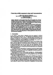
To demonstrate the effectiveness of the quality index, Figure 1 shows the a 2-dimentional simulation example consisting of 4 clusters and its total quality index where the outliers are clearly far away from the main data cloud. The true percentage of outliers is 10%. The simulation runs with the number of 4

4

−5

Quality Index

0

5

10

50

●● ● ●● ●● ●● ● ● ● ●● ●● ● ● ● ● ● ● ● ● ● ● ● ● ● ● ● ● ● ● ● ● ● ● ● ● ● ● ● ● ● ● ● ● ● ● ● ●● ● ● ● ● ● ● ● ● ● ● ● ● ● ● ● ● ● ● ● ● ● ● ● ● ● ● ● ● ● ● ● ● ● ● ● ● ● ● ● ● ● ● ● ● ● ● ● ● ● ● ● ● ● ● ● ● ● ● ● ● ● ●● ● ● ● ● ● ● ● ● ● ● ● ● ● ● ●● ● ● ● ● ● ● ● ● ● ● ● ● ● ● ● ● ● ● ● ● ● ●● ● ● ● ● ● ● ● ● ● ● ● ● ● ● ● ● ● ● ● ● ● ● ● ● ● ● ● ● ● ● ● ● ● ●● ● ● ●● ●● ● ● ●● ● ●● ●● ●● ● ● ● ● ● ●● ● ● ● ● ● ● ● ● ● ●● ● ● ● ● ●● ● ●● ● ● ● ● ● ● ● ● ● ● ● ● ● ● ● ● ● ● ● ● ● ● ● ● ● ● ● ● ● ● ● ● ● ● ● ● ● ● ● ● ● ● ● ● ● ● ● ● ● ● ● ● ● ● ● ● ● ● ● ● ● ● ● ● ● ● ● ● ● ● ● ● ● ● ● ● ● ● ● ● ● ● ● ● ● ● ● ●● ● ● ● ● ● ● ● ● ● ● ● ● ● ● ● ● ● ● ● ● ● ● ●● ● ● ● ● ● ●● ● ● ● ● ● ● ● ● ● ● ● ● ● ● ● ● ● ● ● ● ● ● ● ● ● ● ● ● ● ● ● ● ● ● ●● ● ● ● ● ● ● ● ● ● ● ● ● ● ● ● ● ● ● ● ● ● ● ● ● ● ● ● ● ● ● ● ● ● ● ● ● ● ● ● ● ● ● ● ● ● ● ● ● ● ● ● ● ● ● ● ● ● ● ● ● ● ● ●● ● ● ●● ● ● ● ● ● ● ●● ● ● ● ● ● ● ● ● ● ● ● ● ● ● ● ●● ● ●● ● ● ● ● ● ● ● ● ● ● ● ● ● ● ● ● ● ● ● ● ● ●●●● ● ● ●● ● ●

0

10 0

5

X[,2]

● ● ●●● ● ● ● ● ● ●● ● ● ● ● ● ● ● ● ● ● ● ● ● ● ● ● ● ● ● ● ● ● ● ● ● ● ● ● ● ●● ● ● ● ●● ● ● ● ● ● ●● ● ● ● ● ● ● ● ● ● ● ● ● ● ●● ● ● ● ● ● ● ● ● ● ● ● ● ● ● ● ● ● ● ● ● ● ● ● ● ● ● ● ● ● ● ● ● ● ●● ● ● ● ● ● ● ● ● ● ● ● ●● ● ● ● ● ● ● ● ● ● ● ● ●● ● ● ● ● ●● ● ● ● ● ● ● ●● ● ● ● ● ● ●●● ●● ● ● ● ● ● ● ● ●● ● ●●

100

150

4

15

20

●● ● ●●● ● ● ● ●●● ● ● ● ●● ● ● ● ●● ● ● ● ● ● ●● ● ● ● ● ● ●● ● ● ● ● ● ●● ● ●●● ●● ●● ● ● ●●● ● ● ● ● ● ● ●● ● ● ● ● ●●● ● ● ● ● ●●● ● ● ● ● ● ●● ● ●● ●● ● ● ● ● ● ●

15

20

4 5

5 45 5 44 54 55 444 3 5 55 45 44 3 3 3 3 3 3 3 3 33 33332222 2 2 32 222222222 2 5 455 35 4 3 4 4 3 25 25 0.1

X[,1]

4 5

5

4 5

0.2

0.3

5 5 5 45 45 4444 3333 33

222222

0.4

0.5

ALPHA

(a) Raw Data

(b) Quality Index

Figure 1: A Simulation Example with Outliers far away from the Four Clusters clusters from 2 to 6. α represents the trimming percentage in the above algorithm. It is easy to see that, there is a significant jump when α = 0.1 if 4 clusters are specified. If α < 0.1, since the outliers are far from any clusters, its distance from the data center dominates the quality index. When α > 0.1, some “good” data points are screened out as “outliers”, however, their impact of the total quality index is marginal. When different number of clusters was specified, the quality index has a significant pattern. For example, if G < 4, there is sharp significant spike in 10% and the quality index cycles as α gets bigger. If G > 4, although there is a significant spike in 10%, the quality curve is approximately the same as that when G = 4. Due to the complexity imposed by more clusters, a small size of clusters is always preferred. Although the above simulation example shows a clear cut of the right trimming percentage given an appropriate number of clusters, when outliers are very close to the main data cloud, quality index may change differently. To illustrate this point, Figure 2 shows the same 4 clusters where outliers are quite close to these clusters. In this case, when G = 4, it is found that the quality index curve is monotonely decreasing as α gets bigger. There is no clear cut off at around 10%, however, the curve change does get slower after α = 0.1. The same is true for G > 4 and similar to G = 4. On the other hand, when G < 4, the cyclic pattern still appears when α gets bigger. This clearly indicates that G = 4 is an appropriate selection of cluster numbers and α should be around 10%. Due to the limited space, the application of the data quality assessment framework in a real example is omitted here. Interested readers may refer to Duan et al. (2007) for detailed discussions.

5

Conclusions and Discussions

Although data mining is popularly used in business and industry to improve the quality of decision making, data quality is long time ignored in many practices so that the analytical results derived by data mining methods are usually questionable and unreliable to represent useful knowledge and aid decision making. This paper proposed a generic framework for data quality assessment in nonhomogeneous environments based on robust clustering analysis. In particular, trimmed clustering methods are proposed to robustly characterize groups of similar observations and trimmed observations are then evaluated to assess outlying-ness based on their distance with the cluster profiles. The key of the proposed framework is the determination of appropriate trimming probability and 5

●

●

12 10

●

2

●

−10

●

−5

0

5

2

10

2 3 333 33 2 33 3 2 3 3 2 3 2 2 3 222222

8 4

0 −5

X[,2]

●

6

●

● ● ●●● ●● ●● ●● ● ● ● ● ●● ● ● ●● ● ● ● ● ●●● ● ● ●● ●● ● ● ● ●●● ● ●● ● ● ● ●●●● ● ● ● ● ● ● ● ● ● ● ● ● ● ● ● ● ● ● ● ● ● ● ● ●●● ● ● ● ● ● ● ● ● ● ● ● ● ● ●● ●●●● ● ● ● ● ● ● ●● ● ● ● ● ● ● ● ● ● ●● ● ● ● ● ● ● ● ● ● ● ● ● ● ● ● ● ● ● ● ● ● ● ● ● ● ● ● ● ● ● ●● ● ● ● ●● ● ● ●● ● ● ● ● ● ● ● ● ● ● ● ● ● ● ● ●● ● ● ●● ● ● ● ● ● ● ● ●● ●● ● ●● ● ●● ● ● ● ● ●● ● ● ● ● ● ● ●● ● ● ● ● ● ● ● ●● ● ● ● ●● ● ● ● ●● ● ●●● ● ● ●● ● ●● ●● ● ● ● ●● ●● ● ● ●●● ● ● ● ●● ●● ● ●● ● ● ● ● ●● ● ● ● ● ● ●● ● ● ● ● ● ● ● ● ● ● ● ● ● ● ● ● ● ● ● ● ●● ● ● ● ● ●● ●● ●● ● ● ● ● ● ● ● ● ● ● ● ● ● ● ● ●● ● ●● ● ● ● ● ● ● ● ● ● ● ● ● ● ● ● ●● ● ● ● ● ● ● ● ● ● ● ● ● ● ● ● ● ●● ● ● ● ●● ● ● ● ● ● ● ● ● ● ● ● ●● ● ● ● ● ● ● ● ● ● ● ●●● ● ● ● ● ● ● ● ● ●● ● ● ● ● ● ● ● ●● ● ● ● ● ● ● ● ● ●● ● ● ● ● ● ● ● ● ● ● ● ● ● ●● ● ● ●● ● ●● ● ●● ● ● ● ● ● ● ● ● ● ● ● ● ● ● ● ● ● ● ● ● ● ● ● ● ● ● ● ● ● ● ● ● ● ● ● ●● ●● ● ● ● ● ● ● ● ● ● ● ● ● ● ● ● ● ● ● ● ● ● ● ●● ●● ● ●● ● ● ● ● ● ● ● ● ● ● ● ● ● ●●● ● ● ● ● ●● ● ● ● ● ● ● ● ● ● ● ● ●● ● ● ● ● ●● ● ● ● ● ● ● ● ● ● ● ● ● ● ● ● ● ● ● ● ● ● ● ● ● ●● ● ● ● ● ● ● ● ● ● ● ● ● ● ●● ●● ● ● ●● ● ● ●● ● ●● ● ● ●● ● ● ● ● ● ● ● ● ● ●● ● ● ●● ● ● ●● ●● ● ● ● ● ● ● ●● ● ● ● ● ●● ●●●●● ● ● ● ● ● ● ● ● ● ● ● ● ● ● ● ● ● ● ● ● ● ● ● ●● ● ● ●

Quality Index

10 5

● ● ●● ● ●● ● ●●● ● ● ● ● ● ● ● ●● ● ● ● ●●● ● ● ● ● ●● ● ● ● ● ●● ● ● ● ● ● ●● ● ● ●●●● ● ● ● ● ●●● ● ● ● ● ● ● ●● ● ● ● ●● ● ● ●● ● ● ● ● ● ● ● ● ● ● ● ●●● ● ● ● ● ● ● ● ● ●● ● ● ● ● ● ● ● ● ● ● ● ● ● ● ● ● ● ● ● ● ● ● ●● ● ● ● ● ●● ●● ● ● ● ● ● ● ● ●●● ● ● ● ●● ● ● ● ● ● ● ● ● ●●● ● ● ● ●● ● ● ● ● ● ● ● ● ● ●●● ● ● ●● ● ● ● ● ● ● ●●● ● ● ●● ●● ● ● ● ● ● ● ● ● ● ●

4 54 6 2 354 6 2544 3 32 22 65 2 25 23 24 24 43 44 36 36 5 33 35 6 65 65 65 6 0.1

X[,1]

2 3 3 2 44 4444444444444 65 55 6 65 55 65 55 55 65 65 6 66 65 66 65 66

0.2

0.3

0.4

0.5

ALPHA

(a) Raw Data

(b) Quality Index

Figure 2: Another Simulation Example with Outliers close to the Four Clusters cluster numbers. Even though many criteria have been proposed to select cluster numbers such as BIC, there is little work addressing the trimming probability. The proposed framework defines total quality index as a metric to assess quality induced by number of clusters and trimming probability. The simulation study has shown the effectiveness of this metric in terms of determining these parameters. Extensions of the present work can be made using more rigorous criteria such as BIC. This will be further pursued in the future.

References [1] Barnett, V. and Lewis, T. (1994), Outliers in Statistical Data, 3rd Edition, Wiley, Chichester. [2] Deming W. E. (1994), The New Economics for Industry, Government, and Education (2nd edition). MIT Center for Advanced Engineering Study, Cambridge, Massachusetts, USA. [3] Duan, R., Au, T., and Jiang, W. (2007), “A Data Quality Assessment Framework based on Robust Clustering, Manuscript. [4] English, L. P. (1999), Improving Data Warehouse and Business Information Quality: Methods for Reducing Costs and Increasing Profits. John Wiley & Sons, New York. [5] Fayyad, U., Piatetsky-Shapiro, G., and Smyth, P. (1996), “From Data Mining to Knowledge Discovery in Databases, AI Magazine, 17 (3). [6] Fraley, F. and Raftery, A. E.(2002), “Model-based clustering, discriminant analysis, and density estimation,” Jounral of the American Statistical Association, 97, 611-631. [7] Garcia-Escudero, L. A. and Gordaliza, A. (1999), “Robustnes Properties of k-Means and Trimmed k-Means, Journal of American Statistical Association, 94, 956-969. [8] Garcia-Escudero, L. A., Gordaliza, A. and Matran, C. (2003), “Trimming Tools in Exploratory Data Analysis, Journal of Computational and Graphical Statistics, 12, 434-449. [9] Gallegos, M. T. Ritter, G. (2005), “A Robust Method for Cluster Analysis, Annals of Statistics, 33, 347-380. 6

[10] Hartigan, J. A. (1975), Clustering Algorithms, Wiley, New York. [11] Hastie, T., Tibshirani, R. and Friedman, J. (2001), The Elements of Statistical Learning, New York: Springer. [12] Juran, J. M. (1999), Jurans Quality Handbook. 5th ed. McGraw-Hill. [13] McDonald, G. C. (1994), “Adjusting for Data Contamination in Statistical Inference, Journal of Quality Technology, 26(2), 88-95. [14] Qian, Z., Jiang, W. and Tsui, K-L (2006), “Churn Detection via Customer Profile Modeling”, International Journal of Production Research, . [15] Redman, T. C. (1998), “The Impact of Poor Data Quality on the Typical Enterprise, Communications of ACM, 41(2), 79-82. [16] Rousseeuw, P. J. and Van Driessen, K. (1999), “A Fast Algorithm for the Minimum Covariance Determinant Estimator”, Technometrics, 41, 212-223. [17] TDWI (2002), Data Quality and the Bottom Line: through a Commitment to High Quality Data. The http://www.dw-institute.com/research/display.asp?id=6064.

7

Achieving Business Success Data Warehousing Institute,