classification of liss iv imagery using decision tree methods

The International Archives of the Photogrammetry, Remote Sensing and Spatial Information Sciences, Volume XLI-B8, 2016 XXIII ISPRS Congress, 12–19 July 2016, Prague, Czech Republic

CLASSIFICATION OF LISS IV IMAGERY USING DECISION TREE METHODS Amit Kumar Verma a, *,P.K Garg b, K.S Hari Prasad b, V.K Dadhwal c a

b

Research Scholar, Geomatics Engineering Group, IIT Roorkee, Roorkee-247667, India - [email protected] Professor, Civil Engineering Department, IIT Roorkee, Roorkee-247667, India - (gargpfce, suryafce)@iitr.ernet.in c Director, National Remote Sensing Centre, ISRO, Hyderabad-500042, India - [email protected] Commission VIII, WG VIII/8

KEY WORDS: Crop, Vegetation Indices, Texture, Decision Tree, Classification, LISS IV

ABSTRACT: Image classification is a compulsory step in any remote sensing research . Classification uses the spectral information represented by the digital numbers in one or more spectral bands and attempts to classify each individual pixel based on this spectral information. Crop classification is the main concern of remote sensing applications for developing sustainable agriculture system. Vegetation indices computed from satellite images gives a good indication of the presence of vegetation. It is an indicator that describes the greenness, density and health of vegetation. Texture is also an important characteristics which is used to identifying objects or region of interest is an image. This paper illustrate the use of decision tree method to classify the land in to crop land and non-crop land and to classify different crops. In this paper we evaluate the possibility of crop classification using an integrated approach methods based on texture property with different vegetation indices for single date LISS IV sensor 5.8 meter high spatial resolution data. Eleven vegetation indices (NDVI, DVI, GEMI, GNDVI, MSAVI2, NDWI, NG, NR, NNIR, OSAVI and VI green) has been generated using green, red and NIR band and then image is classified using decision tree method. The other approach is used integration of texture feature (mean, variance, kurtosis and skewness) with these vegetation indices. A comparison has been done between these two methods. The results indicate that inclusion of textural feature with vegetation indices can be effectively implemented to produce classified maps with 8.33% higher accuracy for Indian satellite IRS-P6, LISS IV sensor images.

1. INTRODUCTION Classification of satellite imagery plays an important role in many application of remote sensing. Classification is a method by which labels or class identifiers are attached to the pixels making up remotely sensed image on the basis of their spectral characteristics. These characteristics are generally measurements of their spectral response in different wavebands. They also include other attributes (e.g. Vegetation indices and Texture). Spectral vegetation indices in remote sensing have been widely used for the assessment and analysis of the biomass, water, plant and crops (Jackson and Huete, 1991). Vegetation indices (VI) enhances the spectral information and increases the separability of the classes of interest therefore it influences the quality of the information derived from the remotely sensed data. Texture is also one of the important characteristics used in identifying objects or region in an image. It is an innate property of virtually all surfaces which includes the pattern of different crops in a field. Texture contains important information about the structural arrangement of surfaces and their relationship to surrounding environment. In pixel-based approach, each pixel is classified individually, without considering contextual information. Several studies have explored the potential for using these texture statistics derived from satellite imagery as input features for land cover classification (Haralick et al, 1973, Harris, 1980, Shih et al, 1983).

traditional hard classification techniques are parametric in nature and they expect data to follow a Gaussian distribution, they have been found to be performing poor results. In order to overcome this problem, non-parametric classification techniques such as artificial neural network (ANN) and Decision tree classification (DT) are used. The non-parametric property means that non homogenous, non-normal and noisy data sets can be handled, as well as non-linear relations between features and classes, missing values, and both numeric and categorical inputs (Quinlan, 1993). Decision tree technique includes a set of binary rules that define meaningful classes to be associated to individual pixels. Different decision tree software are available to generate binary rules. The software takes training set and supplementary data to define effective rules. In this study decision tree approach is used for land cover studies using LISS IV sensor data.

2. THE STUDY AREA The selected area for this study is village Foloda which is located in Muzaffarnagar District, India, Measuring approximately 8 km2 which lies between 29°36'22.70"N - 29°38'41.11"N Latitude and 77°47'50.26"E - 77°50'38.21"E Longitude. The ground truth information of the study area, including field wise information of various crops and non-crop were collected using Trimble JUNO Global Positing System (GPS).The main crop growing in this region are sorghum, paddy, wheat and sugarcane. The study area is shown in Figure 1.

Many algorithms have been developed and tested to classify satellite images. There are two approaches namely supervised and unsupervised classification, known as hard classifiers. The * Corresponding author

This contribution has been peer-reviewed. doi:10.5194/isprsarchives-XLI-B8-1061-2016

1061


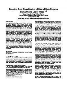
4. METHODOLOGY 4.1 Data Pre-processing Satellite based multispectral imagery contains various quantitative information related to surface and atmosphere. The procedure of retrieving surface reflectance or removing atmospheric contamination from satellite measured radiance is called atmospheric correction. To extract the accurate information about surface we need to correct atmospheric influence. In this study atmospheric correction is done by SACRS2 (Scheme for Atmospheric Correction of Resoursat-2 Sensor), which is developed by Space Application Centre (SAC), Ahmedabad, India. SACRS2 is based on the parameterization of the equations describing radiative transfer model in the atmosphere. It is a GUI based atmospheric correction model developed using signal simulations by the radiative transfer model 6SV-code (Vermote et al., 2006). The GUI of SACRS2 and flow diagram of atmospheric correction is shown in Figure 3 and Figure 4 respectively.

Figure 1. The study area

3. SATELLITE DATA USED Crop classification during Kharif season using satellite data is generally hampered due to the cloud cover problem. Because of the cloudy days, completely cloud free data set of Resourcesat- 2 (IRS-P6) was not available from July to October. Indian satellite IRS-P6, LISS-IV sensor data (Path 96, Row 50) of September 15, 2013 imagery has been taken for this work. The LISS-IV sensor has three band in different region of EMR (b2: Green, b3: Red, b4: NIR). The satellite image of LISS IV sensor is shown in Figure 2 and the details of LISS-IV data is shown in Table 1.

Figure 3. Atmospheric correction SACRS2 model

LISS IV Sensor DN Raw Data

Input Stack (Green, Red and NIR) Figure 2. False colour composite image

Spectral Bands (nm)

Swath Width

Spatial Resolution

Radiometric Resolution

70/23 Km

5.8 meter

10 bit

SACRS2 MODEL For Atmospheric Correction

Lmin, Lmax , Julian Date, Viewing Geometry, Atmospheric Inputs (AOT, WV, O3 etc)

b2 : 520-590

TOA Reflectance b3 : 620-680 b4: 770-860

Surface Reflectance

Figure 4. Flow diagram of atmospheric correction

Table 1. LISS-IV sensor data specification


1062


4.2 Generation of Various Vegetation Indices Various vegetation indices have been developed by linear combination of red, green and near-infrared spectral bands (Basso et al., 2004). Vegetation indices are more sensitive than the individual bands to vegetation parameters (Baret and Guyot, 1991). The eleven vegetation indices Normalized Green (NG), Normalized Red (NR), Normalized Near Infrared (NNIR), Vegetation Index Green (VI green), Difference Vegetation Index (DVI), Normalized Difference Vegetation Index (NDVI), Green Normalized Difference Vegetation Index (GNDVI), Normalized Difference Water Index (NDWI) Optimized Soil Adjusted Vegetation Index (OSAVI), Modified Soil Adjusted Vegetation Spectral Index (MSAVI2) and Global Environmental Monitoring Index (GEMI) are generated using reflectance of green, red and NIR bands of LISS IV sensor. ENVI 5.1 band math function is used for formulation of vegetation indices. The different formulae of vegetation indices are shown by equations (1)-(11) and generated images is shown in Figure 5.

NG  NR 

 green

(1)

 green  red  nir red  green  red  nir

NNIR 

(2)

nir  green  red  nir  green  red

(3)

VIgreen 

(4)

 green  red DVI   nir   red   red NDVI  nir nir  red nir   green

GNDVI  NDWI 

(5) 4.3 Generation of Various Texture Images (6)

(7)

nir   green

 green  nir

(8)

 green  nir

nir  red OSAVI  (1  L) (Where L= 0.16) (9) nir  red  L MSAVI2  (2* nir  1  (2* nir  1) 2  8*( nir  red ) 2    0.125  GEMI   (1  0.25 )   red   1  red )  Where  

Figure 5. Generated vegetation indices images

(10)

(11)

[2*(  2nir   2red )  1.5nir  0.5red ] nir  red  0.5

[Eq. 1: (Sripada et al., 2006); Eq. 2: (Sripada et al., 2006); Eq. 3: (Sripada et al., 2006); Eq. 4: (Gitelson et al., 2002); Eq. 5: (Tucker, 1979); Eq. 6: (Rouse et al., 1974); Eq. 7: (Buschmann and Nagel, 1993); Eq. 8: (McFeeters, 1996); Eq. 9: (Rondeaux et al., 1996); Eq. 10: (Qi et al., 1994); Eq. 11: (Pinty and Verstraete, 1992)]

Image is a function f(x,y) of two space variables x and y, x=0,1,…..,N-1 and y=0,1,……, M-1. The function f(x,y) can take discrete values i=0,1,…..,G-1, where G is the total number of intensity levels in the image. The intensity level histogram is a function showing the number of pixels in the whole image, which have this intensity: N 1 M 1

h(i) 

  ( f ( x, y), i)

(12)

x 0 y 0

Dividing the values h (i) by total number of pixels in the image one obtain the approximate probability density of the intensity levels

p(i )  h(i ) / NM , i  0,1,......G  1

(13)

Different useful image parameters can be worked out from the histogram to quantitatively describe the first-order statistical properties of the image. Most often the so-called central moments (Papoulis 1965) are derived from it to characterize the texture (Levine 1985, Pratt 1991), as defined by Equations (14)-(17) below and the generated texture images is shown in Figure 6.

Mean(  ) 

G 1

 ip(i)

(14)

i 0


1063


Variance( 2 ) 

G 1



(i   )2 p(i)

(15)

i 0

Skewness( 3 )  

3

G 1

 (i  )

3

p(i)

(16)

i 0

Kurtosis( 4 )   4

G 1

 (i )

4

p(i)  3

(17)

i 0

Figure 6. Generated texture images

4.4 Decision Tree Classification The decision tree is an approach where pixels are classified based on a sequence of binary decisions (Safavian and Landgrebe, 1991). According to decision tree, the first conditional statement leads to the second, the second to the third and so on. Decision tree is an inductive learning algorithms which generates classification tree using the training samples. MATLAB 15a was used to build decision trees. In this study training samples are selected based on Google Earth and GPS field observations. The characteristics of training sample ROIs is summarize in Table 2. Number of ROIs

Number of pixels

Water

11

203

Fallow

16

320

Settlement

9

272

Poplar Tree

12

237

Orchard

9

210

Sugarcane

21

421

Paddy

16

252

Sorghum

7

203

Table 2. Number of ROIs and Pixels in each class

4.4.1 Decision tree classification based on vegetation indices: The steps used in this classification are given below: Node 1: if VIgreen < 0.0971 then node 2 else if VIgreen >= 0.0971 then node 3 else class fallow Node 2: if DVI < 0.0303 then node 4 else if DVI >=0.0303 then node 5 else class fallow Node 3: if NNIR < 0.642 then node 6 else if NNIR >= 0.642 then node 7 else class orchard Node 4: class = settlement Node 5: if NR < 0.297 then node 8 else if NR >= 0.297 then node 9 else fallow Node 6: class = water Node 7: if GEMI < 0.302 then node 10 else if GEMI >= 0.302 then node 11 else orchard Node 8: if MSAVI2 < 0.0597 then node 12 else if MSAVI2 >= 0.0597 then node 13 else sorghum Node 9: class = fallow Node 10: class = poplar tree Node 11: if NDVI < 0.586 then node 14 else if NDVI >= 0.586 then node 15 else orchard Node 12: if DVI < 0.0386 then node 16 else if DVI >= 0.0386 then node 17 else sugarcane Node 13: class = sorghum Node 14: if OSAVI< 0.198 then node 18 else if OSAVI >= 0.198 then node 19 else sugarcane Node 15: if GEMI= 0.3042 then node 21 else orchard Node 16: class = sorghum Node 17: class = fallow Node 18: class = orchard Node 19: if DVI < 0.0439 then node 22 else if DVI >= 0.0439 then node 23 else sugarcane Node 20: if NG < 0.252 then node 24 else if NG >= 0.252 then node 25 else orchard Node 21: if NDWI < -0.416 then node 26 else if NDWI >= - 0.416 then node 27 else other crops Node 22: if DVI < 0.0422 then node 28 else if DVI >= 0.0422 then node 29 else sugarcane Node 23: if GNDVI < 0.377 then node 30 else if GNDVI >= 0.377 then node 31 else sugarcane Node 24: class = poplar tree Node 25: class = orchard Node 26: class = orchard Node 27: class = paddy Node 28: class = paddy Node 29: class = sugarcane Node 30: class = orchard Node 31: if NDWI < -0.383 then node 32 else if NDWI >= - 0.383 then node 33 else sugarcane Node 32: class = sugarcane Node 33: if DVI < 0.044 then node 34 else if DVI >= 0.044 then node 35 else sugarcane Node 34: class = sugarcane Node 35: class = paddy 4.4.2 Decision tree classification based on vegetation indices and textural features: The steps used in this classification are given below: Node 1: if GEMI < 0.274 then node 2 else if GEMI >= 0.274 then node 3 else 1 Node 2: if NR < 0.272 then node 4 else if NR >= 0.272 then node 5 else 5 Node 3: if VIgreen < 0.0841 then node 6 else if VIgreen >=0.0841 then node 7 else 1 Node 4: class = water


1064


Node 5: class = settlement Node 6: if NDVI < 0.264 then node 8 else if NDVI >= 0.264 then node 9 else 1 Node 7: if GEMI < 0.294 then node 10 else if GEMI >= 0.294 then node 11 else 7 Node 8: class = fallow Node 9: if kurtosis < 1.595 then node 12 else if Kurtosis >=1.595 then node 13 else 6 Node 10: if mean < 0.0022 then node 14 else if Mean >= 0.0022 then node 15 else 4 Node 11: if NDVI < 0.490 then node 16 else if NDVI >= 0.490 then node 17 else 3 Node 12: class = sorghum Node 13: class = fallow Node 14: if NDVI < 0.461 then node 18 else if NDVI >= 0.461 then node 19 else 4 Node 15: class = orchard Node 16: if skewness < 0.0011080 then node 20 else if Skewness >= 0.0011080 then node 21 else 7 Node 17: if DVI < 0.046901 then node 22 else if DVI >= 0.046901 then node 23 else 2 Node 18: class = orchard Node 19: class = poplar tree Node 20: if skewness < -0.0001811 then node 24 else if Skewness = -0.0001811 then node 25 else 7 Node 21: class = paddy Node 22: if GNDVI < 0.401 then node 26 else if GNDVI >= 0.401 then node 27 else 2 Node 23: if GDVI < 0.0420 then node 28 else if GDVI >= 0.0420 then node 29 else 3 Node 24: class = paddy Node 25: if variance < 5.59059e-06 then node 30 else if Variance >= 5.59059e-06 then node 31 else 7 Node 26: class = orchard Node 27: class = poplar tree Node 28: class = paddy Node 29: class = orchard Node 30: class = sugarcane Node 31: class = orchard

Orchard

83.54

86.71

89.54

88.91

Sugarcane

82.64

78.18

85.17

88.46

Paddy

71.25

81.71

81.44

79.83

Sorghum

77.94

75.17

79.18

82.31

OA= 81.09 K=0.79

OA= 89.42 K= 0.87

Table 3. Classification accuracy

5. RESULTS AND CONCLUSIONS The final classified images are shown in Figure 7 and Figure 8.

Figure 7. Classified image using decision tree (VI)

4.5 Accuracy Assessment Accuracy assessment is used to compare the classification results with reference data, which is assumed to be true for determining the classification results. Many methods are used to analyse the accuracy of remotely sensed data (Congalton and Green, 1999, Koukoulas and Blackburn, 2001). In this work, confusion matrix or error matrix method is used (Foody, 2002). Reference data has been taken during the field visit on September 18-21, 2013. Total 650 pixels have been selected for various classes to determine the accuracy. The accuracy assessment has been done using ERDAS IMAGINE software. The producer’s accuracy (PA), user’s accuracy (UA), overall accuracy (OA) and kappa coefficient (K) values are given in Table 3. Class Name

DT ( VI)

DT (VI + Texture)

PA

UA

PA

UA

Water

91.31

84.54

96.21

92.91

Fallow

87.64

81.28

95.82

92.48

Settlement

92.18

89.71

97.71

96.23

Poplar Tree

82.17

84.54

91.64

89.32

Figure 8. Classified image using decision tree (VI & Texture)


1065


Indian satellite IRS-P6 LISS IV sensor imagery has been classified using decision tree method. The first decision tree was constructed based on only vegetation indices and the second one was constructed using vegetation indices with textural features. The final image was classified into eight major classes (water, fallow, settlement, poplar tree, orchard, sugarcane, paddy and sorghum). The overall accuracy and kappa coefficient is found to be 81.08 % and 0.79 for decision tree using vegetation indices method. Inclusion of textural feature with vegetation indices decision tree, overall accuracy and kappa coefficient is 89.42 % and 0.87 respectively. The results indicates that LISS IV imagery can be effectively implemented to produce classified maps with higher accuracy. ACKNOWLEDGEMENTS

The authors are thankful to Indian Institute of Technology Roorkee for providing software’s for the study (ENVI 5.1, ARCGIS 10.2.1, MATLAB 2015a and JUNO GPS) and the farmers for providing necessary information and support during the field visit.

Levine, M., 1985. Vision in Man and Machine, McGraw-Hill. McFeeters, S. K., 1996. The use of normalized difference water index (NDWI) in the delineation of open water features. International Journal of Remote Sensing (17), pp. 1425–1432. Papoulis, A., 1965. Probability, Random Variables and Stochastic Processes, McGraw-Hill. Pinty, B. and Verstraete, M. M., 1992. GEMI: a non-linear index to monitor global vegetation from satellites. Vegetatio (101), pp. 15–20. Pratt, W., 1991. Digital Image Processing, Wiley. Rondeaux, G., Steven, M. and Baret, F., 1996. Optimization of soil-adjusted vegetation indices. Remote Sensing of Environment (55), pp. 95–107. Rouse, J. W., Haas, R. H., Schell, J. A. and Deering, D. W., 1974. Monitoring vegetation systems in the Great Plains with ERTS NASA Goddard space Flight Centre 3d ERTS-1 Symposium, pp. 309-317. Safavian, R. S. and Landgrebe, D., 1991. A survey of decision tree classifier methodology. IEEE Transactions on Systems Man and Cybernetics (21), pp. 660–674.

REFERENCES Baret F. and Guyot G., 1991. Potentials and limits of vegetation indices for LAI and APAR assessment. Remote Sensing of Environment (35), pp.161–173. Basso, B., Cammarano D and De Vita, P., 2004. Remotely sensed vegetation indices: Theory and applications for crop management. Italian Journal of Agrometeorology (53), pp. 36– 53. Buschmann, C., Nagel E., 1993. In vivo spectroscopy and internal optics of leaves as basis for remote sensing of vegetation. International Journal of Remote Sensing (14), pp. 711–722. Congalton, R. G., and Green, K., 1999. Assessing the accuracy of remotely sensed data: principles and practices, Lewis Publishers, Boca Raton. Foody, G. M., 2002. Status of land cover classification accuracy assessment, Remote Sensing of Environment (80), pp. 185201.

Shih, E. H. H., and Schowengerdt, R. A., 1983. Classification of Arid Geomorphic Surfaces using Landsat Spectral and Textural Feature, Photogrammetric Engineering and Remote Sensing 49(3), pp. 337-347. Sripada, R. P., Heiniger, R. W., White, J. G., Meijer, A. D., 2006. Aerial colour infrared photography for determining early inseason nitrogen requirements in corn. Agronomy Journal (98), pp. 968–977. Tucker, C. J., 1979. Red and photographic infrared linear combinations for monitoring vegetation. Remote Sensing of Environment (8), pp. 127–150. Vermote, E., Tanré, D., Deuzé, J. L., Herman M., Morcrette J. J., and Kotchenova, S. Y., 2006. 6S User Guide on Second Simulation of a Satellite Signal in the Solar Spectrum -Vector (6SV), Version 3.

Gitelson, A., Kaufman Y. J., Stark, R., and Rundquist, D., 2002. Novel algorithms for remote estimation of vegetation fraction. Remote Sensing of Environment (80), pp. 76–87. Haralick, R.M., K.Shanmugam and I.Dinstein., 1973. Textural Features for Image Classification, IEEE Transactions on Systems Man and Cybernetics, Vol. SMC-3: pp. 610- 621. Harris, R., 1980. Spectral and Spatial Image Processing for Remote Sensing, International Journal of Remote Sensing 1(4), pp.361-375. Jackson, R. D., and Huete, A. R., 1991. Interpreting vegetation indices, Preventive Veterinary Medicine 11(3–4), pp. 185-200. Koukoulas, S., and Blackburn, G. A., 2001. Introducing new indices for accuracy evaluation of classified images representing semi-natural woodland environments, Photogrammetric Engineering and Remote Sensing, (67), pp. 499-510.


1066