balancing algorithms for different parallel algorithmic paradigms. Keywords: Load Balancing, Load Matching, Under load,. Over load, processor communication, ...
IJCSI International Journal of Computer Science Issues, Vol. 8, Issue 5, No 1, September 2011 ISSN (Online): 1694-0814 www.IJCSI.org
411
Classification of Load Balancing Conditions for parallel and distributed systems Zubair Khan1
Ravendra Singh2
Jahangir Alam3
Shailesh Saxena4
1,4
Department Of Computer Science and engineering Invertis University Bareilly India
2
Department of CS&IT MJP Rohilkhand University Bareilly, India
3
Woman Polytechnic Department of CSE AMU Aligargh India
Abstract Although intensive work has been done in the area of load balancing, the measure of success of load balancing is the net execution time achieved by applying the load balancing algorithms. This paper deals with the problem of load balancing conditions of parallel and distributed applications. Parallel and distributed computers have multiple-CPU architecture, and in parallel system they have shared memory. While in distributed system each processing element has its own private memory and connected through networks. Parallel and distributed systems communicate to each other by Message-passing mechanism. Based on the study of recent work in the area, we propose a general classification for describing and classifying the growing number of different load balancing conditions. This gives an overview of different algorithms, helping designers to compare and choose the most suitable strategy for a given application .To illustrate the applicability of the classification, different well-known load balancing algorithms are described and classified according to it. Also, the paper discusses the use of the classification to construct the most suitable load balancing algorithms for different parallel algorithmic paradigms. Keywords: Load Balancing, Load Matching, Under load, Over load, processor communication, Network(Topology)
1. Introduction Load balancing is one of the central problems which have to be solved to achieve a high performance from a parallel computer. For parallel applications load balancing attempts to distribute the computation load
across multiple processors or machines as evenly as possible to improve performance. Since load imbalance leads directly to processor idle times, high efficiency can only be achieved if the computational load is evenly balanced among the processors. Generally a load balancing scheme consists of three phases-1.Information collection, 2.Decision-Making and 3.Data migration. 1.1 Information collection: During this phase the load balancer gathers the information of workload distribution and the state of computing environment and detects whether there is a load imbalance. 1.2 Decision-Making: This phase focuses on calculating an optimal data distribution. 1.3 Data migration: This phase transfer the excess amount of workload from overloaded processor to under loaded ones. Three kinds of load balancing schemes have been proposed and reviewed in the literature [2], and they can be distinguished depending on the knowledge about the application behavior. The first one, static load balancing, is used when the computational and communication requirements of a problem are known a priori. In this case, the problem is partitioned into tasks and the assignment of the task-processor is performed once before the parallel application initiates its execution. The second approach, dynamic load balancing schemes, is applied in situations where no priori estimations of load distribution are possible. It is only during the actual program execution that it becomes apparent how much work is being assigned to the individual processor. In order to retain efficiency, the imbalance must be detected and an appropriate
IJCSI International Journal of Computer Science Issues, Vol. 8, Issue 5, No 1, September 2011 ISSN (Online): 1694-0814 www.IJCSI.org
dynamic load balancing strategy must be devised. Some dynamic strategies that use local information in a distributed architecture, have been proposed in the literature. These strategies describe rules for migrating tasks on overloaded processors to under loaded processors in the network of a given topology. In this survey dynamic load balancing techniques (also referred as Resource-Sharing, Resource scheduling, job scheduling, task- migration etc.) in large MIMD multiprocessor systems are also studied. Dynamic load balancing strategies have been shown to be the most critical part of an efficient implementation of various algorithms on large distributed computing systems. A lot of dynamic load balancing strategies have been proposed in the last few years. With this large number of algorithms, it becomes harder for designers to compare and select the most suitable strategy. A load-balancing algorithm must deal with different unbalancing factors, according to the application and to the environment in which it is executed. Unbalancing factors may be static, as in the case of processor heterogeneity, or dynamic. Examples of dynamic
412
unbalancing factors include the unknown computational cost of each task, dynamic task creation, task migration, and variation of available computational resources due to external loads. The third one is hybrid load balancing condition when dynamic and static are merge together and perform to take the advantages of both conditions.
2. The Classification The proposed classification is represented in Fig. 1. In order to define a Load-balancing algorithm completely, the main four sub-strategies (initiation, location, exchange, and selection) have to be defined. The goal of this Classification is to understand load balancing algorithms. This Classification provides a terminology and a framework for describing and classifying different existing load balancing algorithms, facilitating the task of identifying a suitable load balancing strategy. A detailed discussion of the Classification is presented in the following sections:
Load balancing Dynamic Load Balancing
Initiation
Load-Selection
Periodic Event Driven
Sender Initiated
Receiver Initiated
Static Load Balancing
Information-Exchange Load-Balancer Location
Processor Load Decision Matching Matching Making
Local
Communication
Global Topology
Randomized
Uniform
Central
Task Exchange
Local
Golomb recovery
trapezium
Distributed
Synchronous
Global
Figure 1 Grouping of Load Balancing Algorithms.
asynchronous
IJCSI International Journal of Computer Science Issues, Vol. 8, Issue 5, No 1, September 2011 ISSN (Online): 1694-0814 www.IJCSI.org
413
2.1Initiation
2.3 Information exchange
The initiation approach specifies the system, which invokes the load balancing behavior. This may be a episodic or event-driven initiation. Episodic initiation is a timer based initiation in which load information is exchanged every preset time interval. The eventdriven is a usually a load dependent policy based on the observation of the local load. Event-driven strategies are more reactive to load imbalances, while episodic policies are easier to implement. However, episodic policies may result in extra overheads when the loads are balanced.
This specifies the information and load flow through the network. The information used by the dynamic load-balancing algorithm for decision-making can be local information on the processor or gathered from the surrounding neighborhood. The communication policy specifies the connection topology (network) of the processors in the system, by sending the messages to its neighboring processing elements. This network doesn’t have to represent the actual physical topology of the processors. A uniform network indicates a fixed set of neighbors to communicate with, while in a randomized network the processor randomly chooses another processor to exchange information with.
2.2 Load-balancer location This approach specifies the location at which the algorithm itself is executed. The load balancing algorithm is said to be vital if it is executed at a single processor, determining the necessary load transfers and informing the involved processors. Distributed algorithms are further classified as synchronous and asynchronous. A synchronous loadbalancing algorithm must be executed simultaneously at all the participating processors. For asynchronous algorithms, it can be executed at any moment in a given processor, with no dependency on what is being executed at the other processors.
2.4 Load selection The load selection is very vital part of system in which the processing elements decide from which node to exchange load . Apart from that, it specifies the appropriate load items(tasks) to be exchanged. Local averaging represents one of the common techniques. The overloaded processor sends loadpackets to its neighbors until its own load drops to a specific threshold or the average load.
Table 1: Classification of dynamic load balancing algorithms Algorithm
Processor Matching
Load Matching
Communication
Applications
LB Locations
Initiation
SASH
Information exchange Global
Processor that will produce the fastest turn around
Cost function
Randomized Global
independent tasks
Central (dedicated)
Event driven (Shortest execution time)
Dynamic Load Balancing (DLB)
Local/ Global
According to the load balancer
cost function which uses past to predict future N/A
Randomized Global
Independent
Central/ Distributed
Receiver initiated
Randomized Global
Whole programs
Central
Event driven (User)
Least loaded processor in the neighborhood of the receiver
load is sent.
Uniform Local
Independent loops
Central/ Distributed
Receiver initiated
Adjacent processors
Load is distributed over the nodes of the island.
Uniform Local
Independent tasks
Distributed Asynchronous
Receiver initiated
Automatic Heteregene-ous Supercomputing
Global
Direct Neighbor-hood Repeated (DNR)
Local
Neighbor
Local
According to the load balancer
loops
If the load difference exceeds a threshold, a percentage of the
IJCSI International Journal of Computer Science Issues, Vol. 8, Issue 5, No 1, September 2011 ISSN (Online): 1694-0814 www.IJCSI.org
414
Central Algorithm
Global
Match overloaded with idle
Divides the load among the loaded and idle peers
Randomized Global
Independent tasks
Distributed Asynchronous
Periodic
Pre -Computed Sliding
Local
Adjacent processors
Uniform Local
Independent tasks
Distributed Asynchronous
Periodic
Rendez-Vous
Global
Matches most load
An extra step, which calculates the required total number of transfers required, is done before transfer Divides the most loaded with least loaded
Randomized Global
Independent tasks
Distributed Asynchronous
Periodic
Random
Local
Random
Each new task is redistributed randomly
Randomized Global
Independent tasks
Distributed Asynchronous
Periodic
Rake
Local
Adjacent processors
Load above the average workload is transferred to the adjacent processor
Uniform Local
Independent Tasks
Distributed Synchronous
Periodic
Tilling (DN)
Local
Balances processors within same window
Uniform Local
Independent tasks
Distributed Synchronous
Periodic
X-Tilling
Local
Balances processors connected in the hypercube
The load is distributed among processors in the window. The load is distributed among processors in the hypercube
Uniform Global
Independent tasks
Distributed Synchronous
Periodic
3. Categorization of Different Load Balancing Algorithms In this paper we will illustrate how the proposed Classification is capable of classifying diverse loadbalancing algorithms. A number of Dynamic load balancing algorithms are existing for different systems; a small description is presented for each algorithm, followed by a detailed classification.
3.I.
Decision and algorithms[25],[26],[8]
Migration
These algorithms are classified as fallows.
based
3.1.1. Local Decision and Local Migration (LDLM): In this strategy a processor distributes some of his load to its neighbors after each fixed time interval. This is a LDLM because the decision to migrate a load unit is done purely local. The receiver of a load is also a direct neighbor. The balancing is initiated by a processing unit which sends a load unit. We implemented this strategy after x iterations of the simulator y load units are sent to random neighbors. 3. I.2. Direct neighborhood (d-N) : if the local load increased by more than Up percent or decrease by more than Down percent, actual value is broadcasted to direct neighbors. if the load of a
IJCSI International Journal of Computer Science Issues, Vol. 8, Issue 5, No 1, September 2011 ISSN (Online): 1694-0814 www.IJCSI.org
processing element exceeds that of its least neighbor load by more than d percent, then it sends one unit to that neighbor. 3. I.3.Local Decision and Global Migration (LDGM): in this strategy the load units are migrated over the whole network to a randomly chosen processor.
3. I.4.Global Decision and Local Migration (GDLM) :The Gradient Model method discussed above in section 2,was introduces by Lin & Keller [10].it belongs to the group of GDLMr-strategies ,because decisions are based on Gradient information. Gradients are vectors consisting of load respectively, distance information of all processing elements. Which means that each processing element wants to achieve well approximated global state information on network?
3. I.5.Global decision and Global Migration (GDGM) : This method is classified as fallows a) Bidding algorithm: it is also a state controlled algorithm. The number of processing elements able to take load from a processor in state H depends on the distance between these processors. b) Drafting Algorithm: in this a processor can be one of the three states L(low),n(normal),H(high) which represent actual load situation. Each processor maintains a load table which contains the most recent information of the so called”candidate processors”. A candidate processors is a processor from which load may be received. Since the workload of system changes dynamically, X-gradient surface can only be approximated. This is done by the protocol that is used in original gradient model For this we recursively define a pressure function p: V-> {0,……D(G)+1 And the suction function S: V ->{0,……D(G)+1}
3.2 The Random Algorithm [16] Each time an element (task) is created on a processor, it is sent on a randomly selected node anywhere in the system. For each node, the expectation to receive a part of the load is the same regardless of its place in the system.
3.3 The Tiling (Direct Neighborhood DN) Algorithm [13] It divides the system in small and disjointed subdomains of processors called windows. A perfect load balancing is realized in each window using regular communications. In order to propagate the work over the entire system, the window is shifted (slightly moved so that they overlap only a part of the old domain) for the next balancing phase.
3.4 The X-Tiling Algorithm [13]
Similar to Tiling algorithm but extra links are added to the current topology of the processor to form a hypercube topology.
3.5 The Rake Algorithm [13] It uses only regular communications with processors in the neighborhood set. Firstly, the average load is processed and broadcasted. In the first transfer phase, during p iterations, each processor sends to its right neighbor the data over the average workload It uses only regular communications with processors in the neighborhood set. Firstly, the average load is processed . In the second transfer phase, during the extra workloads, each processor sends to its right the work over the average workload + 1.
3.6 The Pre-Computed Sliding Algorithm [13] It is an improvement of the Rake algorithm. Instead of transferring data over the average workload of the system, it computes the minimal number of data exchanges needed to balance the load of the system. Unlike the Rake algorithm, it may send data in two directions.
3.7 The Average Neighbor Algorithm [17], [20] The architecture is made of islands. An island is made of a center processor and all the processors in its neighborhood. It works on the load balancing every node in the island. The partial overlapping allows the load to propagate.
3.8 The Direct Neighborhood Repeated Algorithm [21] Once a sender-receiver couple is established, the migrating load can move from the sender to the receiver. In its turn, the receiver can have an even less neighborhood. The receiver is allowed to directly forward the migrating load to the less loaded nodes. Load migration stops when there are no more useful transfers.
3.9 The Central Algorithm [11], [28] Firstly, the average workload is computed and broadcasted to every processor in the system. Then, the processors are classified into 3 classes: idle, overloaded, and the others. The algorithm tries to match each overloaded node with an idle peer.
4. Dynamic Load Balancing (DLB) [18] Synchronization is triggered by the first processor that finishes its portion of the work. This processor then sends an interrupt to all the other active slaves, who then send their performance profiles to the load balancer. Once the load balancer has all the profile information, it calculates a new distribution. If the amount of work to be moved is below a threshold, then work is not moved else a profitability analysis routine is performed. This makes a trade-off between the benefits of moving work to balance load.
415
IJCSI International Journal of Computer Science Issues, Vol. 8, Issue 5, No 1, September 2011 ISSN (Online): 1694-0814 www.IJCSI.org
According to the first run, the application adjusts itself for one of the load balancing strategies: globalcentralized (GCDLB), global-distributed (GDDLB), and local-centralized (LCDLB) and, local-distributed (LDDLB). The compilation phase is used to collect information about the system and generate cost functions, and prepare the suitable libraries to be used after the first run.
4.1. Automatic Supercomputing (AHS) [19]
Heterogeneous
Uses a quasi-dynamic scheduling strategy for minimizing the response time observed by a user when submitting an application program for execution. This system maintains an information file for each program that contains an estimate of the execution time of the program on each of the available machines. When a program is invoked by a user, AHS examines the load on each of the networked machines and executes the program on the machine that it estimates will produce the fastest turn-around time.
4.2. Self-Adjusting Scheduling Heterogeneous Systems (SASH)[20]
for
It utilizes a maximally overlapped scheduling and execution paradigm to schedule a set of independent tasks on to a set of heterogeneous processors. Overlapped scheduling and execution in SASH is accomplished by dedicating a processor to execute the scheduling algorithm. SASH performs repeated scheduling phases in which it generates partial schedules. At the end of each scheduling phase, the scheduling processor places the tasks scheduled in that phase on to the working processors’ local queues. The SASH algorithm is a variation of the family of branch-and-bound algorithms. It searches through a space of all possible partial and complete schedules. The cost function used to estimate the total execution time produced by a given partial schedule consists of cost of executing a task on a processor and the additional communication delay required to transfer any data values needed by this task to the processor. As observed from Table 1, that any dynamic loadbalancing algorithm may be classified according to the Classification. Accordingly, this makes it simpler for designers to compare and select the proper algorithm for their application to be executed on a certain computing environment. The next section will illustrate how to select the most suitable dynamic load-balancing category for the different parallel programming paradigms.
5. Dynamic Load-Balancing Conditions A number of parallel algorithmic paradigms have emerged for parallel computing like:
1. Gradient Model , 2. Sender Initiated Diffusion (SID), 3. Receiver Initiated Diffusion (RID) , 4. Hierarchical Balancing Method (HBM) , 5. The Dimension Exchange Method (DEM) 6. Phase Parallel, 7. Divide and Conquer, 8. Pipeline, 9. Process Farm , Each paradigm has its own characteristics. A brief description is given for each paradigm and a suitable load-balancing algorithm is suggested for each based on the Classification. It should be noted that scalability and low communication cost are the main considerations affecting the choice of the following suggested strategies.
Gradient Model [9] The gradient model is a demand driven approach [8]. The basic concept is that underloaded processors inform other processors in the system of their state, and overloaded processors respond by sending a portion of their load to the nearest lightly loaded processor in the system.
Sender Initiated Diffusion (SID) [15] The SID strategy is a, local, near-neighbor diffusion approach which employs overlapping balancing domains to achieve global balancing. A similar strategy, called Neighborhood Averaging, is proposed in [12]. The scheme is purely distributed and asynchronous. for an N processor system with a total system load L unevenly distributed across the system, a diffusion approach, such as the SID strategy, will eventually cause each processor’s load to converge to L/N.
Receiver Initiated Diffusion (RID) [16] The RID strategy can be thought of as the converse of the SID strategy in that it is a receiver initiated approach as opposed to a sender initiated approach. However, besides the fact that in the RID strategy underloaded processors request load from overloaded neighbors, certain subtle differences exist between the strategies. First, the balancing process is initiated by any processor whose load drops below a prespecified threshold (Llow). Second, upon receipt of a load request, a processor will fulfill the request only up to an amount equal to half of its current load. When a processor’s load drops below the prespecified threshold Llow, the profitability of load balancing is determined by first computing the average load in the domain, Lpavg [(8)]. If a processor’s load is below the average load by more than a prespecified amount, L threshold &, it proceeds to implement the third phase of the load balancing process.
416
IJCSI International Journal of Computer Science Issues, Vol. 8, Issue 5, No 1, September 2011 ISSN (Online): 1694-0814 www.IJCSI.org
Hierarchical [15],[16]
Balancing
Method
(HBM)
The HBM strategy organizes the multicomputer system into a hierarchy of balancing domains, thereby decentralizing the balancing process. Specific processors are designated to control the balancing operations at different levels of the hierarchy.
The Dimension Exchange Method (DEM) [17], [19] The DEM strategy [17], [19] is similar to the HBM scheme in that small domains are balanced first and these then combine to form larger domains until ultimately the entire system is balanced. This differs from the HBM scheme in that it is a synchronized approach, designed for a hypercube system but may be applied to other topologies with some modifications. In the case of an N processor hypercube configuration, balancing is performed iteratively in each of the log N dimensions. All processor pairs in the first dimension, those processors whose addresses differ in only the least significant bit, balance the load between themselves Phase parallel [12]: The parallel program consists of a number of super steps, and each super step has two phases. A computational phase, in which, multiple processes, each perform an independent computation C. In the subsequent interaction phase, the processors perform one or more synchronous interaction operations, such as a barrier or blocking communication. This paradigm is also known as the loosely synchronous paradigm and the a general paradigm. It facilitates debugging and performance analysis, but interaction is not overlapped with computation, and it is difficult to maintain balanced workloads among the processors. Suggested load balancing algorithm: Initiation: event driven, with every synchronization step. Load balancer location: central or distributed synchronous. Information exchange: Decision-making: would be global to observe the different loads. Communication: Global Randomized, as this is the nature of the paradigm. Load selection: processor matching and selection is application dependent.
Fig. 2. Phase Parallel Divide and conquer [12]: In this a problem id divided into small parts and then we start to conquer it. In dynamic load balancing a parent process divides its workload into several smaller pieces and assigns them to a number of child processes. The child processes then compute their workload in parallel and the results are merged by the parent. This paradigm is difficult to maintain balanced workloads among the processors. The parent is the one, which distributes the load among its children, and accordingly it should be the one to balance the load between them. Suggested load balancing algorithm: Initiation: event driven, sender/receiver (child) initiated. Load balancer location: distributed asynchronous. Each parent is responsible to load balance its children. Information exchange: Decision-making: would be local based on the children only. Communication: Local Uniform, as the children can only communicate to parents and their children. Load selection: load is exchanged among the children and selection of load is flexible according to the application.
Fig. 3. Divide and conquer Pipeline [12]: In this the output of one stage works as an input for next stage, hence a pipe is seem to be created called Virtual pipe. A number of processors
417
IJCSI International Journal of Computer Science Issues, Vol. 8, Issue 5, No 1, September 2011 ISSN (Online): 1694-0814 www.IJCSI.org
form a virtual pipe. A continuous data stream is fed into the pipeline and the processes execute at different pipeline stages simultaneously in an overlapped fashion. The pipeline paradigm is the basis for SPMD. Each processor runs the same code with different data. Interface data is exchanged between adjacent processors. Suggested load balancing algorithm: • Initiation: event driven, sender/receiver initiated. • Load balancer location: Central/distributed. Depends on the number of the processors involved in the synchronization. For scalability reasons, a distributed asynchronous strategy is suggested. Information exchange: Decision-making: Global/Local. Local is recommended for scalability. Communication: Local Uniform, as the processors only communicate with their neighbors. Load selection: load is exchanged among the neighbors and selection of load is application dependent.
Process Farm: This is a very common paradigm shown in fig.5. A master process executes the sequential part of the parallel part of the program and spawns a number of slave processes to execute the parallel workload. When a slave finishes its workload, it informs the master which assigns a new workload to the slave. This is a very simple paradigm, but the master could become the bottleneck.
Fig.5. Process farm
Fig.4. Pipe Line
6. Conclusion and Future Work In the paper it has been illustrated how to suggest new algorithms for different application paradigms. The Classification is considered helpful for designers to compare different load-balancing algorithms and design new ones tailored for their needs. In the future, we intend to develop a framework for applications with load balancing that utilizes this Classification and helps the designer tailor his own algorithm. The framework would generate the required libraries needed and the corresponding coding that will facilitate the development of parallel applications.
References [1]M. Willeheek-LeMair and A. P. Reeves, “Region growing on a hyper- cube multiprocessor,” in Proc. 3rd Conf Hypercube Concurrent Comput. and Appl., 1988, pp. 1033- 1042. [2] M. WiIIebeek-LeMair and A. P. Reeves, “A general dynamic load balancing model for parallel computers,” Tech: Rep. EE-CEG-89-I) Cornell School of Electrical Engineering, 1989. [3]T. L. Casavant and .I. G. Kuhl, “A taxonomy of scheduling in general purpose distributed computing systems,” IEEE‘ Trans. Software Eng., vol. 14, no. 2, pp. 141-154, Feb. 1988. [4]Y.-T. Wang and R.I. T. Morris, “Load sharing in distributed systems,” IEEE Trans. Cornput., vol. C-34, pp.
418
IJCSI International Journal of Computer Science Issues, Vol. 8, Issue 5, No 1, September 2011 ISSN (Online): 1694-0814 www.IJCSI.org
204-211, Mar. 1985. M. J. Berger and S. H. Bokhari, “A partitioning strategy for nonuniform problems on multiprocessors,” IEEE Trans. Cornput., vol. C-36, pp. 570-580, May 1987. [5] G. C. Fox, “A review of automatic load balancing and decomposition methods for the hypercube,” California Institute of Technology, C3P- 385, Nov. 1986. [6] K. Ramamritham, I. A. Stankovic, and W. Zhao, “Distributed scheduling of tasks with deadlines and resource requirements,” IEEE Trans. Comput. pp. 11101123, Aug. 1989. [7] K. M. Baumgartner, R. M. Kling, and B. W. Wah, “Implementation of GAMMON: An efficient load balancing strategy for a local computer system,” in Proc. 1989 Int. Conf Parallel Processing, vol. 2, Aug. 1989, pp. 77-80. [8] F. C. H. Lin and R. M. Keller, “The gradient model load balancing method,” IEEE Tran. Software Eng., vol. 13, no. 1, pp. 32-38, Jan. 1987. [9]. Casavant, T. L. and Kuhl, J. G.: A Taxonomy of Scheduling in General-Purpose Distributed Computing Systems. IEEE Trans. on Soft. Eng. 14 (1998) 141-154 [10]. Plastino, A., Ribeiro, C. C. and Rodriguez, N. R.: Load Balancing Algorithms for SPMD Applications. Submitted for publication (2001) [11]. Hillis, W.D.: The Connection Machine. MIT press, 1985. [12]. Fonlupt, C., Marquet, P. and Dekeyser, J.: Dataparallel load-balancing strategies. Parallel Computing 24 (1998) 1665-1684. [13]. Dekeyser, J. L., Fonlupt, C. and Marquet, P.: Analysis of Synchronous Dynamic Load Balancing algorithms”, Parallel Computing: State-of-the Art Perspective (ParCo'95), volume 11 of Advances in Parallel Computing, pages 455--462, Gent, Belgium ( September 1995) [14] V. A. Saletore, “A distrubuted and adaptive dynamic load balancing scheme for parallel processing of mediumgrain tasks,” in Proc. Fifth Distributed kemorycomput. ?onf, Apr. 1990, pp. 995-999. [15] K. G. Shin and Y.-C. Chang, “Load sharing in distributed real time systems with state-change broadcasts,” IEEE Trans. Cornput., pp . 1124-1142, Aug. 1989 .V. A. Saletore, “A distr [16]. Subramanian, R. and Scherson, I.: An Analysis of Diffusive Load Balancing. Proceedings of Sixt h Annual
ACM Symposium on Parallel Algorithms and Architectures, (June 1994) 220-225 [17]. Saletore, V. A.: A distributive and adaptive dynamic load balancing scheme for parallel processing of mediumgrain tasks. Proceedings of the 5th Distributed Memory Conference (April 1990) 995-999 [18] G. Cybenko, “Dynamic load balancing for distributed memory multiprocessors,” J. Parallel and Distributed Comput., vol. 7:279-301, October, 1989. [19]D. P. Bertsekas and J. N. Tsitsiklis, Parallel and Distributed Computation: Numerical Methods. Englewood Cliffs, NJ: Prentice-Hall, [20]. Willebeek- LeMair, M.H. and Reeves, A.P.: Strategies for dynamic load balancing on highly parallel computers. IEEE Trans. on parallel and distributed systems, vol. 4, No. 9 (Sept. 1993) [21]. Corradi, A., Leonardi, L. and Zambonelli, F.: Diffusive load-balancing policies for dynamic applications. IEEE Concurrency Parallel, Distributed and Mobile Computing (January-March 1999) 22-31 [22]. Zaki, M. J., Li, W. and Parthasarathy, S.: Customized dynamic load balancing for a network of workstations. Proceedings of the 5th IEEE Int. Symp., HPDC (1996) 282291 [23]. Dietz, H. G., Cohen, W.E. and Grant, B. K.: Would You Run it Here... or There? (AHS: Automatic Heterogeneous Supercomputing. International Conference on Parallel Processing, Volume II: Software (1993) 217221 [24]. Hamidzadeh, B., Lilja, D. J. and Atif, Y. : Dynamic scheduling techniques for heterogeneous computing systems. Concurrency: Practice and Experience, vol. 7 (1995) 633-652. [25]S.Zhou, A Trace Driven Study Of Load balancing , IEEE Trans.On Software Engineering,Vol.14,no.9,1988,pp,1327-1341. [26]F. Ramme, Lastausgleichsverfahren in Vertileilten Systemen, Master Thesis,University of Paderborn.1990. [27] ] F. C. H. Lin and R. M. Keller, “The gradient model load balancing method,” IEEE Tran. Software Engineering 13, 1987,pp.32-38 [28] Powley, C., Ferguson, C. and Korf, R. E.: Depth-First Heuristic Search on a SIMD Machine. Artificial Intelligence, vol. 60 (1993) 199-242
419