IEEE TRANSACTIONS ON NEURAL SYSTEMS AND REHABILITATION ENGINEERING, VOL. 22, NO. 1, JANUARY 2014
21
Classification of Multiple Seizure-Like States in Three Different Rodent Models of Epileptogenesis Mirna Guirgis, Demitre Serletis, Jane Zhang, Carlos Florez, Joshua A. Dian, Peter L. Carlen, and Berj L. Bardakjian, Member, IEEE Abstract—Epilepsy is a dynamical disease and its effects are evident in over fifty million people worldwide. This study focused on objective classification of the multiple states involved in the brain’s epileptiform activity. Four datasets from three different rodent hippocampal preparations were explored, wherein seizure-like-events (SLE) were induced by the perfusion of a solution or 4-Aminopyridine. Local field potentials were recorded from CA3 pyramidal neurons and interneurons and modeled as Markov processes. Specifically, hidden Markov models (HMM) were used to determine the nature of the states present. Properties of the Hilbert transform were used to construct the feature spaces for HMM training. By sequentially applying the HMM training algorithm, multiple states were identified both in episodes of SLE and nonSLE activity. Specifically, preSLE and postSLE states were differentiated and multiple inner SLE states were identified. This was accomplished using features extracted from the lower frequencies (1–4 Hz, 4–8 Hz) alongside those of both the low- (40–100 Hz) and high-gamma (100–200 Hz) of the recorded electrical activity. The learning paradigm of this HMM-based system eliminates the inherent bias associated with other learning algorithms that depend on predetermined state segmentation and renders it an appropriate candidate for SLE classification. Index hidden
Terms—4-Aminopyridine, epileptogenesis, Markov models (HMM), Hilbert transform, , rodent models, seizure-like events.
Manuscript received January 27, 2013; revised April 10, 2013; accepted May 27, 2013. Date of publication June 10, 2013; date of current version January 06, 2014. This work was supported in part by the Natural Sciences and Engineering Research Council of Canada under Grant 4486-2012 and in part by the Canadian Institutes of Health Research under Grant MOP-286154. M. Guirgis is with the Institute of Biomaterials and Biomedical Engineering, University of Toronto, Toronto, ON, M5S 3G9 Canada (e-mail:
[email protected]). D. Serletis was with the Institute of Biomaterials and Biomedical Engineering and the Department of Physiology, University of Toronto, Toronto, ON, M5S 1A8 Canada. He is now with the University of Arkansas for Medical Sciences (UAMS), Little Rock, AR 72205 USA (e-mail:
[email protected]). C. Florez is with the Departments of Neurology and Physiology, University of Toronto, Toronto, ON, M5S 1A8 Canada (e-mail:
[email protected]. ca). J. Zhang was with the Department of Physiology, University of Toronto, Toronto, ON, M5S 1A8 Canada (e-mail:
[email protected]). J. A. Dian is with the Edward S. Rogers Sr. Department of Electrical and Computer Engineering, University of Toronto, Toronto, ON, M5S 3G4 Canada (e-mail:
[email protected]). P. L. Carlen is with the Institute of Biomaterials and Biomedical Engineering, Department of Physiology, and the Toronto Western Research Institute, University Health Network, Toronto, ON, M5T 2S8 Canada (e-mail:
[email protected]). B. L. Bardakjian is with the Institute of Biomaterials and Biomedical Engineering and the Edward S. Rogers Sr. Department of Electrical and Computer Engineering, University of Toronto, Toronto, ON, M5S 3G4 Canada (e-mail:
[email protected]). Color versions of one or more of the figures in this paper are available online at http://ieeexplore.ieee.org. Digital Object Identifier 10.1109/TNSRE.2013.2267543
I. INTRODUCTION
I
T IS well established that epilepsy is a dynamical disease [1], [2], which makes it rather difficult to fully understand and treat with the precision it requires. Its broad etiological spectrum renders it the second most common neurological disorder, affecting over 50 million people worldwide [3] and developing in approximately one in every 26 people at some point in their lifetime [4]. To better understand the underlying mechanisms of this neurological disorder, extensive models have been developed. The brain can be modeled as a large parallel processor that decomposes a given stimulus into its fundamental components, which are shunted to the relevant brain regions and the resulting neural activity is then integrated giving rise to a coherent thought. It is the synchronization, or lack thereof, between the various regions involved in processing that determines the condition of this organ. Periods of high and/or extended synchronized neuronal discharges, designated as seizure or ictal events, cause transient interruptions of the brain’s electrical activities [5]. These events may be spontaneous or triggered by any number of factors such as abnormal metabolic states (e.g., sleep deprivation, fever, etc.) or visual patterns [6]. Healthy brains respond by appropriately modifying the electrical responses whereas diseased brains (e.g., epileptic) may respond by transitioning into an ictal state. The states involved as the brain approaches, passes through, and exits the seizure state are of particular interest when studying the brain dynamics of seizures. Although most patients are able to adequately control seizures through anticonvulsant medications, approximately 30% experience medically intractable epilepsy [3]. Thus, seizure prediction systems may provide more efficient and effective treatments. Prediction algorithms based on dynamic similarity [7], signal energy [8], largest Lyapunov exponent [9], and phase synchronization and cross correlation measures [10] have been developed. However, one of the difficulties with such algorithms is their dependence on comparing preictal data with baseline [11]. By definition this dependence on a priori knowledge incorporates bias into the system. Thus, an ideal seizure prediction or detection algorithm would not require any such input. Binder and Haut [12] suggest that the most pressing issue is to detect a focal seizure before it propagates and becomes a generalized one. An algorithm of this nature can then be used in union with a seizure termination system to provide a more controlled environment for patients. Seizure termination systems and the postictal state are becoming more recognized as crucial components of seizure management [13]–[15]. Although not as lucra-
1534-4320 © 2013 IEEE. Personal use is permitted, but republication/redistribution requires IEEE permission. See http://www.ieee.org/publications_standards/publications/rights/index.html for more information.
22
IEEE TRANSACTIONS ON NEURAL SYSTEMS AND REHABILITATION ENGINEERING, VOL. 22, NO. 1, JANUARY 2014
tive as characterizing preictal activity, capturing the dynamics of the postictal state and determining how it can be used to provide more effective treatments is essential. A direct comparison of the preictal and postictal states would also be very informative. Such comparisons are often done by first identifying the two states using an experienced electroencephalographer or an equivalent expert. However, it would be more telling if these states were separated without any external interventions. This would confirm that there is indeed a distinct resetting state that the network experiences before returning to its baseline. Extending this even further, a closer look at the seizure state itself and allowing its internal dynamics to separate, as the network deems appropriate, would define a seizure with more precision. The overarching aim of this work was to capture the dynamical states involved in epileptiform activity recorded from rodent hippocampal preparations. Extracellular field recordings were obtained from pyramidal neurons and interneurons in the cornu ammonis region 3 (CA3) and analyzed offline by modeling them as Markov processes. Specifically, a hidden Markov model (HMM) based system is explored to sequentially determine the number of states required to adequately represent the underlying dynamics of epileptiform activity with induced seizure-like events (SLE). HMMs have been commonly used in speech recognition algorithms [16] but are also gaining prominence in brain state classification systems [17]. Such a system assumes that the underlying dynamical states are driving the observable changes recorded in the local field potentials and, more importantly, it does not require any a priori knowledge of the state progressions of the time series. Frequency ranges from 1–200 Hz were incorporated into the system. Features of the Hilbert transform—namely, amplitude, phase, and their respective derivatives—of the relevant frequency bands were used to construct the feature set training the HMMs. This learning paradigm allowed for the activity preceding the SLE to be directly compared to that immediately following its termination. Moreover, the SLE itself can be examined at a finer resolution. II. MATERIALS AND METHODS Fig. 1 illustrates the general framework of this study. Local field potentials (LFPs) were collected from whole-intact hippocampi with induced SLEs. Two experimenters (Serletis and Zhang) were involved in collecting these datasets, one of which was used for model training and validation while the other was used for model testing. LFPs were also collected from hippocampal slices with and 4-Aminopyridine (4-AP) induced SLEs. These two additional datasets were solely used for model testing. All electrophysiological experiments in this study were performed on male C57/BL mice (P10–15) in accordance with the animal care guidelines of the affiliated institutions. A. Biological Data Acquisition Hippocampal slices used for induced SLEs were prepared by first anesthetizing the animal via intraperitoneal injections of pentobarbital diluted to 24 ml/mg. Ice-cold – dissection solution, which contained (in
Fig. 1. Four datasets were used in this study. was used to induce SLEs in both hippocampal slices and whole hippocampi. The whole hippocampal LFPs obtained by Serletis were used for model training and validation. Once the model was successfully validated the consistency of its performance was tested on the remaining three datasets, one of which used 4-AP as the SLE inducing agent to further test the model’s robustness.
mM): 248 sucrose, 10 glucose, 2 KCl, , , , and , was perfused intracardially to replace the animal’s blood thus extending the timespan in which the tissue remained viable [18]. The animal was then decapitated and the brain was immediately removed. The cerebellum was discarded and the two hemispheres, separated along the sagittal plane, were placed in ice-cold oxygenated (95% , 5% ) dissection solution with 1 mM kynurenic acid for at least 2 min. Horizontal slices thick were sectioned using the Leica VT1200 vibratome (Leica Microsystems) and slices were placed in warm oxygenated artificial cerebrospinal fluid (ACSF) specific for slice preparations for 30 min. This ACSF contained (in mM): 123 NaCl, 2.5 KCl, , , , , and 10 glucose. Slices were then incubated at room temperature in oxygenated ACSF for 1 h prior to use. Hippocampal slices used for 4-AP induced SLEs were prepared by first anesthetizing the animal via Isoflurane followed by immediate decapitation. Similar to the protocol described above, the brain was extracted, the cerebellum removed, and the hemispheres bisected along the sagittal plane. The hemispheres were immersed in ice-cold oxygenated dissection solution. Horizontal slices thick were sectioned and placed in warm oxygenated ACSF for 30 min. This ACSF differed slightly from that previously described in that it contained and instead of 1.5 and 1.6 mM, respectively. The slices were subsequently incubated at room temperature in oxygenate ACSF for 1 h prior to use. Whole-intact hippocampal tissue was prepared by first anesthetizing the animals with Halothane followed by decapitation. Once the brain was extracted the cerebellum was removed and
GUIRGIS et al.: CLASSIFICATION OF MULTIPLE SEIZURE-LIKE STATES IN THREE DIFFERENT RODENT MODELS OF EPILEPTOGENESIS
the two hemispheres, separated along the sagittal plane, were submerged for 5 min in ice-cold oxygenated ACSF specific for whole-intact preparations, which slightly differed from the ACSF first described by using and 25 mM glucose instead of 1.6 and 10 mM, respectively. The septal region and the ventral extension of each hemisphere were cut in order to detach the hippocampus while preserving the subiculum and entorhinal cortex [19]. The disconnected whole hippocampi were then submerged in room temperature oxygenated ACSF for at least 1 h prior to use. Recordings were obtained from the prepared tissue using an RC-26 open bath recording chamber (Warner Instruments). Hippocampal slices and whole hippocampi were secured in the chamber using a slice holder and fine pins, respectively. Whole hippocampi were secured such that the concave, medial surface was facing downward. A steady flow of the warmed oxygenated ACSF specific to each preparation was perfused over the tissue at a rate of 2–3 ml/min. To minimize oxygen evaporation, the surface solution was also oxygenated. To induce seizure-like activity a ACSF solution was used, which differed slightly from the standard ACSF solutions previously described—namely, by using 0.25 mM MgSO4•7H2O and 5 mM KCl. This in vitro model is often used to induce epileptiform activity similar to that observed in in vivo electrographic seizures [20]. SLEs were also induced by the addition -AP to standard ACSF [21]. Application of the SLE inducing agent was implemented after at least 5 min of stable recording under the standard ACSF perfusion treatment. Continuous voltage recordings of the local network captured interspersed SLEs for a maximum of 1 h at which point the standard ACSF was used as a washout. Infrared differential interference contrast was used with an Olympus BX51WI upright microscope (Olympus Optical) to guide electrodes to individual pyramidal neurons and interneurons in the CA3 region. This region has been implicated as the driver of intra-hippocampal activity [22] and thus was the region of interest for this study. An Axopatch 200B amplifier (Axon Instruments) was used for recording LFPs at 500 Hz. Glass electrodes with resistance were made from borosilicate capillary tubing (World Precision Instruments) using a Narishige PP-830 vertical puller and were filled with standard ACSF. Data was collected with Clampex 10.2 software and analyzed offline using MATLAB and its publicly available HMM toolbox [23]. B. Markov Model Training and Validation A hidden Markov model (HMM) is a nonparametric statistical approach of representing a Markov process wherein the observable output is dependent on the unobservable (hence, hidden) states. Thus, the underlying assumption governing HMMs is this output dependence on the hidden dynamical states of the system [16]. In the context of this work, the hidden seizure-like and nonseizure-like states within the hippocampal tissue are being modeled by studying the observable LFPs. Consider an LFP segment that captured both seizure-like and nonseizure-like activity. A —state HMM, which is in state at time , has hidden states. If then ideally
23
the seizure-like and nonseizure-like activity would be captured in separate states. If then potentially multiple seizure-like or nonseizure-like states will be captured as well. A –state HMM is characterized by . Specifically, the initial state distribution where for , describes the probability of the model being in state at . The state transition matrix ( , where ) describes the probability of transitioning from state to state for while the observed emission matrix ( where is a -dimensional feature vector for describes the probability of observing the given output while being in the hidden state . The entries of were initialized using the -means algorithm [24] and were iteratively estimated with the expectation-maximization (EM) algorithm [25]. Each feature vector was fit using a mixture of Gaussians (MoG) where the multivariate Gaussian probability density function is defined as
(1) This expression provides a measure of the distance between each feature vector to the center of each Gaussian basis function for with mean and covariance ; indicates the determinant operator. As such, the emission probability is the sum of the weighted Gaussian probability densities over all the basis functions—namely (2) The mixture weights over all the basis functions naturally sum to unity. In order to avoid overfitting, two basis functions were used throughout this study. As the name implies, there are two stages involved in the EM algorithm. The expectation stage evaluates the ability of the current model parameters to recreate the observed data. Marginal posterior distributions for each state can then be defined as (3) and are the joint probabilities of observing where all data up to time at state and the conditional probability of all future data from time onwards at state , respectively. These probabilities are given by (4) (5) During the maximization stage the model parameters are updated accordingly. Once updated, the model is reevaluated. The use of (4) and (5)—namely, the forward and backward probabilities, respectively—is the forward–backward algorithm. This process is terminated once the difference between log-likelihood (LL) values of successive iterations is below the predetermined threshold of or when the number of iterations
24
IEEE TRANSACTIONS ON NEURAL SYSTEMS AND REHABILITATION ENGINEERING, VOL. 22, NO. 1, JANUARY 2014
Fig. 2. Top trace is a representative LFP recording from the training and validation dataset. Dashed line indicates the region used for normalization while the is solid line indicates the region normalized in the CWT plots below. Left CWT plot is prior to normalization. Activity in the mid to high frequencies spread throughout and has relatively low power. CWT plot on the right is the same region after normalizing each frequency with the mean of that same frequency in the region indicated by the dashed line. Higher frequency activity is now more visible. White vertical lines indicate the selected bands. The x-axis on all plots is time in seconds. The y-axis of the CWT plots is frequency in hertz. Magnitude of the CWT complex coefficients is scaled according to color bars on the right of each CWT plot.
reaches the set maximum of 100. The LL provided a measure of the goodness-of-fit between the feature vector and current model parameters. Generally, LL convergence occurred within 30 iterations. In order to investigate the appropriate feature space for HMM training, a toolbox of features was first constructed. An analytic signal was created from the field potentials by applying the Hilbert transform [26], which allowed for the extraction of four features—namely, amplitude, phase, and their respective derivatives. Briefly, the Hilbert transform of the real function is defined by (6) for all where analytic signal
is the Cauchy principal value. From this, the can be defined as (7)
where the instantaneous amplitude phase are respectively given by
and the instantaneous (8) (9)
The derivatives of (8) and (9) were obtained by applying a Gaussian filter to each time series. Specifically, this involved convolving the desired time series with the derivative of a
Gaussian distribution . This is advantageous because it minimizes the underlying noise artifacts that are often amplified with traditional derivative methods. In order to ensure that the output of the Hilbert transform is not erroneous the input signal must be monorhythmic. The difficulty with dealing with mid to high frequencies is the spreading that is often observed in the continuous wavelet transform (CWT). This spreading prevents any meaningful bands from being defined. Lewis et al. [27] have shown that normalizing the CWT with the coefficients observed in a time window prior to the event of interest—in this case, prior to the SLE—then the discrepancy in power between the high and low frequencies that is the cause of the spreading is eliminated. Fig. 2 shows the CWT of a sample SLE region before and after normalization; the 60 Hz power-line interference and its associated harmonics were notch filtered prior to normalization and the subsequent analysis. From this, the bands that were selected to ensure monorhythmicity were (in hertz): 1–4, 4–8, 8–10, 10–15, 15–40, 40–60, 60–85, 85–95, 95–130, 130–155, 155–175, 175–200. Frequencies were confined to in order to avoid artifacts introduced by the Nyquist frequency of 250 Hz. From the four datasets that were recorded, as indicated in Fig. 1, one was used for training and validation while the remaining three were used for testing. This approach maximized the number of test cases, which minimized the likelihood of allowing overfitting to go undetected. The dataset chosen for training and validation was whole hippocampal LFPs. Whole hippocampi were chosen for training because they provided a more complete network in comparison
GUIRGIS et al.: CLASSIFICATION OF MULTIPLE SEIZURE-LIKE STATES IN THREE DIFFERENT RODENT MODELS OF EPILEPTOGENESIS
TABLE I BANDS INCLUDED IN EACH FEATURE SET, INDICATED WITH AN “X,” WERE FIRST BANDPASS FILTERED THEN CONVERTED TO AN ANALYTIC SIGNAL VIA THE HILBERT TRANSFORM. GAUSSIAN FILTER WAS THEN APPLIED TO THE EXTRACTED PHASE AND AMPLITUDE TO COMPUTE THE RESPECTIVE DERIVATIVES. EACH BAND CONTRIBUTED THESE FOUR FEATURES TO ITS CORRESPONDING FEATURE SET
25
captured as peaks in the derivative. Fig. 3 illustrates the three performance metrics used. Once the model was trained, all the recordings in the training dataset were tested for validation and the performance metrics were used to select the most appropriate model. The successful model was then tested on the remaining three datasets (i.e., whole hippocampus recorded by Zhang, lowhippocampal slices, and 4-AP hippocampal slices), which provided a substantial testing dataset . III. EXPERIMENTAL RESULTS A. Capturing Distinct States
to hippocampal slices. Moreover, the recordings obtained by Serletis were chosen over those of Zhang because the former was able to capture longer SLEs than the latter thus providing more information for training. Training was performed on 1–3 training cases from the training dataset . In essence, the initial starting point of the first training case is randomized and the point of convergence determines the general range of where the final parameters will be best estimated. The starting point of a subsequent training case is taken as the final convergence point of the case immediately preceding it. Thus, each additional training case fine-tunes the previously estimated parameters. Prior to training, each feature was normalized to obtain a zero mean and a unit standard deviation. This was done to accommodate the properties of the HMM algorithm, which require small and comparable magnitudes among the incorporated features. Eleven feature sets were constructed by systematically removing bands or groups of bands from the complete toolbox of features described above. Table I summarizes the bands from which features were extracted for each feature set. In order to evaluate the ability of each model to capture successive states, the marginal posterior distribution, as described by (3), was computed for each state. Three measures were used to assess model performance—namely, zero state duration, state redundancy, and system confusion. A successful model was considered to be one wherein all states were utilized and state redundancy (i.e., simultaneously being in multiple states) was minimal. Moreover, the model with the least system confusion was taken as the preferred choice. System confusion was measured by taking the derivative of the marginal posterior distribution of each state then computing the percentage of total time spent at a peak value. The idea behind this was to see how often a state was being transitioned into and out of. If the model cannot figure out which state it is in then this can be reflected in numerous transitions between states and these transitions are
In a set of pilot studies, illustrated in Fig. 4, a two-state model was first explored and was found to successfully capture SLE and nonSLE activity in separate states. Expanding this model to have a third state resulted in a distinction between preSLE and postSLE activity. One should note that the SLE state captured by the three-state model was slightly longer than that captured by the two-state model. Because the same set of features were used in both models, this suggests that there were indeed additional states present that were not captured. However a fourstate model was not able to capture an additional state. Due to the four-state model failing the first performance metric (i.e., zero state duration), the remainder of the analysis focuses on three-state HMMs. B. Sensitivity of System Confusion All three-state models investigated were successfully able to use all three states and yielded negligible state redundancies. Thus, system confusion was the deciding factor for comparing performances between models. This performance metric is dependent on peak detection, which ultimately requires a threshold to define a peak value. To determine an appropriate threshold a sensitivity analysis was completed. Consider a single state in a -state model. The probability of being in this particular state by chance is while the probability of transitioning into any one of the remaining states by chance is . Thus the probability of being in a particular state and transitioning out of this state by chance is the product of the two probabilities, which results in an overall probability of . For a three- and four-state model this value is 0.2222 and 0.1875, respectively. Although the three-state model was the focus of the analysis, the value for a four-state model does provide another relevant value for investigating the sensitivity of this parameter. These two values were halved and doubled to provide a set of six values of interest. Fig. 5 illustrates how the level of system confusion changes as the peak threshold varies and confirms that a value of 0.2222 is an appropriate choice for this parameter, as it provides an adequate balance between allowing too many peaks to go undetected and considering all nonzero points as peaks. The gradual decrease in the level of system confusion as the peak threshold value increases further suggests that this parameter is robust to slight variations. The subsequent analysis uses a value of 0.2222 as the peak threshold for determining the level of system confusion.
26
IEEE TRANSACTIONS ON NEURAL SYSTEMS AND REHABILITATION ENGINEERING, VOL. 22, NO. 1, JANUARY 2014
Fig. 3. Model performance was assessed using three measures—namely, zero state duration, state redundancy, and system confusion. The same LFP recording was modeled using two different feature sets in the first and third columns to illustrate these performance metrics. The top traces in these columns are the LFPs and below are the marginal posterior distributions, as described by (3), of the first, second, and third state, respectively. Zero state duration is illustrated in of the first and second state of the second example the third state of both examples while state redundancy is illustrated in the beginning (third column). The middle column shows the derivative of each state in first example (first column). System confusion was measured by determining the number of peaks in the absolute value of the derivative. The x-axis on all plots is time in seconds.
C. Exploring the Different Feature Sets Fig. 6(a) illustrates the mean system confusion for each feature set across all three states of all ten cases in the training and validation dataset (i.e., ). All feature sets were trained on at least two training cases. The inclusion of a third training case was able to change the final parameters of the model for only four of the feature sets. The three training cases were randomly selected, were used for all feature sets, and were used in the same order. This consistency allowed for a direct comparison of results across all feature sets. Once training was complete, these three training cases were returned to the dataset from which they came and the entire dataset (i.e., ) was used for validation. With the exception of feature set 5, 10, and 11, additional training cases resulted in lower system confusion. Feature set 2, which only excluded the 1–4 Hz band, yielded the highest system confusion value of . The lowest system confusion obtained by feature set , , , , and are comparable. Of these five, feature set 8 had the fewest number of bands. However, by looking at the maximum level of system confusion (i.e., the maximum system confusion reached across the three states of each of the ten cases, ) obtained by each feature set in Fig. 6(b) it is evident that feature set 6 has the lowest maximum level at . Thus feature set 6, which only had three additional bands than feature set 8, was found to be the most appropriate selection for capturing the
preSLE, SLE, and postSLE states without any prior knowledge of if and where these states exist. The consistency of the three-state HMM trained on feature set six was then tested on the test dataset comprised of the three different rodent hippocampal tissue preparations. Fig. 7 illustrates representative cases from each tissue preparation. The mean system confusion over the entire test dataset was , which is consistent with the obtained from the training and validation dataset ( , t-test). D. HMM of Multistate SLEs As previously mentioned, the presence of additional SLE states was suspected because of the difference in the SLE states identified by the two- and three-state models in the pilot studies. As an alternative to capturing additional states by expanding the original models, the SLE state identified by the three-state model was separately trained as an independent HMM. By using the 4–8 Hz and 95–130 Hz bands, two and three states were captured within the original SLE state, as illustrated in Fig. 8. These particular bands were selected because of their critical role in many cognitive tasks [28]–[31] in addition to seizure activity [32]. This feature set was able to identify three inner SLE states—namely, S1, S2, and S3—in the networks of all three tissue preparations using as the inducing agent. However, the networks of the 4-AP induced SLEs were found to only have two inner SLE states, S1 and S2, using this feature set. Other feature sets may be more suitable
GUIRGIS et al.: CLASSIFICATION OF MULTIPLE SEIZURE-LIKE STATES IN THREE DIFFERENT RODENT MODELS OF EPILEPTOGENESIS
27
Fig. 5. Sensitivity analysis of how a peak is identified in the derivative of a state’s marginal posterior distribution shows that a gradual decrease in system confusion occurs as the threshold defining a peak is increased. This pattern is observed regardless of the feature set used for training. Analysis on feature set 1 is shown above. Peak threshold of 0.2222 was used for the subsequent analysis.
first separated the SLE state from the two other nonSLE states, expanding this model to have a fourth state was unsuccessful. The two and three states that were captured, however, confirm that there are nonuniform dynamics within the SLE state itself. Fig. 9 illustrates the overall states identified by the two independent yet sequential models. E. Training on Slice Recordings To explore how the circuitry of the whole hippocampus network compares to that of the hippocampal slice, a three-state HMM was trained on slice recordings and tested on whole hippocampus recordings. However, the states identified were not adequately captured and exhibited significant system confusion. This is likely due to the fact that the circuitry of the whole hippocampus network inherently includes the underlying dynamics of the hippocampal slice circuitry but not vice versa. Not only does this support the decision to use the whole hippocampus recordings for training, but further indicates that the proposed model is not the result of overfitting. Moreover, the success of the three independent datasets used for testing also support the notion that overfitting did not occur. IV. DISCUSSION Fig. 4. Pilot studies of (a) two-state, (b) three-state, and (c) four-state HMMs show that there are at least three states present in the epileptiform activity being investigated. Training in all three models was performed using features extracted from the frequency bands (in hertz): 1–4, 15–40, 40–60, 85–95, 95–130, 130–155. The three-state model in (b) successfully captures a preLSE, SLE, and in the top trace of (a) identifies the SLE state cappostSLE state. The LFP tured by the two-state and three-state models with the solid and dashed vertical lines, respectively. The difference between these identified SLE states suggests that there are additional states that have not been captured. The four-state model in (c), however, fails to identify a fourth state. The x-axis on all plots is time in seconds.
for the 4-AP preparations. Nevertheless, additional inner SLE states were still identified. Similar to the three-state HMM that
This study investigated the states involved in epileptiform activity. Eleven feature sets formed from different combinations of monorhythmic components passed through the Hilbert transform were explored. HMM learning was used to identify various underlying states with no a priori knowledge of which states exist or how they can be appropriately separated. A. Separate NonSLE States: PreSLE and PostSLE Detection of seizure onset [12] and termination [13]–[15] are two separate problems. Often studies have independently shown that the preictal episode has distinct properties from the ictal and likewise ictal dynamics are different from those of the postictal.
28
IEEE TRANSACTIONS ON NEURAL SYSTEMS AND REHABILITATION ENGINEERING, VOL. 22, NO. 1, JANUARY 2014
Fig. 6. System confusion was measured for all feature sets across all cases in the training and validation dataset. Image (a) shows the mean system confusion for . Feature sets , , , , and are comparable. Image (b) shows training on has the lowest maximum system confusion. HMM trained on this the maximum level of system confusion obtained by each feature set. Feature set feature set is used for the subsequent analysis.
Fig. 7. The top trace of each column shows representative LFPs from each of the four datasets—namely, whole hippocampi by whole hippocampi by Zhang, hippocampal slices, and four-AP hippocampal slices, respectively. Serletis, Below each trace is the marginal posterior distribution of the corresponding states. The preSLE, SLE, and postSLE states were appropriately identified in all four datasets, as indicated by the vertical lines in the top traces. The x-axis on all plots is time in seconds.
However, there are few investigations comparing the dynamics of preictal and postictal activity directly. This leaves the question unanswered of how different these episodes are or if there are indeed differences between them. The results herein suggest that the underlying dynamics of the preSLE and postSLE episodes are significantly different, so much so that they can be separated by an HMM-based system without any input indicating how the episodes should be classified. Previous studies using the Lyapunov exponent have shown in rodents that a full seizure cycle progresses in such a manner that it transitions from high complexity (i.e., preSLE) to low complexity (i.e., SLE) and back to high complexity (i.e., postSLE) again [33]–[35]. The ability of the three-state HMM to distinguish between preSLE and postSLE states suggests that the reentry into a high com-
plexity state following the SLE takes a different form than the preSLE high complexity state that the system was previously in. Although the underlying mechanisms of seizure termination are largely unknown [36], the results herein indicate that they are significantly different than those involved in the onset. High frequency oscillations (HFOs) have been implicated in several studies as key players in seizures [37]–[42] and have been gaining prominence in the development of seizure detection algorithms [43]. The frequencies explored in this study included frequencies as high as ripples, generally defined as 80–200 Hz. Bands containing the frequencies 95–200 Hz in addition to the lower 1–4 Hz and 4–8 Hz bands were necessary for capturing and differentiating between the two nonSLE states. Although not as crucial, the addition of lower gamma frequen-
GUIRGIS et al.: CLASSIFICATION OF MULTIPLE SEIZURE-LIKE STATES IN THREE DIFFERENT RODENT MODELS OF EPILEPTOGENESIS
29
Fig. 8. Each column shows the independently trained model on the SLE states identified in Fig. 7. All three networks were found to have three inner SLE states -S1, S2, and S3, as shown in the second to fourth rows, respectively—while the 4-AP network was found to have two. All axes are as defined in Fig. 7.
cies was able to provide lower system confusion and thus produced cleaner states, which again is not surprising given the extensive literature on the role of gamma rhythms in seizures [44]. B. Multiple SLE States A closer examination of the SLE state revealed that there are multiple states within the SLE. To identify these inner states only the 4–8 Hz and 95–130 Hz bands were used. Although other feature sets may have been successful in identifying inner states as well, these two bands did not need to be supplemented by any additional features and thus efficiently contained the critical information of the network. It was not the intention to find the optimal feature set that would capture these inner states but rather to demonstrate that SLEs are multistate events with multiple dynamics and rate processes, which was sufficiently accomplished with the use of these two bands. This reappearance of the theta and gamma frequencies is expected as it has been well established in literature that these rhythms are part of a common functional system and play a significant role in several cognitive and behavioural tasks [28]–[31]. The first three-state model that separated SLE from nonSLE regions also required these rhythms. That first model, however, had a harder task of differentiating between the dynamics before, during, and after the SLE. Now that the model is only dealing with the dynamics during the SLE state itself, it required fewer features to identify the subtle differences within this state. This is reflected in the need for only two frequency bands compared to the nine initially required. For the networks, the regions captured by S1 and S3, which enclose the densest region of the SLE captured in S2, were identified as separate states. Although S1 is reentered before the SLE is terminated and the network enters the postSLE state, S3 is classified as a different state than S1 in a similar fashion as the preSLE state was classified as a different state than the postSLE. Once the network has reentered S1, the SLE terminates and the network proceeds to the postSLE state.
Fig. 9. Five distinct states were identified. Once the network has completed its course through the preSLE state it enters the first state of the SLE, S1, followed by the densest region of the SLE, S2. At this point, the 4-AP induced SLEs terminate and the network enters the postSLE state (dashed grey arrow) whereas induced SLEs proceed to S3 before returning to the S1. The SLE then terminates and the network enters the postSLE state (solid grey arrow).
The 4-AP network bypasses the reentry into S1 and directly enters the postSLE state. These results are particularly interesting because they suggest that there are degrees of severity to a seizure. Although different types of seizures have been well documented, there is not much literature on the severity of seizures and how or if it changes as the seizure progresses. These results address this gap by suggesting that there are indeed degrees to an SLE, as captured by the different inner SLE states. Future studies could investigate which of the SLE states is most effective for interventions such as stimulation or drug administration.
30
IEEE TRANSACTIONS ON NEURAL SYSTEMS AND REHABILITATION ENGINEERING, VOL. 22, NO. 1, JANUARY 2014
Although this study only investigated the presence of additional states within the SLE, there are likely to also be additional states within the preSLE and postSLE states. It is important to note that the states captured by an HMM-based algorithm are not single unique states but rather groups of states that are similar enough to be categorized as a single type. For example, although it is well known in physiology that no two seizures are identical, periods of highest synchrony and lowest complexity are collectively categorized as the ictal state. However, if the ictal states of two seizures were compared there would be subtle differences that distinguish one from the other. As such, an infinite feature set would theoretically be able to capture each state separately regardless of its similarity with any other state. However, this is not practically possible nor is it necessarily desirable. Over-classifying the regions to produce excessively specific states can lead to a loss in the physiological meaning of these states or multiple states that capture the same underlying dynamics, in which case these multiple states should be consolidated [45]. C. Limitations of HMM-Based Systems This study identified five distinct states. The need for capturing these states using sequential HMMs may be attributed to two main factors. First, seizures are generally defined in both time and space. However, the nature of the recordings obtained in this study effectively removed the spatial component because a single electrode was used to record the LFPs. Second, linear rate processes were used to approximate the nonlinear underlying dynamics. In general, the success of an HMM-based system is highly dependent on the feature set that it is trained on. However, it is important to note that these features are assumed to be independent and the Markov process being modeled is a first-order linear process. Although the physiological phenomenon being investigated in this study is nonlinear, it is computationally more practical to approximate the Markov process as first-order, as has been done in previous studies [17], [46]. Moreover, a th-order Markov process can be transformed into a first-order process by creating a sliding window containing the last observations [47]. The inability of the four-state HMMs in this study to identify a fourth state is a reflection of how only the noninteracting components of the feature sets were captured. Although the theta and gamma frequencies were still found to be necessary suggesting that some form of modulation has been latched onto, it is more likely that the noninteracting components of these individual rhythms have been captured because of the underlying assumptions of the learning paradigm. Consequently, this required that additional states be found by independently modeling the SLE state after the initial three-state HMM identified it. This is an alternative to using a higher-order HMM to learn the dynamics of epileptiform activity. D. Applications to Existing Algorithms The particular feature space employed in this study—namely, components of the Hilbert transform—limit the real-time capabilities of this HMM-based system simply because the Hilbert transform requires the entire time series for it to transform the real signal into its analytic counterpart, as described by (7).
However, the states captured by this system can be used with existing real-time predictive algorithms, such as artificial neural networks (ANN). A system structured in this manner allows one to utilize the unbiased learning paradigm of HMM state determination with the real-time predictive power of existing algorithms. The ANN would need to simply be trained in the same sequence as the HMM system was trained. By using the training paradigm in this study the ANN would not only be able to distinguish seizure from nonseizure activity but also identify the dynamics involved in the termination of a seizure event as well as the multiple seizure states. Computer [48] and molecular [49], [50] models incorporating the dynamics of seizure termination have been developed; however, a holistic comparison of how these termination mechanisms compare to those of seizure initiation is not well established. The results of this study suggest that preSLE activity (i.e., initiation) is significantly different from postSLE (i.e., termination). Incorporating this parameter would thus enhance the performance and physiological relevance of existing seizure classification ANN algorithms both in rodents [51], [52] and humans [53], [54]. REFERENCES [1] F. H. L. da Silva, W. Blanes, S. Kalitzin, J. Parra, P. Suffczynski, and F. J. Velis, “Epilepsies as dynamical diseases of brain systems: basic models of the transition between normal and epileptic activity,” Epilepsia, vol. 44, pp. 72–83, 2002. [2] F. H. L. da Silva, W. Blanes, S. Kalitzin, J. Parra, P. Suffczynski, and F. J. Velis, “Dynamical diseases of brain systems: Different routes to epileptic seizures,” IEEE Trans. Biomed. Eng., vol. 50, no. 5, pp. 540–548, May 2003. [3] P. Kwan and M. J. Brodie, “Early identification of refractory epilepsy,” New E. J. Med., vol. 342, pp. 314–319, 2000. [4] M. England, C. Liverman, A. Schultz, and L. Strawbridge, Epilepsy across the spectrum: Promoting health and understanding Committee Public Health Dimension Epilepsies, Inst. Medicine National Acad. Press, Washington, DC, 2012. [5] D. Durand and M. Bikson, “Suppression and control of epileptiform activity by electrical stimulation: A review,” Proc. IEEE, vol. 89, no. 7, pp. 1065–1082, Jul. 2001. [6] P. Uhlhaas and W. Singer, “Neural synchrony in brain disorders: relevance for cognitive dysfunctions and pathophysiology,” Neuron, vol. 52, pp. 155–168, 2006. [7] V. Navarro, J. Martinerie, M. L. V. Quyen, S. Clemenceau, C. Adam, M. Baulac, and F. Varela, “Seizure anticipation in human neocortical partial epilepsy,” Brain, vol. 125, pp. 640–655, 2002. [8] B. Litt, R. Esteller, J. Echauz, M. D’Alessandro, R. Shor, T. Henry, P. Pennell, C. Epstein, R. Bakay, M. Ditcher, and G. Vachtsevanos, “Epileptic seizures may begin hours in advance of clinical onset: A report of five patients,” Neuron, vol. 30, pp. 51–64, 2001. [9] L. Iasemidis, P. Pardalos, J. Sackellares, and D. Shiau, “Quadratic binary programming and dynamical system approach to determine the predictability of epileptic seizures,” J. Combinatorial Optim., vol. 5, pp. 9–26, 2001. [10] F. Mormann, T. Kreuz, R. Andrzejak, R. David, K. Lehnertz, and C. Elger, “Epileptic seizures are preceded by a decrease in synchronization,” Epilepsy Res., vol. 53, pp. 173–185, 2003. [11] K. Lehnertz and B. Litt, “The first international collaborative workshop on seizure prediction: Summary and data description,” in Clin. Neurophysiol., 2005, vol. 116, pp. 493–505. [12] D. Binder and S. Haut, Toward new Paradigms of Seizure Detection, Epilepsy Behav 2012. [13] R. Fisher and J. Engel, Jr., “Definition of the postictal state: When does it start and end?,” Epilepsy Behav., vol. 19, pp. 100–104, 2012. [14] M. Kramer, W. Truccolo, U. Eden, K. Lepage, L. Hochberg, E. Eskandar, J. Madsen, J. Lee, A. Maheshwari, E. Halgren, C. Chu, and S. Cash, “Human seizures self-terminate across spatial scales via a critical transition,” Proc. Nat. Acad. Sci., vol. 109, pp. 21116–21121, 2012. [15] A. Shoeb, A. Kharbouch, J. Soegaard, S. Schachter, and J. Guttag, “A machine-learning algorithm for detecting seizure termination in scalp EEG,” Epilepsy Behav., vol. 22, pp. 36–43, 2011.
GUIRGIS et al.: CLASSIFICATION OF MULTIPLE SEIZURE-LIKE STATES IN THREE DIFFERENT RODENT MODELS OF EPILEPTOGENESIS
[16] L. Rabiner, “A tutorial on hidden Markov models and selected applications in speech recognition,” Proc. IEEE, vol. 77, no. 2, pp. 257–286, Feb. 1989. [17] S. Wong, A. Gardner, A. Krieger, and B. Litt, “Astochastic framework for evaluating seizure prediction algorithms using hidden Markov models,” J. Neurophysiol., vol. 97, pp. 2525–2532, 2007. [18] L. M. D. L. Prida, G. Huberfeld, I. Cohen, and R. Miles, “Threshold behaviour in the initiation of hippocampal population bursts,” Neuron, vol. 49, pp. 131–142, 2006. [19] C. P. Wu, H. L. Huang, M. N. Asl, J. W. He, J. Gillig, F. K. Skinner, and L. Zhang, “Spontaneous rhythmic field potentials of isolated mouse hippocampal-subicularentorhinal cortices in vitro,” J. Physiol., vol. 576, pp. 457–476, 2006. [20] M. Derchansky, E. Shahar, R. A. Wennberg, M. Samoilova, S. S. Jahromi, P. A. Abdelmalik, L. Zhang, and P. L. Carlen, “Model of frequent, recurrent, and spontaneous seizures in the intact mouse hippocampus,” Hippocampus, vol. 14, pp. 935–947, 2004. [21] M. Levesque, P. Salami, C. Behr, and M. Avoli, “Temporal lobe epileptiform activity following systemic administration of 4-Aminopyridine in rats,” Epilepsia, vol. 54, pp. 596–604, 2013. [22] M. Derchansky, D. Rokni, J. T. Rick, R. Wennberg, B. L. Bardakjian, L. Zhang, Y. Yarom, and P. L. Carlen, “Bidirectional multisite seizure propagation in the intact isolated hippocampus: The multifocality of the seizure ‘focus’,” Neurobiol. Dis., vol. 23, pp. 312–328, 2006. [23] K. Murphy, Hidden Markov model (HMM) toolbox for Matlab May 2009. [24] G. Schalk, K. J. Miller, N. R. Anderson, J. A. Wilson, M. D. Smyth, J. G. Ojemann, D. W. Moran, J. R. Wolpaw, and E. C. Leuthardt, “Twodimensional movement control using electrocorticographic signals in humans,” J. Neural Eng., vol. 5, pp. 75–84, 2008. [25] L. Hochberg, M. D. Serruya, G. M. Friehs, J. A. Mukand, M. Saleh, A. H. Caplan, A. Branner, D. Chen, R. D. Penn, and J. P. Donoghue, “Neuronal ensemble control of prosthetic devices by a human with tetraplegia,” Nature, vol. 442, pp. 164–171, 2006. [26] M. Johansson, “The Hilbert transform,” M.A. thesis, Vaxjo Univ., Kalmar, Sweden, 1999. [27] L. Lewis, V. Weiner, M. Mukamel, J. Donoghue, E. Eskandar, J. Madsen, W. Anderson, L. Hochberg, S. Cash, E. Brown, and P. Purdon, “Rapid fragmentation of neuronal networks at the onset of propofol-induced unconsciousness,” Proc. Nat. Aacd. Sci., vol. 109, pp. E3377–E3386, 2012. [28] N. Axmacher, M. Henseler, O. Jensen, I. Weinreich, C. Elger, and J. Fell, “Cross-frequency coupling supports multi-item working memory in the human hippocampus,” Proc. Nat. Aacd. Sci., vol. 107, pp. 3228–3233, 2010. [29] J. Lisman and G. Buzsaki, “A neural coding scheme formed by the combined function of gamma and theta oscillations,” Schiz. Bull., vol. 34, pp. 974–980, 2008. [30] J. Lisman, “The theta/gamma discrete phase code occurring during the hippocampal phase precession may be a more general brain coding scheme,” Hippocampus, vol. 15, pp. 913–922, 2005. [31] R. T. Canolty, E. Edwards, S. S. Dalal, M. Soltani, S. S. Nagarajan, H. E. Kirsch, M. S. Berger, N. M. Barbaro, and R. T. Knight, “High gamma power is phase-locked to theta oscillations in human neocortex,” Science, vol. 313, pp. 1626–1628, 2006. [32] M. Belluscio, K. Mizuseki, R. Schmidt, R. Kempter, and G. Buzsaki, “Cross-frequency phase-phase coupling between theta and gamma oscillations in the hippocampus,” J. Neurosci., vol. 32, pp. 423–435, 2012. [33] L. B. Good, S. Shivkumar, S. T. Marsh, K. Tsakalis, D. Treiman, and L. Iasemidis, “Control of synchronization of brain dynamics leads to control of epileptic seizures in rodents,” Int. J. Neural Syst., vol. 19, pp. 173–196, 2009. [34] K. Lehnertz and C. Elger, “Can epileptic seizures be predicted? evidence from nonlinear time series analysis of brain electrical activity,” Phys. Rev. Lett., vol. 80, pp. 5019–5022, 1998. [35] A. Babloyantz and A. Destexhe, “Low-dimensional chaos in an instance of epilepsy,” Proc. Nat. Aacd. Sci., vol. 83, pp. 3515–3517, 1986. [36] W. Loscher and R. Kohling, “Functional, metabolic, and synaptic changes after seizures as potential targets for antiepileptic therapy,” Epilepsy Behav., vol. 19, pp. 105–113, 2010. [37] C. Haegelen, P. Perucca, C. Chatillon, L. Andrade-Valenca, R. Zelmann, J. Jacobs, D. Collins, F. Dubeau, A. Olivier, and J. Gotman, “High-frequency oscillations, extent of surgical resection, and surgical outcome in drug-resistant focal epilepsy,” Epilepsia, vol. 54, pp. 848–857, 2013.
31
[38] M. Levesque, A. Bortel, J. Gotman, and M. Avoli, “High-frequency (80–500 Hz) oscillations and epileptogenesis in temporal lobe epilepsy,” Neurobiol. Dis., vol. 42, pp. 231–241, 2011. [39] P. Uhlhaas, G. Pipa, S. Neuenschwander, M. Wibral, and W. Singer, “A -band activity in cortical netnew look as gamma? highworks: Function, mechanisms and impairment,” Prog. Biophys. Mol. Biol., vol. 105, pp. 14–28, 2011. [40] J. Jacobs, M. Zijlmans, R. Zelmann, C. Chatillon, J. Hall, A. Olivier, F. Dubeau, and J. Gotman, “High-frequency electroencephalographic oscillations correlate with outcome of epilepsy surgery,” Ann. Neurol., vol. 67, pp. 209–220, 2010. [41] A. Bragin, J. Engel, and R. Staba, “High-frequency oscillations in epileptic brain,” Curr. Opin. Neurol., vol. 23, pp. 151–156, 2010. [42] J. Engel, Jr., A. Bragin, R. Staba, and I. Mody, “High-frequency oscillations: What is normal and what is not?,” Epilepsia, vol. 50, pp. 598–604, 2009. [43] P. Salami, M. Levesque, J. Gotman, and M. Avoli, “A comparison between automated detection methods of high-frequency oscillations (80–500 Hz) during seizures,” J. Neurosci. Meth., vol. 211, pp. 265–271, 2012. [44] C. Herrman and T. Demiralp, “Human EEG gamma oscillations in neuropsychiatric disorders,” Clin. Neurophysiol., vol. 116, pp. 2719–2733, 2005. [45] A. W. L. Chiu, M. Derchansky, M. Cotic, P. L. Carlen, S. O. Turner, and B. L. Bardakjian, “Wavelet-based Gaussian-mixture hidden Markov model for detection of multistage seizure dynamics: A proof of concept study,” Biomed. Eng. Online, vol. 10, no. 29, p. 25, 2011. [46] B. Direito, C. Teixeira, B. Ribeiro, M. Castelo-Branci, F. Sales, and A. Dourado, “Modeling epileptic brain states using EEG spectral analysis and topographic mapping,” J. Neurosci. Meth., vol. 210, pp. 220–229, 2012. [47] K. Murphy, “Learning Markov process,” in The Encyclopedia of Cognitive Science, L. Nadal, Ed. et al. New York: Nature Macmillan, 2002. [48] R. D. Vincent, A. Courville, and J. Pineau, “A bistable computational model of recurring epileptiform activity as observed in rodent slice preparations,” Neural Netw., vol. 24, pp. 526–537, 2011. [49] A. E. Ziemann, M. K. Schnizler, G. W. Albert, M. A. Severson, M. A. Howard, M. J. Welsh, and J. A. Wemmie, “Seizure termination by acidosis depends on Asic1a,” Nature Neurosci., vol. 11, pp. 816–822, 2008. [50] Z. Q. Xiong, P. Saggau, and J. L. Stringer, “Activity-dependent intracellular acidification correlates with the duration of seizure activity,” J. Neurosci., vol. 20, pp. 1290–1296, 2000. [51] A. W. L. Chiu, S. S. Jahromi, H. Khosravani, P. L. Carlen, and B. L. Bardakjian, “The effects of high-frequency oscillations in hippocampal electrical activities on the classification of epileptiform events using artificial neural networks,” J. Neural Eng., vol. 3, pp. 9–20, 2006. [52] A. W. L. Chiu, E. E. Kang, M. Derchansky, P. L. Carlen, and B. L. Bardakjian, “Online prediction of onsets of seizure-like events in hippocampal neural networks using wavelet artificial neural networks,” Ann. Biomed. Eng., vol. 34, pp. 282–294, 2006. [53] L. Guo, D. Rivero, J. Dorado, J. R. Rabunal, and A. Pazos, “Automatic epileptic seizure detection in EEGs based on line length feature and artificial neural networks,” J. Neurosci. Meth., vol. 191, pp. 101–109, 2010. [54] L. Guo, D. Rivero, J. Dorado, and A. Pazos, “Epileptic seizure detection using multiwavelet transform based approximate entropy and artificial neural networks,” J. Neurosci. Meth., vol. 193, pp. 156–163, 2010.
Mirna Guirgis received the B.A.Sc. degree in engineering science specializing in biomedical engineering from the University of Toronto, Toronto, ON, Canada, where she is currently working toward the Ph.D. degree in biomedical engineering at the Institute of Biomaterials and Biomedical Engineering. Her work is focused on the characterization of epileptiform activity in both rodent models and humans.
32
IEEE TRANSACTIONS ON NEURAL SYSTEMS AND REHABILITATION ENGINEERING, VOL. 22, NO. 1, JANUARY 2014
Demitre Serletis received the B.Sc. and M.D. degrees from the University of Calgary, Calgary, AB, Canada, and the Ph.D. degree from the Department of Physiology and the Institute of Biomaterials and Biomedical Engineering, the University of Toronto, Toronto, ON, Canada. He also completed his neurosurgery residency training at the University of Toronto, and a clinical fellowship in epilepsy neurosurgery at the Cleveland Clinic, Cleveland, OH, USA. He is an Assistant Professor of Neurosurgery at the University of Arkansas for Medical Sciences, Little Rock, AR, USA. His research interests are the neurodynamical complexity of rhythms and noise in the brain, and the detection and prediction of epileptic seizures.
Jane Zhang, photograph and biography not available at the time of publication.
Carlos Florez, photograph and biography not available at the time of publication.
Joshua A. Dian received the B.A.Sc. degree in engineering science specializing in biomedical engineering and the M.A.Sc. degree in electrical engineering from the University of Toronto, Toronto, ON, Canada, where he is currently working toward the Ph.D. in electrical engineering focusing the characterization and control of epileptic seizures in vitro.
Peter L. Carlen, photograph and biography not available at the time of publication.
Berj L. Bardakjian (M’05) received the Ph.D. degree in electrical engineering (Biomedical Engineering Group) from McMaster University, Hamilton, ON, Canada. His previous positions included being a Medical Research Council (MRC) postdoctoral fellow in the Department of Physiology, then MRC Scholar in the Institute of Biomaterials and Biomedical Engineering, at the University of Toronto, and an investigator in the Playfair Neuroscience Unit at the Toronto Western Hospital. He is currently a Professor of Biomedical and Electrical Engineering at the University of Toronto. His research interests include neural engineering, biological and artificial neural networks, electrical rhythms of the brain, prediction and control of epileptic seizures, modeling of nonlinear physiological systems, biological clocks, signal processing of nonstationary electrical signals from the brain. He is an Associate Editor for the Annals of Biomedical Engineering. Dr. Bardakjian is an Associate Editor for the IEEE TRANSACTIONS ON BIOMEDICAL ENGINEERING.