Classification of Musical Patterns Using Variable ... - IEEE Xplore

IEEE TRANSACTIONS ON AUDIO, SPEECH, AND LANGUAGE PROCESSING, VOL. 14, NO. 5, SEPTEMBER 2006

1795

Classification of Musical Patterns Using Variable Duration Hidden Markov Models Aggelos Pikrakis, Member, IEEE, Sergios Theodoridis, Senior Member, IEEE, and Dimitris Kamarotos

Abstract—This paper presents a new extension to the variable duration hidden Markov model (HMM), capable of classifying musical pattens that have been extracted from raw audio data into a set of predefined classes. Each musical pattern is converted into a sequence of music intervals by means of a fundamental frequency tracking procedure. This sequence is subsequently presented as input to a set of variable-duration HMMs. Each one of these models has been trained to recognize patterns of a corresponding predefined class. Classification is determined based on the highest recognition probability. The new type of variable-duration hidden Markov modeling proposed in this paper results in enhanced performance because 1) it deals effectively with errors that commonly originate during the feature extraction stage, and 2) it accounts for variations due to the individual expressive performance of different instrument players. To demonstrate its effectiveness, the novel classification scheme has been employed in the context of Greek traditional music, to monophonic musical patterns of a popular instrument, the Greek traditional clarinet. Although the method is also appropriate for western-style music, Greek traditional music poses extra difficulties and makes music pattern recognition a harder task. The classification results demonstrate that the new approach outperforms previous work based on conventional HMMs. Index Terms—Hidden Markov models (HMMs), music recognition.

I. INTRODUCTION

A

LGORITHMS for the effective comparison of musical patterns have gained an increased interest over the recent years in a number of content-based music retrieval applications [1], [2] and audio mining systems [3]. Most research effort has focused on musical instrument digital interface (MIDI) signals, which, however, can be a severe limitation for a large number of real-world problems. In the context of MIDI signals, the problem has been mainly approached from a dynamic programming perspective, including variants of the edit distance (see, for example, [4]–[8]). Standard hidden Markov models (HMMs) have also been employed for the same task in the context of query-by-humming systems [9] and music genre classification schemes [10]. On the other hand, so far, only limited related work has evolved around raw audio signals. To this end, HMM architec-

Manuscript received February 10, 2004; revised May 12, 2005. The associate editor coordinating the review of this manuscript and approving it for publication was Dr. Michael Davies. A. Pikrakis and S. Theodoridis are with the Department of Informatics, Division of Communications and Signal Processing University of Athens, Ilisia 15784, Athens, Greece (e-mail: [email protected]; [email protected]). D. Kamarotos is with the IPSA Institute of the Aristotle University of Thessaloniki, 54124 Thessaloniki, Greece (e-mail: [email protected]). Digital Object Identifier 10.1109/TSA.2005.858542

tures have been used in a number of cases, such as automatic music accompaniment [12], repeated pattern finding [13], humming transcription [14]–[16], query-by-rhythm [17], melody spotting [18], [19], and timbral similarity [20]. Furthermore, a number of alternative methodologies, not related to HMMs, have also been developed, e.g., [21]–[24]. This paper provides a solution to the problem of matching an unknown monophonic musical pattern, that has been extracted from raw audio data, against a predefined set of pattern classes, with each class being represented by a discrete observation variable-duration HMM [25]–[28]. It is assumed that the patterns to be classified have been extracted from recordings of a single instrument performing in solo mode, by means of a segmentation process. The novelty of our approach is twofold: 1) variable duration HMMs are used, and 2) a new modified Viterbi algorithm [25]–[28] is proposed that efficiently incorporates the specific characteristics of the problem at hand. This approach provides increased recognition performance and at the same time results in a much simpler model, compared to previous work by the authors [29], that was based on a complex architecture of standard HMMs. The proposed solution of the modified Viterbi algorithm takes special care for the classification of musical patterns that deviate from a predefined set of prototype patterns, due to errors arising in the feature extraction stage and also due to the performance variations of individual instrument players. These types of errors and performance variations are very common in practice, especially for signals originating in eastern type traditional music style. A training algorithm for the HMMs is introduced, in the light of the new modified Viterbi algorithm, and a methodology for the construction of the HMMs is also presented. The use of variable duration HMMs permits to circumvent a major weakness of conventional HMMs, i.e., the modeling of state duration, which is a serious drawback in a number of cases commonly encountered in music recognition. It has to be noted that variants of the problem we are dealing with have been given various names in the literature, including “machine recognition of music patterns” [19] and “music similarity measurement” [20], to name but a few. We chose to define it as a classification task, because each unknown musical pattern is matched against a predefined set of prototype patterns, instances of which form the respective pattern classes. Each class of patterns is in turn modeled by a variable duration HMM. In the case of Western classical music, the prototypes may originate from printed scores, whereas in the case of Greek traditional music, on which our study has mainly focused, although printed scores are not available, the prototype patterns have been shaped and categorized by instrument players and musicologists through everyday practice over the years.

1558-7916/$20.00 © 2006 IEEE

1796


Section II describes the feature extraction stage, which extracts a sequence of music intervals from the raw audio data by means of a fundamental frequency tracking algorithm, followed by a quantizer. Section III-A presents the prototypes of the pattern classes, and Section III-B reports the possible types of deviation of a pattern from the respective class prototype. The methodology for building up the HMMs, along with the modified Viterbi algorithm, are presented in Sections III-C and IV. The training algorithm for the HMMs is given in Section V. A case study involving the application of the proposed scheme in the context of Greek traditional music is presented in Section VI. Section VII presents our conclusion and future work priorities. II. FEATURE EXTRACTION The goal of the feature extraction stage is to convert the signal to be classified into a sequence of music intervals without discarding note durations. The use of music intervals ensures invariance to transposition of melodies, while note durations preserve information related to rhythm. This type of intervalic representation is an option between other standard music representation approaches, like the contour representation and the absolute pitch-duration approach [10], [11]. At first, a sequence of fundamental frequencies is extracted from the musical pattern. For the task of fundamental frequency tracking, any robust algorithm can be employed, e.g., [30]–[32]. In Section VI, the reported results are based on Tolonen’s pitch analysis model [30]. Each fundamental frequency is, in turn, quantized to the closest quarter-tone frequency on a logarithmic frequency axis and, finally, the difference of the quantized sequence is calculated. The frequency resolution adopted at the quantization step can be considered as a parameter to our method, i.e., it is also possible to adopt half-tone resolution, depending on the nature of the signals to be classified. For microtonal music, as is the case of Greek traditional music (see Section VI), quarter-tone resolution is a more reasonable choice. Without loss of generality, let

be the sequence of extracted fundamentals, where is the number of frames that the signal is split into, by means of a moving window technique. Implementation details related to the moving window technique are reported in Section VI. During this step, a number of errors are likely to occur, even with robust fundamental frequency trackers. Such is the case with octave errors or with errors frequently detected when a transition between notes takes place. In this paper, such errors are dealt with by the enhanced Viterbi algorithm that is proposed, instead of applying heuristic rules for error elimination (see Section III-B). In order to imitate certain aspects of the human auditory system, which is known to analyze an audio pattern on a logarithmic frequency axis, each is mapped to a positive number, say , equal to the distance (measured in quarter-tone units) of from (the lowest fundamental frequency of interest), i.e.,

where quence

denotes the roundoff operation. As a result, seis mapped to the sequence

where lies in the range 0 to some maximum value, say . It is now straightforward to compute , the sequence of music intervals (frequency jumps) and note durations, from sequence . This is achieved by calculating the difference of , i.e.,

By calculating differences, we can deal with the fact that patterns of the same class may have different starting frequencies (invariance to transposition). We assume that the ’s fall in the , where is the maximum allowable music inrange terval. In the rest of this paper, we will refer to ’s as “symbols” and to as the “symbol sequence.” This is because the values of , where the ’s can be considered to lie in the range is the maximum music interval, and this is equivalent to an discrete symbols. This feature extraction alphabet of scheme has also been used by the authors in [29] and [33]. is equal to , It is worth noticing that, most of the time, since each note in a musical pattern is very likely to span more for most of the than one consecutive frames. As a result, frames ( ’s). Therefore, in the general case, we can rewrite as (1) where stands for successive zeros (i.e., zero valued ’s) is a nonzero . and each The structure of sequence , as shown in (1), reveals the fact can actually be considered to consist of subsequences that of zeros separated by nonzero values (the ’s), with each denoting a music interval, i.e., the beginning of a new note. The physical meaning of a subsequence of zeros is that it represents a steady musical note. The length of this subsequence, measured in frames, is actually the note duration. Assuming that no errors occurred during the fundamental frecorresponds to the duration of the quency tracking stage, is the music interval first note perceived by the human ear, equal to the difference between the first two notes (the distance corresponds to the durais measured in quarter-tone units), is reached, corretion of the second note and so on, until , the durasponding to the last music interval, followed by tion of the th (i.e., the last) note that is perceived by the human ear. III. DESIGN OF THE HMM TOPOLOGY Having described the feature extraction stage, we now turn our attention to the design of the classifier. Toward this end, each pattern class is modeled by a variable duration HMM. The topology of the HMMs is developed so that 1) to represent the structure of an “ideal” pattern, which we will call prototype. This is a pattern carefully selected from the training class, or can reflect the original written score 2) to integrate into the topology ways so that to account for possible deviations from the “ideal” pattern. Although a conventional HMM could, in theory, take

PIKRAKIS et al.: CLASSIFICATION OF MUSICAL PATTERNS

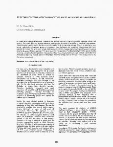
Fig. 1.

1797

Contour plot of the spectrogram of a musical pattern played by Greek traditional clarinet.

care for such deviations, we will see that, by modifying the cost function used in the Viterbi algorithm, so that to specifically account for such types of errors, the overall recognition performance can drastically improve. The philosophy on which we shall construct the HMMs follows two directions. 1) The architecture of each HMM will be developed so that to account for and incorporate some of the possible deviations within its structure. 2) Some of these deviations can be effectively treated by an appropriate modification of the cost function. It must be emphasized that this technique is of a more general scope, and other types of deviations, e.g., [5], could also be effectively integrated within the HMM architecture. After carefully studying the problem, we have concluded (also in cooperation with musicologists) that the most common deviations, frequently met in practice, belong to either of six categories. Before discussing possile deviation types in more detail, let us first present the structure of the prototypes. A. Prototypes of Musical Patterns The above discussion suggests that for a predefined set of pattern classes, against which the unknown pattern is matched, (1) can serve as the basis to define a prototype (“ideal”) pattern per class. In the case of Western classical music, each prototype could result from the direct interpretation of a printed score, ’s. In the case which would lead to specific values for the of Greek traditional music, which is also the case for eastern type traditional music in general, although printed scores are not available, it is still possible to define the values of the ’s for each prototype selected to represent each class. The classes have been shaped and categorized through everyday practice over the years by traditional instrument players.

In the sequel, assuming a total of adopt the notation

prototypes (classes), we

for each one of the known prototypes, where . As an example, one of the twelve prototypes that we studied in the , consists of five context of Greek traditional music, namely notes and, assuming a quarter-tone resolution is adopted, the resulting sequence for this prototype possesses the structure

Section VI lists all twelve prototypes that are encountered in the music corpus of our study. B. Deviations From the Prototypes Given the prototype of a class, we will now turn our attention to the possible ways that an observed pattern from the class can deviate from the respective prototype. 1) In the simplest case, only note durations should vary. In other words, any instance of a class should differ from the respective prototype only in the number of zeros ’s. Such duration variations are very separating the common in practice, due to performance variations of the instrument players, even when a printed score is followed. 2) A second type of deviation occurs when a transition between notes takes place. At a frame level, the transition is likely to span a number of consecutive frames. Although in the prototype, a note transition , is represented by a single value, i.e., a single in practice, the transition may also appear as a sequence of music intervals, the sum of which is equal

1798


Fig. 2. Quantized fundamental frequencies corresponding to the musical pattern of Fig. 1.

to the respective , of the prototype. Figs. 1 and 2 , was present a pattern of the class whose prototype, given in Section III-A. The resulting symbol sequence is . It can be seen that symbol of the prototype is broken into two successive and , whose sum is equal frequency jumps, i.e., (Fig. 2). In the general case, of a prototype to can be broken into successive frequency jumps, that are reflected in a subsequence of symbols ( ’s), in the respective feature sequence, i.e., (2) where . Note also, that (2) allows for two (or more) successive nonzero symbols, as is the case when one or more successive frames result in different pitch values. This type of deviation is an artifact of the moving window nature of most fundamental frequency tracking algorithms. It can be considered equivalent to a substitution of a music interval by a sequence of intervals of very small duration. It is worth noticing that, in certain cases, this type of substitution can also be due to improvizations of the instrument players, or even due to a performer’s error. In the context of Greek traditional music, such improvizations are encountered quite frequently. , that 3) In some cases, a subsequence of zeros, say , is replaced by forms part of a note duration, or , where and cancel out. In the more general case, subsequence is replaced by or , where and cancel out, as it is the case with octave errors. Fig. 2 demonstrates two such cases: (a) a subsequence of zeros, , corresponding to the first note of the the

, is replaced by a sequence of the form and (b) a subsequence of zeros, , , is replaced by a corresponding to the last note of . In the general sequence of the form case, such errors are due to the fundamental frequency tracking algorithm and, although they do not correspond to frequency jumps perceived by the human ear, they cause problems in the recognition algorithm. 4) A special case of deviations occurs when a subpattern of a prototype is repeated in succession a number of times, due to improvizations of the instrument players. The number of repetitions is likely to vary, depending on the context in which the specific musical pattern is performed. This is a common phenomenon in the context of Greek and Eastern type traditional music, where improvization plays a central role. 5) Missing notes can also be observed for a number of instances in a class. This suggests that certain ’s and associated zero-valued subsequences of the prototype are missing from the feature sequence of the signal to be classified. 6) As a last case, it is possible that, for certain patterns of a class, a number of music intervals are higher or lower than the respective intervals of the prototype. This phenomenon is encountered more frequently in microtonal music (quarter-tone resolution) and can be due to errors in the feature extraction stage or even due to the performance of the instrument players. prototype

C. Architecture of the Variable Duration HMMs Having given a broad categorization of the possible types of deviation from the prototypes occurring in practice, we now proceed to describe the architecture of the HMMs that model the


Fig. 3. Discrete observation, variable duration HMM that models instances of the same musical pattern, in the case of deviations of type (1).

pattern classes, and to see how the possible deviations can lead to the modified cost function. 1) A Simple Case: We start with a simple case, namely the deviations of type (1). In other words, let us first assume that only note durations are allowed to vary and that the time variation of each note can be modeled by a Gaussian probability den, where , for a sity function, total of notes. Despite its simplicity, this assumption leads immediately to the idea of using a variable-duration HMM ([25], [27]) per pattern class, provided that the states of the HMM are carefully chosen so as to reflect the general structure of the sequences given by (1). As it has already been mentioned, the time duration of each note corresponds to a subsequence of zeros in the feature sequence. Therefore, taking the prototype of a class as a starting point, the respective HMM should possess one state per sub, . Additionally, for each sequence of zeros , , a separate state is created. For notational purposes, the states corresponding to the zero valued suband the states corresequences are named Z-states, ’s are the S-states, . The reason sponding to that different zero-states are used is that this allows a different state duration model to be adopted for each state, something that is dictated by the nature of our signals. As a result, for a pattern consisting of a sequence of notes, the respective HMM consists of states (see Fig. 3). It has to be pointed out that, according to this approach, each note of the prototype corresponds to a pair of states, namely a nonzero state followed by a zero-state, with the exception, of course, of the first note (Fig. 3). If only deviations of type (1) occurred in practice, it would suffice to assume that each Z-state only emits zeros and each . In addition, is alS-state emits only the respective ways the first state. Furthermore, the state duration for each Z-state will be modeled by a Gaussian probability density . Similarly, function (pdf), namely, in order to account for deviations of type (2), a Gaussian pdf, , is also adopted for the S-states. The HMM of Fig. 3 possesses a strict architecture, i.e., it is is followed by an a left-to-right model, where each Z-state . In addiS-state , and each is definitely followed by tion, each Z-state emits only zeros with probability equal to one, , with proband each S-state emits the respective symbol, and are always the ability equal to one. Furthermore, first and last states respectively. Obviously, for this strict HMM, the only parameters that need to be reestimated, following a training procedure, are the mean values and standard deviations of the Gaussian probability density functions that model the state durations (Section V).

1799

Fig. 4. note.

Transition

Z

!S

accounts for the possibility of a missing ith

Translated in the HMM terminology, let be the resulting variable duration HMM, where is the vector of initial probabilities, is the state transition mais the symbol probability matrix ( is the trix and matrix, maximum allowed music interval). Regarding the the first element of the th row is equal to the mean value of the Gaussian function modeling the duration of the th state and the second element of the th row is the standard deviation of the respective Gaussian. For any HMM, like the one shown is always the first state suggests that in Fig. 3, the fact that and , . In addition, is upper triangular, and each element of the first diagonal of is equal to one and all other elements of have zero values. Finally, for the Z-states, each column of has only one element with value equal to 1, (and all other elements are zero valued) and similarly, for each S-state, and all other elements are zero valued. The HMM architecture described so far may serve as a starting point for dealing with the rest of the deviations described in Section III-B. 2) Missing Notes: In particular, the case of missing notes [deviations of type (5)] can be accounted for, if certain additional state transitions are permitted. Without loss of generality, we assume that no more than one successive note can be missing. Following the notation that we have so far adopted, if the th note is expected to be absent, from certain instances of a class, then a transition from to , denoted as , should also be made possible, as shown in Fig. 4. This is be, cause the th note corresponds to the pair of states th note starts at state , whereas and, similarly, the the th note ends at state . For each transition , the respective element of , namely , has a positive value. Each element of the first diagonal of has now a positive value less than one, so that the sum of each row of is equal to one. 3) Repeated Subpatterns: In the same manner, accounting for successive repetitions of a subpattern of the prototype [see deviations of type (4)], leads to permitting backward state transitions to take place. For instance, if notes are expected to form a repeating pattern, then clearly, the backmust be added (see Fig. 5). This ward transition th note ends at state , whereas the is because the th note starts at state . Matrix is no longer upper trianhas a positive value. gular, and each element 4) Music Intervals That are Higher or Lower Than the Respective Intervals of the Prototype: This situation can be dealt with if each S-state is allowed to emit music intervals that are of the prototype. For higher or lower than the respective quarter tone resolution, each S-state may also emit symbols and . This suggests that, for a column of the

1800


Fig. 5.

Transition Z

!S

accounts for the possibility of a repeated subpattern.

matrix which refers to a S-state, nonzero probabilities will and also have to be assigned to elements . These probabilities are expected to take , which is now assmaller values compared to signed a value less than one. The final values of , , and are determined by the training algorithm (see Section V). To conclude, if all patterns of a class were “corrupted” only by deviations of type (1), (4), (5), and (6), then it would suffice to adopt the aforementioned architecture for the HMMs, according to which, deviations are dealt with by changing the and matrices. 5) Deviations of Type (2) and (3)—The Need for a Modified Viterbi Algorithm: In practice, , the number of extracted notes from an unknown musical pattern, is rarely equal to the number of notes of the respective prototype, mainly due to deviations of type (2) and (3). Such is the case of the pattern shown in Fig. 1, which can be considered as an instance of the prototype

Fig. 2 shows the fundamental frequency tracking results for this pattern, after quantization has taken place, having used Tolonen’s pitch analysis model [30]. It can be seen that the extracted symbol sequence deviates from what is expected and has the structure

. If one applies these transformations to the symbol equal to becomes original feature sequence , the new sequence

which is different from , only in the number of zeros separating the positive valued symbols. In the sequel, we demonstrate that it is possible to enhance the standard variable duration HMM with a mechanism of an optimal decision making, by modifying the Viterbi algorithm ([25]–[27]), which determines, for a given feature sequence , and a trained HMM , the best-state sequence. IV. RECOGNITION PHASE In order to proceed further, certain definitions must first be be the best-state sequence, genergiven. Let ated by the Viterbi algorithm for a given observation sequence and a discrete observation variable duraas tion HMM . Let us also define the forward variable in [25], i.e., state ends at (3) stands for the probability that the model finds itself that is, in the th state after the first symbols have been emitted. It can be shown that [25], [26] (4)

If is given as input to an HMM, which was built following the procedure described so far, a zero recognition probability would occur, which is clearly undesirable. reveals that, , On the other hand, careful observation of , which is equal to , cancel out [dewhich is equal to 1 and viation of type (3)), and so do and (one more deviation , which is the respecof type (3)]. In addition, tive music interval of the prototype [deviation of type (2)]. These observations lead us to the idea that one can enhance the performance of the variable duration HMM, by inserting in the model a mechanism capable of deciding which symbol cancellations and are desired. For example, regarding sequence , if are canceled out, the subsequence can be replaced by a single subsequence of zeros, , whose length is the actual duration of the first musical note. This, in turn, suggests that if a modified version of , say, , was generated by taking into account the aforementioned symbol canwould possess a structure closer to the class protocellation, . This idea, also, applies to symbols and (which type and which sum also cancel out). Concerning symbols , it is desirable to treat subsequence as one to

(5) where is the time duration variable, is its maximum allowable value within any state, is the total number of states, is the state transition matrix, is the duration probability distribution at state , and is the symbol probability matrix. In other words, the probability of a path ending its state sequence at state depends on all possible ways to have reached state , including the possibility of remaining at state for successive time instances. We have already made the assumption that follows a Gaussian probability density function. The overall is computed from recognition probability

where a symbol sequence of length has been assumed. Equacanditions (4) and (5) suggest that there exist , for the maximization of each quandate arguments, . In order to retrieve the best state sequence, i.e., for tity


1801

backtracking purposes, the state that corresponds to the argument that maximizes (4) has to be stored in a two-dimensional . array , as Therefore

In addition, the number of symbols spent on state is stored in a two-dimensional matrix , as . Let us now focus on the deviations of type of type (2), i.e., or . As it was deviations of the type and are not real music intervals, and if previously stated, they were canceled out, the resulting subsequence would consist entirely of zeros. Therefore, for the Z-states (which have so far been assumed to only emit sequences of zeros), it is desirable to modify (4) and (5), so as to reflect the need to be able to check for subsequences that contain symbols that can be canceled out. We notice that in (4), each candidate argument refers to symbols of the observation sequence, and this is is calculated in (5). If the why the product value of is equal to zero, this indicates a possible symbol cancellation. Thus, if these successive symbols add to zero, one must take into consideration that the symbols could be the result of an error, and must be replaced by a zero that lasts for successive time instances. Of course, since one cannot be sure that this cancellation is the correct action, it is left to the optimal option process to decide, by providing the cancellation option as an extra argument in the optimization. This is quantified by considering additional arguments to augment (4), namely (6) This equation is only computed if fore, for the Z-states (4) and (5) become

. There-

(7) (8)

if

(9)

Thus, maximization is now computed over all and quantities. So, if indeed in the unknown sequence such errors occur, then error cancellation will provide a higher maximum. It is also worth noticing that if (7) is maximized by a argument, say , then the number of symbols spent at state is equal to , as is the case with the standard variable duration model. In addition, for state , state is the winning predecessor state. If, in the end, it turns out that for some states of the best-state sequence, a symbol cancellation took place, it is useful to store

this information in a separate two-dimensional matrix by setelement equal to “1” (a zero indicates ting the respective that no symbol cancellation took place). Matrices and are still used for backtracking purposes. We will now deal with deviations of type (3). In this case, refers to we must focus on the S-states. Therefore, if an S-state, then a symbol summation is desirable, if the sum is equal to the actual symbol associated with the respective S-state of the prototype. In the same rationale as before, if this holds true, the whole subsequence of symbols is treated as one symbol equal to the respective sum and again, additional arguments must be computed for , according to the following equation: (10) Therefore, for the S-states (4) and (5) become

(11)

(12)

if

(13)

Similar to the previous case, maximization is again computed over all and quantities. If (11) is maximized by a argu, then the number of symbols spent at state ment, say is equal to , as is the case with the standard variable duration model. In addition, state is the predecessor of state in the path. If a symbol summation took place, it is useful to store this information in the matrix, that was previously introduced, element equal to “1” (a zero inby setting the respective dicates that no symbol summation took place). Matrices and are still used for backtracking purposes, as it is done in the standard variable duration HMM. The need to account for possible symbol summations reveals the fact that, although in the first place, the HMM was expected to spend one frame at each S-state, it turns out that a Gaussian probability density function must also be associated with each S-state. However, upon initializing the respective mean values and standard deviations for these Gaussians, , the maximum allowable state duration, should have a smaller value for the S-states, compared to the Z-states. To conclude, the above enhancements to the Viterbi algorithm apply to the calculation of the best-state sequence and associand a ated recognition probability given a feature sequence variable duration HMM . In Section V, we will focus on the training algorithm for the HMMs and study the training algorithm in the light of the aforementioned enhancements.

1802


V. TRAINING THE HMMs For the training phase, we assume that for each class, symbol sequences are available, namely, a set of , in order to train the respective HMM . The goal of the training stage is to maximize the to adjust the model parameters . This is achieved probability by means of an iterative procedure. During each iteration, is presented to the input of each observation sequence , the the respective variable duration HMM and for each best-state sequence is calculated by means of the modified Viterbi algorithm that was introduced in Section IV. Let denote the best-state sequence associated with symbol sequence . The reestimation equations for the Viterbi algorithm stem from the cumulative processing of all best-state sequences and are based on counting frequencies of events. A key concept lies in the fact that, when symbol summations have taken place for certain states in a best path, the number of symbols spent at these states is equal to the number of symbols that were summed. Similarly, for symbol cancellations, the number of symbols spent at the associated states in a best path includes the number of symbols that were canceled. These suggest that the reestimation formulas are similar to those of a conventional variable duration HMM ([25], [26]). Therefore, the following hold. is always the first state, no reestimation of ma• If trix is necessary. However, for some pattern classes, more flexibility is required, as it is the case when the first note is likely to be missing for a number of instances of the class. To account for this phenomenon, matrix is initialized with positive values for a the number of Z-states (usually for the first two Z-states) and after each iteration step of the training stage, each is reestimated according to the equation no. of times is the first state in the best path , taking into account all s. (no. of transitions from state to state • no. of transitions from state , , taking into account all s. If then by the definition of the variable duration HMM ([25]). average number of symbols spent at state , taking • into account all occurrences of state in all ’s. deviation from of the number of symbols spent • at state , taking into account all occurrences of state in all ’s. • Concerning matrix , we must distinguish between two cases. a) In the simplest case, only zeros are emitted from a Z-state, and each S-state only emits the respective . Therefore, no reestimation of is necessary. b) However, in practice, for the patterns that we studied, we observed that, due to errors in the fundamental frequency tracking stage and due to performance errors or improvizations of the instrument players, certain music intervals can be one quarter tone higher or lower than the respective ’s of the prototype. This can be accommodated if, upon initialization, each S-state is also allowed to emit, with a small probability, symbols that are one

quarter tone higher/lower than the symbol associated with the respective S-state. As a result, each column of that corresponds to an S-state has more than one positive elements. Depending on the frequency of such cases, as an option, one can choose not to reestimate the matrix and rely on the probabilities set upon initializing the model. If, on the other hand, one chooses to reestimate the matrix as well, this can be done according to the following procedure. If state is an S-state, then it has either emitted a single — symbol or a symbol resulting from a summation of symbols (a summation is treated as one symbol equal to their sum). Therefore, the total number of symbols emitted by state is equal to the number of occurrences . Conseof state in all best-state sequences, say quently, for the S-states, the reestimation formula for the matrix is , where is an S-state, upon initializing the matrix (i.e., before the training stage begins) and is the number of times was emitted from state as a single symbol or as a result of a symbol summation. If is a Z-state, no reestimation of is necessary, be— cause the Z-states are only allowed to emit zeros, even if symbol cancellations have taken place. The aforementioned training procedure has taken into account all deviations listed in Section III-B and is general enough to account for more types of deviations, depending on the application data. As an example, consider a case where the Z-states can be also allowed to emit subsequences of the form or (i.e., the Z-states are also allowed to emit ’s or ’s that do not cancel out). Concerning the elements of the matrix that refer to the Z-states, this leads to the following variant of the reestimation formula. is the best-state sequence associated with symbol • If , we can assume that consists of a sequence total of states, i.e., . Clearly, a number of symbols have been emitted by each , say . If is a Z-state, it has either emitted zeros (even if symbol cancellations have taken place), or it has emitted zeros plus a (or ). Therefore, if is a Z-state, then denotes the total number of symbols spent at state and path . is the total number Consequently, of symbols spent at state for all best-state sequences. is the total number of zeros emitted by state , • If taking into account all best-state sequences, then . In addition, for certain occurrences of the Z-state , a or might have been emitted, i.e., certain ’s or ’s have not taken part in a symbol cancellation event. If and are the number of such occurrences for and respectively, then and . VI. APPLICATION OF THE METHOD IN THE CONTEXT OF GREEK TRADITIONAL MUSIC The proposed classification scheme, although applicable also to Western type of music, was tested in the context of Greek traditional music, since this is a more difficult classification


1803

TABLE I CLASS PROTOTYPE

task. To this end, we assembled a music corpus consisting of twelve pattern classes. We focused on monophonic patterns of Greek traditional clarinet, an instrument that closely resembles the western-type clarinet. A. Description of the Music Corpus The choice of pattern classes was suggested by musicologists on the basis of 1) their common use in practice and 2) the time elasticity exhibited by patterns of the same class. Time elasticity refers to both note duration and pattern duration as a whole, while preserving musical function [34]. All twelve types of patterns have been shaped and categorized through everyday practice over the years. The musical system of Greek traditional music and the techniques of clarinet players give the resulting sound material a radically different structure when compared with that of the Western equal-tempered intervalic system (system of musical scales) [29], [34]. Four Greek clarinet players were recorded under laboratory conditions with an ambient noise of less than 5 dB. Each player was asked to perform the same pattern a large number of times according to his improvizational skills and the resulting sound stream was manually segmented and categorized. As a result, a music corpus was assembled, consisting of 1200 monophonic patmusical patterns involving all twelve pattern classes ( terns per class). All pattern deviations listed in Section III-B can be observed in the resulting sound material. Table I presents the prototypes of the twelve classes, assuming quarter-tone resolution has been adopted. The table reveals the fact that, repeating subpatterns can be observed for certain prototypes, as is the case with classes VII, VIII, X, and XII. Although the number of repetitions of a subpattern is likely to vary among patterns of a class, Table I assumes for simplicity that, for each subpattern, the average number of such repetitions appears in the structure of the respective prototype.

B. Feature Extraction Details 1) Implementation Details of the Fundamental Frequency Tracker: For the feature generation stage, we tested a number of robust fundamental frequency tracking algorithms, including Tolonen’s multipitch analysis model [30], Brown’s narrowed autocorrelation method [31], and Brown’s pattern recognition algorithm based on the constant-Q transform [32]. After extensive experimentation, Tolonen’s method [30] was chosen as the fundamental frequency tracker of our music corpus and certain parameter tuning was decided. Specifically: 1) The length of the moving window was set equal to 50 ms (each window was multiplied by a Hamming function) and a 5-ms step was adopted between successive windows. This small step ensures that rapid changes in musical patterns are captured effectively by the pitch tracker, to the expense of increasing the length of the feature sequence. Rapid changes are observed especially in the case of pattern classes VII, VIII, XI, and XII. 2) The preprocessing stage involving a prewhitening filter was omitted. For the two channel filter bank, we used butterworth bandpass filters with frequency ranges 70–1000 Hz and 1000 Hz–10 KHz. Finally, the parameter which controls frequency domain compression was set equal to 0.7. 2) Quantization: For the quantization step, quarter-tone resolution was adopted and an alphabet of 121 discrete symbols was used, implying music intervals in the range of quarter-tones, i.e., . Our choice for quarter-tone resolution stems from the microtonal nature of the music corpus and allows for capturing quarter-tone improvizations by the instrument players. In addition, this permits the treatment of pattern classes with intervals that are odd multiples of the quarter-tone, although in the present case all music intervals of the prototypes

1804


If (14) is computed for all pairs of classes, a scatter matrix is generated (12 12 in our case). Consequently, the average class divergence, say is

TABLE II CONFUSION MATRIX

(15)

The average class divergence associated with modeling of this paper is one order of magnitude higher than the respective values obtained for the model in [29]. are even multiples of the quarter-tone (suggesting that half-tone resolution could have been adopted instead). 3) Training and Classification Results: The training set for each musical pattern consisted of 60 observation sequences, which exhibited the deviations from the prototype presented in Section III-B. A total of 480 patterns were used as the test set, uniformly distributed among pattern classes. At an average, for each variable duration HMM, the reestimation algorithm converged after (approximately) 40 iterations. Ninety-five percent of the patterns in the test set were successfully classified. Wrong classification was detected for of the patterns, whereas of the patterns generated zero recognition probability for all classes. The structural similarity of patterns belonging to classes III and IV (see also Table I) was the main reason of classification errors. The confusion matrix of Table II summarizes the distribution of recognition failures among the classes considered (only the classes for which is confusion was detected are shown). The number at cell equal to the percentage of test patterns that have been wrongly classified as type patterns instead of (the correct) type patterns. Empty cells correspond to a zero error rate. Patterns that generate a zero recognition probability for all classes, originate from classes VII and VIII. Due to the rapid changing nature of these patterns, the fundamental frequency tracker failed to capture the respective structure, thus resulting to severely distorted feature sequences. Compared with the results in [29], the classification scheme of this paper achieves comparable recognition rates. However, the HMM architecture in [29] was based on standard HMMs, where each type of deviation was modeled by a branch of states, resulting in a very complex model with large transition matrix that is hard to train. In addition, class separability was considerably inferior for the models in [29] compared with the modeling of this paper. Class separability is a very important and relates to the performance of a classifier. To this end, class divergence between a pair of classes and [28] has been used as a separability measure, as defined in (14), where stands for a are the HMMs, modfeature sequence of the test set and , eling classes , and , respectively. Equation (14) suggests that overlapping classes yield low values, whereas highly separable classes generate high values.

(14)

C. Implementation Details Related to the Enhanced Viterbi Algorithm An observation that further improves class separability is the following: In the beginning and end of certain patterns, due to low energy, or even due to the manual segmentation process, the pitch tracker is likely to produce certain errors that appear as music intervals of short duration. The average duration of this phenomenon is 0.3 s. This is shown in Fig. 6 for a pattern of class II. Despite this phenomenon, patterns are still classified correctly, because we permit the first and last state of each HMM to emit, in addition to a zero with high probability, all other symbols with a very small probability. As a result, despite correct classification, for such patterns, the recognition probability is considerably lower compared with other patterns of the class that do not possess this endpoint characteristic. In order to minimize the effects of such phenomena, a new type of state was added, both in the beginning and in the end of each HMM, which we call the end-state. Each end-state is allowed to emit any symbol with equal probability and the maximum state duration for the end states is set equal to 0.4 s. Furthermore, and may now emit only zeros, like all the other Z-states. These imply the following. 1) The total number of states is augmented by two. and , the successor to 2) If the end states are named is and is now the rightmost state of the model. is no longer the only allowable first state, therefore we 3) and . choose and may be the last state of the 4) Both music inbest state sequence, for a pattern of is the recognition probability, then tervals. If , where is the is the length of the feature seforward variable and is the first state in the best path, quence. In addition, if i.e., if the aforementioned phenomenon is also observed in the beginning of a pattern, then it makes sense to with the contribution of to the recognition divide probability. Consequently, if symbols are spent at , is the actual recognition probability. As a result, the aforementioned (annoying) phenomenon is minimized from both ends of a pattern (if it exists) resulting to higher recognition probabilities and also to enhanced class separability. It has to be noted that, the end-states may be attached to an HMM after the training stage is completed.


1805

Fig. 6. Quantized fundamental frequencies corresponding to a musical pattern of class II. The arrows point to pitch tracking artifacts at both ends of the pattern.

Fig. 7. Quantized fundamental frequencies corresponding to a musical pattern of class II. Quarter-tone resolution has been adopted.

D. A Real Case Demonstrating the Enhanced Viterbi Algorithm

tized fundamental frequencies for this pattern is shown in Fig. 7. The feature sequence corresponding to Fig. 7 is

The following is an overall example that demonstrates the efficiency of the enhanced Viterbi algorithm by means of a real experiment, where a pattern of class II (Table I) is given as input to the respective variable-duration HMM. The sequence of quan-

It can be observed that the artifact in the beginning of the feature sequence manifests itself as the sequence of symbols

1806


Fig. 8.

HMM for class II.

TABLE III BEST-STATE SEQUENCE FOR THE PATTERN OF FIG. 7

. In addition, three deviations of type (2) , and can be observed, namely, , marking the beginning of the third, fourth, and fifth note respectively. Finally, the sequence of symbols is a deviation of type (3) in the duration of the last note. Fig. 8 presents the structure of the HMM for patterns of class II. It can be seen that this HMM does not permit missing notes and repeated subpatterns. As mentioned in Section VI-B3, the HMM was trained with 60 patterns of class II. At the end of and all converged to a the training stage, states , , mean state duration of 0.25 s and deviation of 0.12 s, due to the time elasticity of the patterns of this class. Similarly, for state , the mean state duration and deviation were 1 and 0.1 s, respectively. For all the S-states of the model, the mean state duration converged to the value of 25 m and the deviation from the mean state duration to 5 ms. Table III presents the best-state sequence generated by the enhanced Viterbi algorithm. The first column of this table is the state-id, the second column shows the sequences of symbols spent at each state, the third column presents the action that was taken by the enhanced Viterbi algorithm (simple emission, summation or cancellation), and the last column demonstrates the evolution of the logarithm of the classification probability. As it was stated in Section VI-C, the symbol sequence of the artifact does not contribute to the classification probability and, therefore, the logarithm of , corresponding to the sixteen symbols comprising the artifact, is subtracted in the last column. The best-state sequence and recognition probability that were generated by the novel Viterbi algorithm verify that all deviations, which would otherwise lead

to poor classification performance, were successfully dealt with.

VII. CONCLUSION AND FUTURE WORK This paper presented a novel modified Viterbi algorithm for the calculation of recognition probabilities, generated by variable-duration HMMs. The new algorithm proved to be capable of providing enhanced classification performance of musical patterns to predefined classes. Also, a new methodology for constructing such HMMs was presented. It allows for ways to build into the structure of the HMM possible deviations in the observation sequence, due either to errors or to music players’ improvization. A case study involving patterns originating in the context of Greek traditional music was employed, although the method can be applicable to Western type of music as well. For future work, the proposed Viterbi algorithm will be used as a building block for melody spotting in raw audio recordings, that may either contain a single instrument performing in solo mode, or an ensemble of instruments, where one of the instruments has a leading role. REFERENCES [1] E. Wold et al., “Content-based search, classification and retrieval of audio,” IEEE Multimedia Mag., vol. 3, no. 3, pp. 27–36, Fall 1996. [2] J. Foote, “An overview of audio information retrieval,” Multimedia Syst., vol. 7, no. 1, pp. 2–10, 1999. [3] N. Leavitt, “Let’s hear it for audio mining,” IEEE Comput. Mag., vol. 35, no. 10, pp. 23–25, Oct. 2002. [4] M. Mongeau and D. Sankoff, “Comparison of musical sequences,” Comput. Humanities, vol. 24, pp. 161–175, 1990.


[5] E. Cambouropoulos, T. Crawford, and C. S. Iliopoulos, “Pattern processing in melodic sequences: Challenges, caveats and prospects,” Comput. Humanities, vol. 35, no. 1, pp. 9–21, 2001. [6] L. A. Smith, R. J. McNab, and I. H. Witten, “Sequence-based melodic comparison: A dynamic programming approach,” Comput. Musicol., vol. 11, pp. 101–117, 1998. [7] A. Ghias et al., “Query by humming: Musical information retrieval in an audio database,” ACM Multimedia, pp. 231–236, 1995. [8] L. Lu et al., “A new approach to query by humming in music retrieval,” in Proc. ICME, Tokyo, Japan, 2001, pp. 22–25. [9] B. Pardo and W. Birmingham, “Query by humming: How good can it get?,” in Proc. Workshop on Music Information Retrieval, Toronto, ON, Canada, 2003, pp. 107–109. [10] W. Chai and B. Vercoe, “Folk music classification using hidden Markov models,” in Proc. Int. Conf. Artificial Intelligence, Las Vegas, NV, Jun., 25–28 2001. [11] E. Cambouropoulos, “A general pitch interval representation: Theory and applications,” J. New Music Res., vol. 25, no. 3, Sep. 1996. [12] C. Raphael, “Automatic segmentation of acoustic musical signals using hidden Markov models,” IEEE Trans. Pattern Anal. Mach. Intell., vol. 21, no. 4, pp. 360–370, Apr. 1999. [13] J.-J. Aucouturier and M. Sandler, “Finding repeating patterns in acoustic musical signals :Applications for audio thumbnailing,” in Proc. AES 22nd Int. Conf. Virtual, Synthetic, Entertainment Audio, Espoo, Finland, Jun. 2002, pp. 412–421. [14] H. Shih et al., “An HMM-based approach to humming transcription,” in Proc. IEEE Int. Conf. Multimedia and Expo, ICME, vol. 1, 2002, pp. 337–340. [15] J. Pickens et al., “Polyphonic score retrieval using polyphonic audio queries: A harmonic modeling approach,” in Proc. ISMIR, Paris, France, 2002, pp. 140–149. [16] S. Shwartz et al., “Robust temporal and spectral modeling for query by melody,” in ACM SIGIR, Tampere, Finland, 2002, pp. 331–338. [17] J. Paulus and A. Klapuri, “Measuring the similarity of rhythmic patterns,” in Proc. ISMIR, 2002, pp. 150–156. [18] A. S. Durey and M. A. Clements, “Melody spotting using hidden Markov models,” in Proc. ISMIR, Bloomington, IN, Oct. 2001, pp. 109–117. [19] E. Coyle and I. Shmulevich, “A system for machine recognition of music patterns,” in Proc. ICASSP, Seattle, WA, May 1998, pp. 3597–3600. [20] J. Aucouturier and F. Pachet, “Music similarity measures: What’s the use?,” in Proc. of ISMIR, 2002, pp. 157–163. [21] R. Dannenberg and N. Hu, “Discovering musical structure in audio recordings,” in Lecture Notes in Computer Science and Artificial Intelligence. New York: Springer Verlag, 2002, vol. 2445, LNCS/LNAI, pp. 133–143. [22] D. Meredith, K. Lemström, and G. A. Wiggins, “Algorithms for discovering repeated patterns in multidimensional representations of polyphonic music,” J. New Music Research, vol. 31, no. 2, pp. 321–345, 2002. [23] D. Fragoulis et al., “On the automated recognition of seriously distorted musical recordings,” IEEE Trans. Signal Process., vol. 49, no. 4, pp. 898–908, Apr. 2001. [24] G. Evangelista, “Pitch-synchronous wavelet representations of speech and music signals,” IEEE Trans. Signal Process., vol. 41, no. 12, pp. 3313–3330, Dec. 1993. [25] L. R. Rabiner, “A tutorial on hidden Markov models and selected applications in speech recognition,” Proc. IEEE, vol. 77, no. 2, pp. 257–286, Feb. 1989. [26] J. Picone, “Continuous speech recognition using hidden Markov models,” IEEE Acoustics, Speech, Signal Process. Mag., vol. 7, no. 3, pp. 26–41, Jul. 1990. [27] L. Rabiner and B. Juang, Fundamentals of Speech Recognition. Englewood Cliffs, NJ: Prentice Hall, 1993. [28] S. Theodoridis and K. Koutroumbas, Pattern Recognition, 2nd ed. New York: Academic, 2003. [29] A. Pikrakis, S. Theodoridis, and D. Kamarotos, “Recognition of isolated musical patterns using hidden Markov models,” in Lecture Notes in Computer Science and Artificial Intelligence. New York: Springer Verlag, 2002, LNCS/LNAI 2445, pp. 133–143. [30] T. Tolonen and M. Karjalainen, “A computationally efficient multipitch analysis model,” IEEE Trans. Speech Audio Process., vol. 8, no. 6, pp. 708–716, Nov. 2000.

1807

[31] J. C. Brown and B. Zhang, “Musical frequency tracking using the methods of conventional and narrowed autocorrelation,” J. Acoust. Soc. Amer., vol. 89, no. 5, pp. 2346–2354, 1991. [32] J. C. Brown, “Musical fundamental frequency tracking using a pattern recognition method,” J. Acoust. Soc. Amer., vol. 92, no. 3, pp. 1394–1402, 1992. [33] A. Pikrakis, S. Theodoridis, and D. Kamarotos, “Recognition of isolated musical patterns using context dependent dynamic time warping,” IEEE Trans. Speech Audio Process., vol. 11, no. 3, pp. 175–183, May 2003. [34] S. Karas, Theoritikon—Methodos on Greek Traditional Music (in Greek). Athens, Greece: Association for the Popularisation of Greek Music, 1982.

Aggelos Pikrakis received the diploma in computer engineering and informatics from the University of Patras, Patras, Greece, and the Ph.D. degree in signal processing from the University of Athens, Athens, Greece. He is currently a Research Fellow at the University of Athens. His research interests are in the areas of signal processing for music with emphasis on Greek traditional music, content-based music retrieval, and intelligent agents for data mining applications.

Sergios Theodoridis (SM’03) received the honors degree in physics from the University of Athens, Athens, Greece, and the M.Sc. and Ph.D. degrees from the Department of Electronics and Electrical Engineering of Birmingham University, Birmingham, U.K. He is currently a Professor of signal processing and communications in the Department of Informatics and Telecommunications, University of Athens. His research interests lie in the areas of adaptive algorithms, channel equalization, pattern recognition, signal processing for music, and OCR systems. He has extensively published in prestigious international journals and refereed conferences. He is the coeditor of the book Adaptive System Identification and Signal Processing Algorithms (Prentice Hall, 1993) , coauthor of the book Pattern Recognition (Academic Press, 2nd ed., 2003), and of three books in Greek, two of them for the Greek Open University. Prof. Theodoridis is currently an Associate Editor for the IEEE TRANSACTIONS ON SIGNAL PROCESSING and the IEEE Signal Processing Magazine, and a member of the editorial boards of the EURASIP journals Signal Processing and Applied Signal Processing. He was the General Chairman of EUSLPCO-98, and he is the Technical Program co-Chair for ISCAS-2006. He has served as Vice Chairman of the Greek Pedagogical Institute and he was a member of the Board of Directors of COSMOTE (the Greek DCS-1800 mobile phone operating company) for four years. He is currently the President of EURASIP.

Dimitris Kamarotos studied music and computers in Athens, Greece, and continued musicology, composition, clarinet, and electronic music in Paris, France. His postgraduate research focused on the creation of tools for semiautomated music composition (IR-CAM 1984). Since 1986, he has worked as a Research Manager on many projects in collaboration with Athens Polytechnic School, University of Thessaloniki, Thessaloniki, Greece, and the Center for Contemporary Music Research. He was Research Manager of the HXE Project on creation of tools for the automated comparison of audio patterns. The same idea of automated pattern recognition extended into a monophonic musical environment was the field of research in collaboration with Prof. S. Theodoridis and Dr. A. Pikrakis. He also collaborated with B. Garton and T. Rikakis (Columbia University, NY) and P. Cook (Princeton University, Princeton, NJ) in the foundation of the computer music studio in CCMR and IPSA.