8th European Conference on Non-Destructive Testing (ECNDT 2002), Jun. 17-21, 2002, Barcelona, Spain
1
CLASSIFICATION OF POTENTIAL DEFECTS IN THE AUTOMATIC INSPECTION OF ALUMINIUM CASTINGS USING STATISTICAL PATTERN RECOGNITION Domingo Mery* and Dieter Filbert** *
**
Departamento de Ingeniería Informática Universidad de Santiago de Chile Av. Ecuador 3659 Santiago de Chile
Institut für Energie und Automatisierungstechnik Technische Universität Berlin Einsteinufer 19, D-10587 Berlin
(
[email protected] ) http://www.diinf.usach.cl/~dmery/
(
[email protected] ) http://mt.tu-berlin.de/~filbert/
Abstract In this paper we report the results obtained recently by classifying potential defects in the automated x-ray inspection of aluminium castings using statistical pattern recognition. In our classification, 71 features (e.g. area, perimeter, roundness, invariant moments, Fourier descriptors, mean grey level, several contrasts, texture features, etc.) were analysed to characterise the potential flaws. The extracted features were measured from more than 10.000 regions segmented in 56 radioscopic images (without frame averaging) of cast aluminium wheels. In addition, five statistical classifiers were tested.
1. Introduction In a digital radioscopic image of an aluminium casting there are two classes of regions (of pixels): regions that belong to regular structures of the specimen, and regions that correspond to flaws. In the computer aided inspection of castings, we aim to make the best recognition of these two classes automatically. Usually, the pattern recognition process consists of three steps [Castleman96]: The first one is called image segmentation, in which each region is found and isolated from the rest of the scene. The second step is called feature extraction. This is where the regions are measured and some significant characteristics are quantified. The third step of pattern recognition is classification. The extracted features of each region are analysed and assigned to one of the classes (regular structure or flaw). In this paper we report the results obtained recently by analysing 71 features (e.g. area, perimeter, roundness, invariant moments, Fourier descriptors, mean interior grey level, several contrasts, texture features, etc.) measured from more than 10.000 regions segmented in 56 radioscopic images of cast aluminium wheels. In order to make a compact pattern representation and a simple decision strategy, the number of features are reduced using a Sequential Forward Selection [Jain00]. In this selection, correlated features are omitted ensuring a small intraclass variation and a large interclass variation in the space of the selected features. A new developed contrast feature is presented, which separates the two classes at best.
2
8th European Conference on Non-Destructive Testing (ECNDT 2002), Jun. 17-21, 2002, Barcelona, Spain
Additionally, five statistical classifiers (linear, threshold, nearest neighbourhood, Mahalanobis and Bayes) are analysed. In the statistical approach, each segmented region is represented in terms of the m selected features and is viewed as a point in a m-dimensional space. The objective of the statistical pattern recognition is to establish decision boundaries in the feature space which separate patterns (our segmented regions) belonging to different classes (regular structure or flaw). This will be determined by the probability distributions of the patterns belonging to each class, which must be learned.
2. Segmentation of potential flaws The idea of the segmentation process is to detect regions that may correspond to real defects. The segmentation is achieved using a Laplacian-of-Gaussian (LoG) kernel and a zero crossing algorithm [Mery02b,Catleman96]. The LoG-operator involves a Gaussian lowpass filter which is a good choice for the pre-smoothing of our noisy images. The binary edge image obtained should produce at real flaws closed and connected contours which demarcate regions. In order to increase the number of closed regions, pixels with high gradient are added to the zero crossing image. An example is illustrated in Fig. 1. After the edges are detected the closed regions are segmented and considered as potential flaws.
3. Feature extraction In order to discriminate the false alarms in the segmented potential flaws a classification must be performed. The classification analyses the features of each region and classifies it in one of the following two classes: regular structure or hypothetical flaw. In this section, we will explain the features that are used in the classification. In our description, the features will be divided into two groups: geometric and grey value features. The description of the features will be made using the example of Fig. 2.
(a) radioscopic image with three flaws.
(b) edge detection.
Figure 1. Segmentation of potential flaws.
8th European Conference on Non-Destructive Testing (ECNDT 2002), Jun. 17-21, 2002, Barcelona, Spain
1 2 3 4 5 6 7 8 9 10 11
1 2 3 11
4 5 6 7 8 9 10
3
j Pixel (4,6) g[i,j]
i (a)
(b)
j
(c)
i
Figure 2. Example of a region: a) X-ray image, b) segmented region, c) 3D representation of the grey values.
3.1 Geometric features The used geometric features are: Height and width ( h and w ): These features are defined as: h = imax − imin + 1 and
w = j max − jmin + 1
(1)
where imax , j max and imin , j min correspond to the maximal and minimal values in the region that take index i and index j respectively in the image matrix. In our example h = w = 7 pixels. Area ( A ): The area is defined as the number of pixels that are in the region. In this work the edges do not belong to the region. In our example, the area corresponds to the number of grey pixels in Fig. 2b, i.e. A = 45 . Perimeter ( L ): The perimeter corresponds to the number of pixels in the boundary of the region. There is another definition of perimeter that includes the factor 2 between diagonal pixels of the boundary [Castleman96]. Although this definition is more precise, the computing time is more expensive. For this reason, we use the first definition. In this example L = 24 pixels. Roundness ( R ): This feature gives a measure of the shape of the region. The roundness is defined as R=
4 Aπ L2
(2)
The roundness R is a value between 1 and 0. R = 1 means a circle, and R = 0 corresponds to a region without area. In our example R = 0,98 . Moments: The statistical moments are defined by: m rs =
∑i
r
js
for
r, s ∈ Ν
(3)
i , j∈ℜ
where ℜ is the set of pixels of the region. In our example of Fig. 2b, the pixel (4,6) belongs to this set. The parameter r + s is called the order of the moment. There is only one zeroorder moment m00 that corresponds to the area A of the region. The coordinates of centre of gravity of the region are:
8th European Conference on Non-Destructive Testing (ECNDT 2002), Jun. 17-21, 2002, Barcelona, Spain
4
i=
m01 m00
j=
and
m10 m00
(4)
The central moments are position invariant. They are calculated using (i , j ) as origin by:
∑ (i − i )
µ rs =
r
( j − j) s
for
r, s ∈ Ν
(5)
i , j∈ℜ
With the central moments one can compute the Hu central moments [Hu62,Sonka98]. These normalised moments are invariant under magnification, translation and rotation of the region:
φ1 φ2 φ3 φ4 φ5 φ6 φ7
η20 − η02 (η20 − η02 ) 2 + 4η112 (η30 − 3η12 ) 2 + (3η21 − η03 ) 2 (η30 + η12 ) 2 + (η21 + η03 ) 2 (η30 − 3η12 )(η30 + η12 )[(η30 + η12 ) 2 − 3(η21 + η03 ) 2 ] + (3η21 − η03 )(η21 + η03 )[3(η30 + η12 ) 2 − (η21 + η03 ) 2 ] = (η20 − η02 )[(η30 + η12 ) 2 − (η21 + η03 ) 2 ] + 4η11 (η30 + η12 )(η21 + η03 ) = (3η21 − η03 )(η30 + η12 )[(η30 + η12 ) 2 − 3(η21 + η03 ) 2 ] − (η30 − 3η12 )(η21 + η03 )[3(η30 + η12 ) 2 − (η21 + η03 ) 2 ]
= = = = =
(6)
with
ηrs =
µ rs µ 00t
t=
,
r+s + 1. 2
Fourier descriptors: The coordinates of the pixels of the boundary are arranged as a complex number ik + j· j k , with j = − 1 and k = 0,..., L − 1 , where L is the perimeter of the region. The complex boundary function can be considered as a periodical signal of period L . The Discrete Fourier Transformation gives a characterisation of the shape of the region. The Fourier coefficients are defined by: L −1
Fn = ∑ (ik + j· j k )e
−j
2πkn L
for
n = 0,..., L − 1
(7)
k =0
The Fourier descriptors correspond to the coefficients Fn for n > 0 . They are invariant under rotation. The Fourier descriptors of our example in Fig. 2a are illustrated in Fig. 3. The first pixel of the periodic function is (i0 , j 0 ) = (6,10) .
3.2 Grey value features These features are computed using the grey values in the image, where x[i, j ] denotes the grey value of pixel (i, j ) . Mean grey value ( G ): The mean grey value of the region is computed as:
8th European Conference on Non-Destructive Testing (ECNDT 2002), Jun. 17-21, 2002, Barcelona, Spain
5
12
200
|Fn |
180
10
jk
160 140
8
120
ik
6
100 80
4
60 40
2
20 0
5
0
10
20
15
0
k
0
5
10
20
15
n
Figure 3. Coordinates of the boundary of region of Fig. 2 and the Fourier descriptors. x x´ Region 0
x´´ neighbourhood
neighbourhood
i
Figure 4. Profile x, first derivative x' and second derivative x'' of a region and its neighbourhood in i direction G=
1 ∑ x[i, j ] A i , j∈ℜ
(8)
where ℜ is the set of pixels of the region and A the area. A 3D representation of the grey values of the region and its neighbourhood in our example is shown in Fig. 2c. In this example G = 121,90 ( G = 0 means 100% black and G = 255 corresponds to 100% white). Mean gradient in the boundary ( C ): The average gradient around the contour line of the region gives information about the change of the grey values in the boundary of the region. It is computed as: C=
1 ∑ x' [i, j ] L i , j∈l
(9)
where x' [i, j ] means the gradient of the grey value function in pixel (i, j ) and l the set of pixels that belong to the boundary of the region. The number of pixels of this set corresponds to L , the perimeter of the region. Using a Gauss gradient operator in our example in Fig. 2, we obtain C = 35,47 .
6
8th European Conference on Non-Destructive Testing (ECNDT 2002), Jun. 17-21, 2002, Barcelona, Spain
Mean second derivative ( D ): This feature is computed as D=
1 ∑ x' ' [i, j ] A i , j∈ℜ
(10)
where x' ' [i, j ] denotes the second derivative of the grey value function in pixel (i, j ) . The Laplacian-of-Gauss (LoG) operator can be used to calculate the second derivative of the image. If D < 0 we have a region that is brighter than its neighbourhood as shown in Fig. 4. Contrast of the region: The contrast gives a measure of the difference in the grey value between the region and its neighbourhood. The smaller the grey value difference, the smaller the contrast. In this work region and neighbourhood define a zone. The zone is considered as a window of the image:
g [i, j ] = x[i + ir , j + j r ]
(11)
for i = 1,..., 2h + 1 and j = 1,..., 2 w + 1 , where h and w are the height and width as expressed in (1). The offsets ir and j r are defined as ir = i − h − 1 and j r = j − w − 1 , where ( i , j ) denotes the centre of gravity of the region as computed in (4). There are many definitions of contrast. Some of them are given in [Kamm98]:
K1 =
G − GN GN
K2 =
G − GN G + GN
K 3 = ln(G / G N )
(12)
where G and G N denote the mean grey value in the region and in the neighbourhood respectively. Other two definitions are given in [Mery01] where new contrast features are suggested. According to Fig. 5 these new features can be calculated in four steps: i) we take the profile in i direction and in j direction centred in the centre of gravity of the region ( P1 and P2 respectively); ii) we calculate the ramps R1 and R2 that are estimated as a first order function that contains the first and the last point of P1 and P2 ; iii) new profiles without background are computed as Q1 = P1 − R1 and Q2 = P2 − R2 . They are putted together as a new function Q = [Q1 , Q2 ] ; iv) The new contrast features are given by: Kσ = σ Q
K = ln(Qmax − Qmin )
and
(13)
where σ Q , Qmax and Qmin are the standard deviation, the maximal value and the minimal value of Q respectively. Fig. 5 shows the computation of function Q for the example given in Fig. 2. Moments: We can consider grey value information in the moments explained in the previous Section, if we compute the moments as: m' rs =
∑i
r
j s x[i, j ]
for
r, s ∈ Ν
(14)
i , j∈ℜ
Substituting mrs by m' rs in (6), new Hu moments φ '1 ,Lφ ' 7 that include the grey values of the region are obtained.
8th European Conference on Non-Destructive Testing (ECNDT 2002), Jun. 17-21, 2002, Barcelona, Spain
7
Texture features: These features give information about the distribution of the grey values in the image. In this work however, we restrict the computation of the texture features for a zone only defined as region and neighbourhood (see equation (11)). A simple texture feature is the local variance [Jähne97]. It is given by: 1 σ = 4hw + 2h + 2 w 2 g
2 h +1 2 w +1
∑ ∑ (g [i, j ] − g ) i =1
2
(15)
j =1
where g denotes the mean grey value in the zone. Other texture features can be computed using the co-occurrence matrix Pkl [Castleman96]. The element Pkl [i, j ] of this matrix for a zone is the number of times, divided by N T , that grey-levels i and j occur in two pixels separated by that distance and direction given by the vector (k ,l ) , where N T is the number of pixels pairs contributing to Pkl . In order to decrease the size N x × N x of the cooccurrence matrix the grey scale is often reduced from 256 to 8 grey levels.
Table 1. Extracted features Feature
Variable
Name and equation
Feature
Variable
Name and equation
1 2
h w
height (1a)
27
K
new contrast (12b)
width (1b)
28... 34
φ '1 Lφ ' 7
3
A
area
35
σ g2
4
L
perimeter
36... 39
H , I , E , Z 10
texture features k,l=10
5
R
roundness (2)
40... 43
H , I , E , Z 20
texture features k,l=20
6...12
φ1 Lφ 7
Hu moments (6)
44... 47
H , I , E , Z 30
texture features k,l=30
13...19
F1 L F7
Fourier descriptors (7)
48... 51
H , I , E , Z 01
texture features k,l=01
20
G
mean grey value (8)
52... 55
H , I , E , Z 02
texture features k,l=02
21
C
mean gradient (9)
56... 59
H , I , E , Z 03
texture features k,l=03
22
D
mean 2th derivative (10)
60... 63
H , I , E , Z 11
texture features k,l=11
23...25
K1 L K 3
contrasts 1, 2, 3 (12)
64... 67
H , I , E , Z 22
texture features k,l=22
26
Kσ
deviation contrast (12a)
68... 71
H , I , E , Z 33
texture features k,l=33
Hu moments' (6) (14) local variance (15)
(16), (17), (18), (19).
From the co-occurrence matrix several texture features can be computed. For example
8th European Conference on Non-Destructive Testing (ECNDT 2002), Jun. 17-21, 2002, Barcelona, Spain
8
180
P1
Q
P2
=Q2
=Q1
R1
R2
0 1
2
3
4
5
6
7
8
9
10
11
1
2
3
4
5
(a )
6
8
7
9
10
11
1
3
2
5
4
6
7
9
8
(b )
10
11
12
13
14
15
16
17
18
19
20
21
(c )
Figure 5. Computation of Q for contrast features: a) Profile in i direction, b) profile in j direction, c) fusion of profiles: Q= [Q1 Q2]. Nx Nx
H kl = ∑∑ Pkl [i, j ]ln(Pkl [i, j ])
entropy
(16)
i =1 j =1
Nx Nx
I kl = ∑∑ (i − j ) Pkl [i, j ]
inertia
2
(17)
i =1 j =1
Nx Nx
E kl = ∑∑ (Pkl [i, j ])
energy
2
(18)
i =1 j =1
inverse difference moment
Nx Nx
Z kl = ∑∑ i =1 j =1
Pkl [i, j ]
1 + (i − j )
(19)
2
The extracted features are summarised in Table 1.
4. Classification The classification analyses the features of each segmented region and classifies it in one of the following two classes: regular structure or hypothetical flaw. The definitive classification of the hypothetical flaws takes place in a next step called matching and tracking [Mery01,Mery02a]. In the classification we aim to discriminate the false alarms without eliminating the real flaws. Although the methodology outlined in this section is applied to only two classes, it can be used for more classes. For instance, we can subclassify the hypothetical flaws into the classes cavity, gas, inclusion, crack, and sponging.
4.1 Feature selection In the feature selection we must decide which features of the regions are relevant to the classification. The extracted features in our experiments are n = 71 as shown in Table 1. T The n features are arranged in a n -vector: w = [w1 L wn ] that can be viewed as a point in a n -dimensional space. The features are normalised as ~ = wij − w j w
σj
for
i = 1,..., N 0
and
j = 1,..., n
(20)
8th European Conference on Non-Destructive Testing (ECNDT 2002), Jun. 17-21, 2002, Barcelona, Spain
9
where wij denotes the j -th feature of the i -th feature vector, N 0 is the number of the sample, and w j and σ j are the mean and standard deviation of the j -th feature. The normalised features have zero mean and standard deviation equal to one. The key idea of the feature selection is to select a subset of m features (m < n) that leads to the smallest classification error. The selected m features are arranged in a new m T vector z = [z 1 L z m ] . The selection of the features is done using the Sequential Forward Selection [Jain00]. This method selects the best single feature and then adds one feature at a time which in combination with the selected features maximises the classification performance. Once no considerable improvement in the performance is achieved -by adding a new feature-, the iteration is stopped. By evaluating the selection performance we ensure: i) a small intraclass variation and ii) a large interclass variation in the space of the selected features. For the first condition the intraclass-covariance is used: N
C b = ∑ p k [z k − z ][z k − z ]
T
(21)
k =1
where N means the number of classes, p k denotes the a-priori probability of the k -th class, z k and z are the mean value of the k -th class and the mean value of the selected features. For the second condition the interclass-covariance is used: N
C w = ∑ pk C k
(22)
k =1
where the covariance matrix of the k -th class is given by:
[
][
1 Lk Ck = ∑ z kj − z k z kj − z k Lk − 1 j =1
]
T
(23)
with z kj the j -th selected feature vector of the k -th class, Lk is the number of samples the k -th class. The selection performance can be evaluated using the spur criterion for the selected features z :
J = spur(C −w1C b )
(24)
The larger the objective function J , the higher the selection performance.
4.2 Design of the classifier Once the proper features are selected, a classifier can be designed. In this work, the classifier assigns a feature vector z to one of the two classes: regular structure (false alarm) or hypothetical flaw, that are labelled with ‘0’ and ‘1’ respectively. In statistical pattern recognition the classification is performed using the concept of similarity: patterns that are similar are assigned to the same class [Jain00]. Although this approach is very simple, a good metric that defines the similarity must be established. With a representative sample we can make a supervised classification finding a discriminant function d (z ) that
10
8th European Conference on Non-Destructive Testing (ECNDT 2002), Jun. 17-21, 2002, Barcelona, Spain
gives information about how similar is a feature vector z to the feature vector of a class. In this work we use the following five classifiers:
Linear classifier: A linear or a quadratic combination of the selected features is used for a polynomial expansion of the discriminant function d (z ) . If d (z ) > θ then z is assigned to class ‘1’, else to class ‘0’. Using a least-square approach, the function d (z ) can be estimated from an ideal known function d * (z ) , that is obtained from the representative sample [Borner88]. Threshold classifier: The decision boundaries of class ‘1’ define a hypercube in feature space, i.e. if the m features are located between some decision thresholds ( z '1 ≤ z1 ≤ z ' '1 and ... and z ' m ≤ z m ≤ z ' ' m ) then the feature vector is assigned to class ‘1’. The thresholds are set from the representative sample [Fukunaga90]. Nearest neighbour classifier: A mean value z k of each class of the representative sample is calculated. A feature vector z is assigned to class ‘k’ if the Euclidean distance z − z k is minimal. The mean value z k can be viewed as a template [Fukunaga90].
Mahalanobis classifier: By the Mahalanobis classifier we use the same idea of the nearest neighbour classifier. However, a new distance metric called the ‘Mahalanobis distance’ is used. The Mahalanobis distance between z k and z is defined as : d k (z, z k ) =[z − z k ] C −k1 [z − z k ] T
(25)
The Mahalanobis classifier takes into account errors associated with prediction measurements, such as noise, by using the feature covariance matrix C k to scale features according to their variances [Ruske88].
Bayes classifier: The feature vector z is assigned to class ‘k’ if the probability that z belongs to this class is maximal. This conditional probability can be expressed as p(k | z ) =
p(z | k ) p k p(z )
(26)
where p (z | k ) denotes the conditional probability of observing feature vector z given class ‘k’, p(z ) means the probability that feature vector z will be observed given no knowledge about the class, and p k is the probability of occurrence of class ‘k’ [Fukunaga90, Ruske88].
4.3 Results of the classification In this section we report the results obtained by analysing the mentioned 71 features (see Table 1) measured from S = 10.609 regions segmented in 56 radioscopic images of cast aluminium wheels. The images were captured without frame averaging. In this sample there were S 0 = 10.533 regular structures (false alarms) and only S1 =76 real flaws. After a Karhunen-Loève-Transformation [Castleman96] we can see that the information is
8th European Conference on Non-Destructive Testing (ECNDT 2002), Jun. 17-21, 2002, Barcelona, Spain
11
contained in few components as shown in Fig. 6a. This means that a feature selection must be done in order to omit correlated features. The first 15 features selected by the Sequential Forward Selection are shown in Fig. 6b. We can see, that the best single feature is the feature number 27, the new developed contrast feature K (see equation (13b)). In addition, we observe that three of the best five features correspond to the texture feature energy E30 , E11 , E 22 (features 46, 62 and 66), obtained from equation (18) with (k , l ) = (3,0), (1,1) and (2,2). Furthermore, the geometric features do not provide relevant information to separate the classes. The reason is because the regions corresponding to flaws and regular structures have similar shapes. The performance of the five explained classifiers (linear, threshold, nearest neighbour, Mahalanobis and Bayes) were tested. For each classifier, m features from the 15 recommended features were selected. The effectiveness of the classification were measured in terms of ‘false positive’ or ‘false negative’ errors. False positive errors refer to the case where a segmented region is assigned to class ‘hypothetical flaw’ when it is a regular structure, and false negative errors refer to the case when an existing flaw is not detected. In ideal case both must be zero. Defining S 0 and S1 as the number of regular structures (class 0) and real flaws (class 1) that were segmented in the sample, we have -after the classification- S 0 regular structures that were classified as S 00 regular structures and S 01 hypothetical flaws: i.e. S 0 = S 00 + S 01 ; and the S1 real flaws that were classified as S10 regular structures and S11 hypothetical flaws: i.e. S1 = S10 + S11 . We see that S 01 and S10 correspond to the false positive and false negative errors respectively. This concepts are also referred in the literature as the False Acceptance Rate (FAR) and False Rejected Rate (FRR), defined as FAR = S 01 / S 0 and FRR = S10 / S1 . A classification can be tuned at a desired value of FAR. However, if we try to decrease the FAR of the system, then it would increase the FRR and vice versa. The Receiver Operation Curve (ROC) is a plot of FAR versus FRR which permits to assess the performance of the recognition system at various operating points [Jain00]. The five classifiers were manually tuned using thresholds and distance parameters [Mery01]. The results obtained for the Receiver Operation Curves are given in Fig. 7. Table 2 shows an example for each classifier, where a good performance was obtained. 1 0.
7
λj λ1
J
6 5
0.
4 3
0.
46
62
2 66 45
20
71 57 21 63
2
0. 0
27
7
24 22 19
(a) 10
20
30
j
40
50
60
70
1
(b)
0 1
2
3
4
5
6
7
8
9 10 11 12 13 14 15
best features
Figure 6. a) KLT Analysis, b) selected features using Sequential Forward Selection (see the feature numbers in Table 1).
8th European Conference on Non-Destructive Testing (ECNDT 2002), Jun. 17-21, 2002, Barcelona, Spain
12
FAR[%] 30
FAR[%] 30 linear
FAR[%] 30
FAR[%] 30 nearest neighbour
threshold
FAR[%] 30 Bayes
Mahalanobis
25
25
25
25
25
20
20
20
20
20
15
15
15
15
15
10
10
10
10
10
5
5
5
5
5
0
0
10
20
FRR[%]
30
0
0
10
20
30
FRR[%]
0
0
10
20
30
0
FRR[%]
0
10
20
0
30
0
FRR[%]
10
20
30
FRR[%]
Figure 7. ROC: False Rejected Rate (FRR) versus the False Acceptance Rate (FAR) for the evaluated classifiers. The marks ×,o,*, ∇, ∆ mean m = 1,2,3,4,5 features respectively. Since the automated inspection of castings must be as fast as possible, we aimed to use in the classification those features which computing timing is not expensive. An interesting result was obtained using only two features, feature 27 (contrast K ) and feature 20 (mean grey value G ). The classification effectiveness of the evaluated classifiers is shown in Fig. 8.
Table 2. Classification effectiveness FRR vs. FAR Classifier
Features
linear
27-24-21-20-2
threshold
27-71-20-24-7
nearest neighbour
27-21-19-46-7
Mahalanobis
27-7-62-66-19
Bayes
46-27-20
m =1
m=2
m=3
m=4
m=5
FRR
5,3%
5,3%
5,3%
5,3%
5,3%
FAR
9,8%
9,0%
7,7%
4,8%
4,1%
FRR
5,3%
5,3%
0%
0%
0%
FAR
29,5%
41,3%
32,5%
26,6%
23,5%
FRR
10,6%
13,2%
7,9%
9,2%
9,28%
FAR
7,2%
5,8%
5,3%
4,9%
4,7%
FRR
5,3%
5,3%
5,3%
5,3%
5,3%
FAR
11,6%
9,0%
7,9%
7,4%
7,0%
FRR
6,6%
3,9%
0%
-
-
FAR
26,4%
16,9%
10,0%
-
-
8th European Conference on Non-Destructive Testing (ECNDT 2002), Jun. 17-21, 2002, Barcelona, Spain
Classiffier
feature 20 (G)
feature space
FRR
13
FAR
• Linear
5,3%
9,6%
• Threshold
2,6%
21,1%
• Nearest neighbour
18,4%
7,1%
• Mahalanobis
10,5%
7,1%
5,3%
10,8%
• Bayes
real flaw regular structure
feature 27 (K)
Figure 8. Classification using two features: contrast K and mean grey value G.
5. Conclusion and Future Directions In this paper we propose the use of statistical pattern recognition to classify the segmented regions in a radioscopic image into two groups: regular structures and hypothetical flaws. The segmentation and the classification correspond to the first step of a method that detects flaws automatically from radioscopic image sequences [Mery01,Mery02a]. The second step tracks in an image sequence, the remaining hypothetical flaws classified in the first step. Using this second step the regular structures can be eliminated without discriminating the existing real flaws. In this first step we are not able to separate efficiently the real flaws from the regular structures as shown in the previous Section. The reason being is because we are working with noisy images that were not filtered with frame averaging. However, we think that the methodology outlined in this work can be used in other flaw detection methods, because they usually detect defects by doing a segmentation and a classification. It would be interesting to evaluate the features proposed in this paper by other detection techniques.
Acknowledgment The authors are grateful to Departmento de Investigaciones Científicas y Tecnológicas of the Universidad de Santiago de Chile, the German Academic Exchange Service (DAAD), and YXLON International X-Ray GmbH (Hamburg) for their support.
References [Boerner88]
H. Boerner and H. Strecker: Automated X-Ray Inspection of Aluminum Casting, IEEE Trans. Pattern Analysis and Machine Intelligence,1(1):79-91, 1988.
14
8th European Conference on Non-Destructive Testing (ECNDT 2002), Jun. 17-21, 2002, Barcelona, Spain
[Castleman96] [Fukunaga90] [Hu62] [Jähne97] [Jain00] [Ruske88] [Kamm98]
[Mery01] [Mery02a]
[Mery02b]
[Sonka98]
K.R. Castleman: Digital Image Processing, Prentice-Hall, New Jersey, 1996. K. Fukunaga: Introduction to statistical pattern recognition, Academic Press, Inc., Second Edition, San Diego, 1990. M.-K. Hu, Visual Pattern Recognition by Moment Invariants, IRE Trans. Info. Theory, IT(8):179-187, 1962. B. Jähne: Digital Image Processing, Springer, 4th edition, Berlin, Heidelberg, 1997. A.K. Jain, R.P.W. Duin and J. Mao: Statistical Pattern Recognition: A Review, IEEE Trans. Pattern Analysis and Machine Intelligence, 22(1):4-37, 2000 G. Ruske: Automatische Spracherkennung, Oldenburg Verlag, München – Wien, 1988. K.-F Kamm: Grundlagen der Röntgenabbildung. In “Moderne Bildgebung: Physik, Gerätetechnik, Bildbearbeitung und -kommunikation, Strahlenschutz, Qualitätskontrolle”, K. Ewen (Ed.), 45-62, Georg Thieme Verlag, Stuttgart, New York, 1998. D. Mery: Automated Flaw Detection in Castings from Digital Radioscopic Image Sequences, Dr. Köster Verlag, Berlin, (Ph.D. Thesis in German), 2001. D. Mery and D. Filbert: Automated Inspection of Moving Aluminium Castings. In Proceedings of the 8th European Conference on Non-Destructive Testing (ECNDT 2002), Jun. 17-21, 2002, Barcelona, Spain. D. Mery, D. Filbert and Th. Jaeger: Image Processing for Fault Detection in Aluminum Castings. In "Analytical Characterization of Aluminum and its Alloys", Editors: D.S. McKenzie and G.E. Totten, Marcel Dekker Inc., New York, 2002. M. Sonka, V. Hlavac and R. Boyle: Image Processing, Analysis, and Machine Vision, Second Edition, PWS Publishing, Pacific Grove, CA, 1998.