Studies and Improvements in Automatic Classification of Musical Sound Samples Arie A. Livshin, Geoffroy Peeters, Xavier Rodet Ircam - Centre Pompidou email:
[email protected],
[email protected],
[email protected]
Abstract In this article we shall deal with automatic classification of sound samples and ways to improve the classification results: We describe a classification process which produces high classification success percentage (over 95% for musical instruments) and compare the results of three classification algorithms: Multidimensional Gauss, KNN and LVQ. Next, we introduce several algorithms to improve the sound database self-consistency by removing outliers: LOO, IQR and MIQR. We present our efficient process for Gradual Elimination of Descriptors using Discriminant Analysis (GDE) which improves a previous descriptor selection algorithm (Peeters and Rodet 2002). It also enables us to reduce the computation complexity and space requirements of a sound classification process according to specific accuracy needs. Moreover, it allows finding the dominant separating characteristics of the sound samples in a database according to classification taxonomy. The article ends by showing that good classification results do not necessarily mean generalized recognition of the dominant sound source characteristics, but the classifier might actually be focused on the specific attributes of the classified database. By enriching the learning database with diverse samples from other databases we obtain a more general classifier. The dominant descriptors provided by GDE are then more closely related to what is supposed to be the distinctive characteristics of the sound sources.
1
Introduction
Successful automatic classification of musical sounds is useful in many applications - classification of audio files scattered on the Internet, automatic scoring of recorded music, automatic indexing of recordings, multimedia labeling and many others. A comprehensive review and bibliography of the research done in the field of automatic classification of sounds can be found in (Herrera, Peeters and Dubnov 2000).
The challenge of automatic classification of musical sounds poses many questions: Accuracy - is it possible to distinguish among virtually identical sounds coming from different instruments, for example certain sounds of Viola and Violin? Taxonomy - what should be the classes? Should sounds recorded in different environments using different instruments and playing techniques, classified in the same class? e.g. when classifying into musical instruments, should recordings of a string ensemble in a noisy environment and a pizzicato sound of a single violin recorded in an anechoic chamber considered the same class? Which instruments should be classified in the same classes when categorizing samples into instrument families? Generality - which are the common qualities of sounds of a specific class (e.g. the sounds of a classical guitar) which separate them from other classes, regardless of the sound database being used and the recording conditions? Validity of data - are the sound databases consistent? Do they contain "bad" or misclassified samples? In this article we deal with several aspects of the classification problem. We start by describing a sound classification process which yields high success percentage - over 95% when classifying samples from 18 different musical instruments according to the instrument name. We compare the results of the process when it uses different classification algorithms - K-Nearest-Neighbors, Multidimensional Gauss classifier and Learning Vector Quantization Neural Networks, to classify into several taxonomies. Next, we deal with the problem of outliers and sound database consistency - how do we find and remove "bad" or misclassified samples from the sound database? We introduce the Leave-One-Out outlier removal algorithm and compare its results with two other algorithms: Interquantile Range (IQR) and a supervised version of IQR - MIQR. In the next section we introduce the Gradual Descriptor Elimination algorithm (GDE) - our extension of the descriptor reduction technique in (Peeters and Rodet 2002). The output of this
algorithm can be used to reduce the number of descriptors used for classification to the minimum required to produce a user-selected classification success percentage, thus diminishing the computation complexity, space and memory consumption. This algorithm can also be used to provide a deeper view into the specific characteristics of a sound class which separate it from other classes in the sound database (e.g. - what characteristics of the sound of the Harp differentiate it from the sound of the Guitar?). The hypothetical goal of building an ideal classifier which could recognize all the sound variations of a musical instrument is a wholly different task than successfully classifying a specific sound database. In the last section we show that the results of evaluating a classification algorithm by randomly selecting disjoint learning set and test set out of the same database (which is a common practice) could be much different from the results when different databases are used for learning and testing. We will use 5 different sound databases, classify each one by all the rest put together and separately, then show that enriching the learning dataset by samples from different databases improves its generalization and allows it to classify new samples better.
Musical Instruments: The names of the musical instruments which produced the sounds, e.g. Violin, Oboe, etc.
2
3.2
2.1
The Test Set Sample Format
Throughout the document we will be using several sound databases containing samples of orchestral instruments. All the samples are 2 seconds long, monophonic and sampled in 44.1KHz with 16 bit resolution.
2.2
Sound Descriptors
For the task of automatic classification, 162 different sound descriptors were calculated for each sound sample (Peeters and Rodet 2002). During the article, each sample will be represented by a vector of its descriptor values.
2.3
Classification Taxonomies
Musical Instrument Families: The instrument families the sound sources belong to, e.g. Brass, Bowed Strings, etc. Pizzicato / Sustain: whether the sounds are pizzicato or sustained. As we do not use percussion instruments in this paper, we chose to classify Piano as pizzicato.
3
The Classification Process
In this section we describe a classification process which produces high success percentage and compare the results of three classification algorithms: Multidimensional Gauss, KNN and LVQ.
3.1
The Process in Brief
First a learning set and a test set are selected from the sound database, then a transformation matrix is computed by using Discriminant Analysis on the learning set. Both the learning and the test sets are multiplied by this transformation matrix. Then the test set is classified by the various classification algorithms using the learning set.
The Database
We test the classification process using an excerpt from the extensive IRCAM Studio OnLine sound database1. This excerpt, which we shall call SOL, contains 1325 sound samples categorized into 16 musical instrument categories, 4 instrument families and Pizzicato / Sustain. SOL is the same database used in (Peeters and Rodet 2002). Other databases are introduced later in the article.
3.3
Evaluation Method
In order to evaluate our classification process, a learning set of 66% of the samples is randomly selected from every class in the taxonomy. This set is used to classify the rest of the samples in the database, which we shall call the test set. Throughout the paper we shall call this evaluation method Standard Evaluation.
The sound samples in this paper are classified according to three different taxonomies, a slight expansion of the taxonomies used by (Peeters and Rodet 2002):
3.4
Figure 1. The classification taxonomies.
1
Linear Discriminant Analysis (LDA)
We diminish classification time by reducing the number of dimensions in the classified data and maximize the separation between classes by computing Linear Discriminant Analysis (McLachlan 1992) on the descriptor matrix of the learning set. We multiply both the learning set and the test set by the resultant projection matrix (Martin and Kim 1998, Peeters and Rodet 2002). http://www.ircam.fr/produits/technologies/sol/page-e.html
Later in the article we will refer to this process as Space Transformation.
3.5
The Classification Algorithms
We compare the average classification success of our samples by using the following classification algorithms: Multi-dimensional Gaussian classifier ("Gauss") - a good description of the algorithm can be found at (Sabin and Bailer-Jones 2000), Learning Vector Quantization ("LVQ") Neural Network (Kofidis, et al. 1996) and K-Nearest-Neighbors ("KNN") (Wetschereck and Dietterich 1995). In this article, we select the best K for the KNN algorithm from a range of 1 to 20 by using the LeaveOne-Out Cross Validation method on the learning set. Leave One Out (LOO) Cross validation Method (Kohavi 1995): To avoid the possible bias introduced by relying on any one particular division into test and learning sets, we split the p samples into a training set of size p-1 and a test of size 1 and average the error on the left-out pattern over the p possible ways of obtaining such a partition. This is called leave-oneout (LOO) cross-validation.
3.6
Classification Results
Table 1 shows the average success percentage over 20 Standard Evaluation experiments with each classification algorithm. Gauss K-NN LVQ Algorithm ¾ À Taxonomy Pizzicato/Sustain 99.58% 99.97% 99.93% Instrument Families 94.91% 95.24% 95.22% Instruments 94.12% 95.85% 88.57% Table 1. Classification results with different algorithms. We can see that the KNN algorithm produced the best results in all taxonomies. Usually the results of all three algorithms were quite similar, except in the Instruments taxonomy which has the highest number of classes and where LVQ produced considerably worse results than the other two algorithms. More Results. As well known, one of the problems of classification might be that a resulting classifier works well only for the specific dataset used for learning (overfitting). To show that our classification method works well with different sample databases and does not owe its success to some specific characteristics of the SOL database, we shall now use the same classification method on another database. The IOWA database consists of most of the samples provided online by the University of IOWA2, cut into single sound, mono files of 2 seconds. It contains 2440 sound samples, categorized into 12
2
http://theremin.music.uiowa.edu/MIS.html
musical Instrument categories, 5 instrument Families and Pizzicato/Sustain. The SOL and IOWA databases differ considerably - instruments present only in SOL are the Violin, Viola, Accordion, Trumpet, Harp and Guitar. Instruments present only in IOWA are Piano, Pizzicato Cello and Pizzicato Contrabass. There is also a difference in the sound levels - SOL had every instrument sampled in mf and ff, while IOWA also includes the pp level. This time we shall only classify using the KNN algorithm, which produced the best results in the previous section. The following results are the average success percentages over 20 classification experiments: Pizzicato / Sustain: 99.78%. Instrument Families: 98.86% Musical Instruments: 98.08% We can see that the classification process performs well with both the IOWA and SOL databases.
4 Improving the consistency of a sound database When a sound database is used for classification, it is important to check whether it contains outliers samples that might disturb the classification process. There are several types of outliers: Attribute Noise - these samples contain badly sampled sounds or garbled data. Class Noise - samples which are classified in the wrong group. Distance Outliers - samples which are correctly recorded and classified but differ so much from other samples in their group that they might actually mislead when used in a learning database. In this section we shall use three different algorithms for removing outliers from the SOL database and then compare the results by testing the database for self consistency using Standard Evaluation.
LOO IQR MIQR 99.88 - 99.97 99.87 - 99.97 99.90 - 99.98 (0) (20) (9) Instrument Families 95.36 - 95.79 96.58 - 97.13 95.47 - 95.92 95.93 - 96.43 (21) (20) (19) Instruments 95.50 - 96.04 96.07 - 96.56 95.40 - 95.95 95.80 - 96.37 (10) (20) (21) Table 2. The 95% confidence intervals of the average classification results when using different outlier removal algorithms. Pizzicato/Sustain
4.1
Original data 99.88 - 99.97
Algorithms for Removing Outliers
Interquantile Range (IQR) (Draper 1999): For every descriptor, let P1 be the value bigger than X% of the values of this descriptor, and let P2 be the value that is bigger than Y% of the values (X>Y). For example - X=99, Y=1. Remove the values that are larger than P1+(P1-P2)*C and the ones smaller than P2-(P1-P2)*C. C is some scalar (e.g. 1). The process is repeated until no outliers are found. A slightly different version, which we do not use here, is to calculate the mean and standard deviation (STD) of every descriptor, and then remove the samples where that descriptor has absolute values which are several times bigger than the STD. IQR is not a supervised method, meaning that it does not use the classification information about the learning database and thus cannot detect Class Noise. This method is good for detecting outliers in databases which lack classification information. Modified IQR (MIQR) - our version of IQR, influenced by (Laurikalla, Juhola and Kentala 2000): This is a supervised variant of Interquantile Range. Change 1: Perform IQR on each class separately and not on all the samples together. Change 2: When a sample containing an outlier in one of its descriptors is found, do not remove it immediately, but rather count for every sample the number of descriptors which produce outliers. At the end of the process remove the samples which have the largest number of outliers. Leave-One-Out (LOO) Outlier Removal: We propose and use the LOO Outlier Removal method, in which every sample in the database is removed in its turn from the database and classified by all the rest. Samples which were misclassified are permanently removed. The process reiterates until all samples are correctly classified.
4.2
Results
We shall apply these methods to the SOL sound database in order to improve its consistency, and then evaluate the results by using Standard
Evaluation with the KNN algorithm. In order to prove that the difference in the classification results after removing outliers is meaningful, we will compute the confidence intervals with 95% confidence level of the mean classification success percentage over 50 experiments. We present the 95% confidence intervals of the average classification success in table 2. The numbers in the brackets are the amount of samples removed by the algorithms. We can see that the differences in the results after applying the algorithms and the classification of the entire database are very small, which means that the SOL database is consistent and almost has no outliers at all - the samples are recorded well and classified into quite separate classes (this is not too surprising, as the Studio OnLine database, which is accessible on the web, is the result of a considerable effort). IQR, being unsupervised, has removed the same number of outliers for all taxonomies and did not do as well as the other two methods, sometimes even producing results worse than the results without removing outliers. LOO has outperformed the other two algorithms and produced confidence intervals in the Families and Instruments taxonomies that are non-overlapping with the confidence intervals of the classification results where no outliers were removed, proving that it has actually produced some gain3.
5 Gradual Descriptor Elimination (GDE) using Discriminant Analysis In the previous section we have been using LDA to calculate the linear combinations of the normalized descriptors (the projection matrix) which maximizes the between-class-scatter and minimizes the within-class-scatter. By examining these linear combinations, we see which descriptors are multiplied by the biggest coefficients, which means these descriptors are the most "important" ones for the classification (Peeters and Rodet 2002). 3
A good technique for heavy-testing of the algorithms is to deliberately introduce "bad samples" into a consistent database and then calculate the "noise to signal" ratio before and after applying each algorithm. This is out of the scope of this article.
Our GDE algorithm provides the dependencies between the number of descriptors and the average success of the classifications, revealing exactly which are the best n descriptors to keep for every desired n=1..N, where N is the number of all available descriptors. The algorithm repeats the following steps until no descriptors are left: 1. The classification success percentage of the database is estimated using the Leave One Out cross validation method. It is recorded along with the current descriptor list. The advantage of using LOO over Standard Evaluation here is that it does not depend on any random selection of a learning set and thus needs to be measured only once. 2. The descriptor matrix of the sound database is normalized using the MIN-MAX method (STA 2001) and a projection matrix is calculated using Discriminant Analysis. 3. The c-1 (c being the number of classes) nonzero generalized eigenvectors are selected out of the projection matrix. These eigenvectors are first converted to absolute values and then multiplied by the associated eigenvalues λ - for explanation on the eigenvalues in Discriminant Analysis, see (Peeters and Rodet 2002). The coefficients of every descriptor are summed over the vectors and the descriptor which has the smallest sum is removed.
5.2
90 80 70 60 50 40 30 20 10 0 162
120
100
80
60
40
20
0
Number of Descriptors
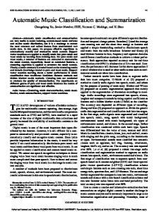
Figure 2. taxonomy
GDE
using
the
Pizzicato/Sustain
A simple example to the usefulness of the algorithm: Suppose we have a client who needs Pizzicato/Sustain classification with at least 90% average success, but also wants to save space and computation time as much as possible. Using the above results, we can offer him to decrease the number of descriptors from 162 down to 3 and still get a classification success ratio of 97.43% LOO. Families
Instruments
100
100
90 80 70 60 50 40 30 20 10
90 80 70 60 50 40 30 20 10
0 162
140
120
100
80
60
40
20
0 162
0
140
120
100
80
60
40
20
0
Number of Descriptors
Number of Descriptors
Figure 3. GDE using the Instrument Families (on the left) and the Musical Instruments taxonomies. To show that LOO results correspond closely to the results of Standard Evaluations, the following graphs depict the average results of Standard Evaluations using the same descriptors as above (produced by the GDE Algorithm), but this time performing 20 Standard Evaluations with every descriptor group - each time randomly selecting a learning set consisting of 66% of the samples4.
Results
The algorithm was applied to the SOL database. The following graphs depict the LOO classification results against the retained number of descriptors in the different taxonomies. Note that sometimes the results actually improve after removing a misleading descriptor.
140
All Instruments Leave-One-Out Success %
The Algorithm
100
All Instruments Leave-One-Out success %
5.1
Pizzicato/Sustain
All Instruments Leave-One-Out Success %
Finding out which descriptors are the dominant ones for class separation has many advantages: it enables us to save time in the future by calculating only these descriptors for new samples added to the database, save storage space, reduce classification time and memory requirements and ideally, discover which descriptors and thus which qualities really distinguish among the various sound sources. The latter will be discussed in the last section of the article.
Families
Instruments
100
100
90
90
80
80
70
70
60
60
50
50
40
40
30
30
20
20
10 0
10
160
140
120
100
80
60
40
20
0
0
160
140
120
100
80
60
40
20
0
Figure 4. GDE evaluated with Standard Evaluation. 4 This is a "Monte-Carlo showcase" which comes to show that LOO results reflect Standard results. This sort of "proofs" use the method of exemplifying a claim so many times, that it convinces that at least usually, the claim is true.
By looking at figures 3 and 4, we see that LOO is a worthy behavior quantifier for the success percentage of Standard Evaluations, although the actual averaged values depend on the size of the learning set and the number of performed classifications. Naturally, in cases where the exact percentage is very important, the LOO estimation in section 1 of the GDE algorithm could be replaced by a routine which performs the desired number of Standard Evaluation cycles and reports the average result. This change will have no effect on the selected descriptors.
6 Using Different Sound Databases for the Learning Set and the Test Set In the scientific literature, a common practice in order to evaluate the results of a sound classification algorithm is to select a learning set and a test set out of the same sound database and then try to show that the test set is classified well. We did the same in the first section of this article. As already mentioned in the introduction, an interesting question is whether the Classifiers are able to generally recognize the sounds of the sound sources (e.g. the sound of a violin) or do they only learn the specific characteristics of the database being used (underfitting the different sound possibilities of the instruments and overfitting the specific recorded samples). In this section we will show that by enriching the learning database with sound samples from other databases, we help it to generalize better the actual taxonomies it describes, thus making it more suited for classification of new sounds. We will use the following sound collections, extracted from several databases: # samples
# instruments
# families
SOL IOWA McGill
1323 2440 85
16 12 7
4 5 3
Prosonus
262
9
3
Vitus
271
8
3
Pizzicato / Sustain Both Both Only Sustain Only Sustain Only Sustain
Table 3. The sound databases used for the evaluation of mutual classification. Every sound database will be classified (using KNN) by every other database, then it will be classified using all the other databases put together (a kind of LOO which uses entire sound databases) - we shall call this method "Minus 1". In most classification cases (except the column marked "No S-T" in tables 4-6) we have performed Space Transformation using Discriminant Analysis on the learning database, and then multiplied both the learning and the test matrices by the resulting
projection matrix in order to reduce dimensionality and maximize class separation. A note about the results. We see in tables 4-6 that each sound database has a different number of instruments. In the following classifications, the instruments of the test databases which are not presented in the learning databases will be removed before classification. Due to this fact, we prevent the situation in which adding databases to the learning set improves the results simply because it adds missing instruments. On the contrary - adding an instrument to the learning set just complicates the classification Either the test database also contains this instrument; then the instrument will not be removed from the test database before classification and the classification algorithm will have to deal with an extra class (which was removed during previous classifications) - or The test database does not include the new class; this means the new class will be present only in the learning set and could only impair the results by confusing the classification algorithm.
6.1
Results5
The first column in tables 4-6 is the name of the test database. The first row shows which database was used as the learning set. Minus 1: this column shows the results of classifying the database by the rest of the databases put together. No S-T: No Space Transformation using Discriminant Analysis was performed before these classifications. Each classification had to be performed only once, as the whole test database was classified by the whole learning database. SOL IOWA Minus Minus Pizzicato classification 1 1 No S-T SOL by 98.18 98.03 97.73 IOWA by 96.68 97.05 100 McGill by 100 98.82 98.82 100 Prosonus by 99.62 98.47 100 99.62 Vitus by 98.15 94.09 97.78 100 Table 4. Results of classifying databases using other databases - the Pizzicato/Sustain taxonomy. Only SOL and IOWA have both Pizzicato and Sustain samples, therefore there is no point in using "Sustain only" databases as the learning set. 5 The ideas demonstrated in section 6 do not depend on a specific classification algorithm; KNN was used in Tables 4 - 6 only for reasons of consistency with the rest of the paper. In this section, higher classification rates can be achieved using other algorithms. Using Back-Propagation Neural Networks (Livshin and Rodet 2003) we have achieved an average Minus-1 rate of 83.17% in Instruments classification; considerably higher than the average rate of Minus-1 in Table 6 - only 60.4%.
SOL IOWA McGill Prosonus Vitus Minus 1 Minus 1 Families classification No S-T SOL by 44.60 56.42 61.67 56.50 62.13 64.02 IOWA by 75.03 74.13 66.06 70.52 86.14 78.89 McGill by 80.00 74.12 74.12 84.70 91.76 84.70 Prosonus by 77.86 58.40 74.04 55.34 84.35 77.48 Vitus by 67.90 59.78 71.95 69.74 79.70 85.98 Table 5. Results of classifying databases using other databases, the Instruments Families taxonomy. Instruments SOL IOWA McGill Prosonus Vitus Minus 1 Minus 1 classification No S-T SOL by 42.44 20.14 37.17 54.86 64.63 61.72 IOWA by 46.84 35.22 28.45 57.71 47.03 52.58 McGill by 44.70 43.53 48.23 54.12 69.41 52.82 Prosonus by 26.33 46.18 26.58 51.40 51.91 48.47 Vitus by 48.34 42.07 30.12 47.97 69.00 68.63 Table 6. Results of classifying databases using other databases, the Musical Instruments taxonomy. The tables show us that the results of classifying a sound database by several other databases are better than classifying it by any one of them separately. As already stated, the improvement does not come from addition of missing instruments to the learned dataset. These results show that enriching a learned dataset with samples from other databases (presumably recorded in different conditions by different performers using different instruments) help it to generalize better. We can also see that in the majority of the "Minus 1" classifications (the "Minus 1" column), computing LDA using the learned databases and multiplying the descriptors of both the test and learning sets by the resulting projection matrix, improves the classification results over classification results without Space Transformation (the "Minus 1 No S-T" column). This fact is not trivial. Several tests have been done where a single database was used as a learning set and another one as the test set without performing Space Transformation and in all these cases the authors noticed that the classification results were actually better without using Space Transformation. As LDA finds the descriptors which best separate the classes in the learned database, the fact that using Space Transformation improved the results when computed on several joined databases but worsened them when performed on a single one, shows that the Space Transformation selects more general descriptors when applied to the joined sets, descriptors which better represent the diverse sounds of a class. This is clearly not just the result of increasing the number of sound samples in the learning set - the IOWA database, for example, contains more samples of every instrument class than all the other databases put together but it is far from being the best learning set, as the tables show.
This difference in the LDA transformation matrix can be exemplified clearly in the following result: The authors have merged all the databases together (a total of 4381 samples) and performed a GDE using the Pizzicato/Sustain taxonomy. The last descriptor which survived (with a high classification ratio of 97% LOO) was the "effective duration" - this is "a measure of the time the signal is perceptually meaningful" (Peeters 2002), which seems to be a natural descriptor for the job. When the same process was performed using only the SOL database, the last descriptor left was the "spectral centroid", which for all opinions is not a good measure for distinguishing between Pizzicato and Sustained sounds, but probably did that in SOL due to some specific characteristics of that database. The results tend to show that one of these databases by itself covers only a small portion of the possible sounds of a class, but merging several databases helps to generalize and cover larger portions of the different sound variations belonging to a class. Finally, as intended, the tables show clearly that evaluating a classification algorithm by selecting a learning set and a test set out of the same sound database does not necessarily reflect its generalization ability - the IOWA database for example, classified its test groups in the Instruments taxonomy with an average success of 98.08% (see first section of the article), while table 6 shows that it classified the samples of SOL (of the instruments presented in both SOL and IOWA), with only 42.44% success average. An interesting future project could be to compile a very big and diverse sound database, add many new descriptors and use GDE to find the descriptors which "really" encompass the differences between the sounds of different musical instruments.
7
Conclusions
In this article we dealt with automatic classification of sound samples and presented several methods and algorithms to improve classification results: We started by showing that high classification results could be achieved with the described classification process. We compared the results of using three classification algorithms in the process: Multidimensional Gauss, KNN and LVQ. Out of these algorithms, KNN produced the best results. Then we presented several algorithms to improve the sound database self-consistency by removing outliers: LOO, IQR and MIQR. We performed them on the SOL sound database and achieved best results from the LOO algorithm. The Gradual Elimination of Descriptors using Discriminant Analysis (GDE) algorithm was presented. We showed that our algorithm allows to reduce the computation complexity and the space requirements of a sound classification process according to specific accuracy needs and to find the dominant separating characteristics of the sound samples in the database into given classes. The article ends by showing that evaluating a classification algorithm by selecting a learning set and a test set out of the same database does not necessarily reflect the algorithm generalization performance and that enriching the learning database with diverse samples from other databases improves its generalization power and could help to find more general descriptors for the class taxonomies by using the GDE algorithm. A lot of work is still to be done in order to get nearer the answers to the fundamental questions of sound classification: Is it possible to distinguish among virtually identical sounds coming from different instruments? What should be the classes in the classification taxonomies? Which are the common qualities of sounds of a specific class of musical instruments? Which sound samples could be counted as "valid"?
References Draper, N. 1999. "Statistics 201 lectures". Online statistics lectures by the Statistics Department of the Wisconsin Madison University. URL: www.stat.wisc.edu/~jyan/st201/pdf/dis10.pdf Herrera, P., Peeters, G., Dubnov, S. 2000. "Automatic Classification of Musical Instrument Sounds." submitted to the Journal of New Musical Research. URL: http://www.diku.dk/forskning/musinf/mosart/ midterm/T2/Herrera_timbre.pdf Kofidis, E., Theodoridis, S., Kotropoulos, C., Pitas, I. 1996. "Nonlinear adaptive filters for speckle suppression in ultrasonic images", Signal Processing, 52(3):357-372. URL: citeseer.nj.nec.com/kofidis96nonlinear.html Kohavi, R. 1995. "A Study of Cross-Validation and Bootstrap for Accuracy Estimation and Model Selection." IJCAI 1137-1145. Laurikalla, J. , Juhola, M., Kentala, E. 2000. "Informal identification of outliers in medical data." 5th International Workshop on Intelligent Data Analysis in Medicine and Pharmacology (IDAMAP-2000). URL: citeseer.nj.nec.com/327617.html Livshin, A., Rodet, X. 2003. "The Importance of Cross Database Evaluation in Musical Instrument Sound Classification: a critical approach." ISMIR 2003. Martin, K. D., Y. E. Kim. 1998. "Musical instrument identification: A pattern-recognition approach." Paper read at the 136 th meeting of the Acoustical Society of America. URL: citeseer.nj.nec.com/martin98musical.html McLachlan, G. J. 1992. Book title: "Discriminant Analysis and Statistical Pattern Recognition." New York, NY: Wiley Interscience. Peeters, G. 2002. "WP2.1 Preliminary Audio Descriptors." Project CUIDADO - Audio Feature Extraction: 14. Peeters, G., Rodet, X. 2002. "Automatically selecting signal descriptors for Sound Classification." ICMC 2002. URL: www.ircam.fr/equipes/analyse-synthese/peeters/ ARTICLES/ Peeters_2002_ICMC_SoundClassification.pdf Sabin, T. J., Bailer-Jones, C.A.L. 2000. "Accelerated learning using Gaussian process models to predict static recrystalisation in an Al-Mg alloy. Modelling and Simulation in Materials Science and Engineering, 8(5):687-706. URL: www.mpiahd.mpg.de/homes/calj/gpcryst.pdf STA. 2001. "STA 6938 Range and Distribution Normalization." Online Data-Mining lectures by the Department of Statistics at the University of Central Florida (UCF). URL: dms.stat.ucf.edu/sta6938notes/Lecture/Lecture2/ STA6938_Lecture2.pdf Wettschereck, D., Dietterich, T. G. 1995. "An Experimental Comparison of the Nearest-Neighbor and NearestHyperrectangle Algorithms." Machine Learning 19(1):5-27. URL: citeseer.nj.nec.com/wettschereck95experimental .html