Classification of Pre-Filtered Multichannel Remote Sensing Images

4 Classification of Pre-Filtered Multichannel Remote Sensing Images Vladimir Lukin1, Nikolay Ponomarenko1, Dmitriy Fevralev1, Benoit Vozel2, Kacem Chehdi2 and Andriy Kurekin3 National Aerospace University 2University of Rennes 1 3Plymouth Marine Laboratory 1Ukraine 2France 3UK

1

1. Introduction Multichannel remote sensing (RS) has gained popularity and has been successfully applied for solving numerous practical tasks as forestry, agriculture, hydrology, meteorology, ecology, urban area and pollution control, etc. (Chang, 2007). Using the term “multichannel”, we mean a wide set of imaging approaches and RS systems (complexes) including multifrequency and dual/multi polarization radar (Oliver & Quegan, 2004), multi- and hyperspectral optical and infrared sensors. While for such radars the number of formed images is a few, the number of channels (components or sub-bands) in images can be tens, hundreds and even more than one thousand for optical/infrared imagers. TerraSAR-X is a good example of modern multichannel radar system; AVIRIS, HYDICE, HYPERION and others can serve as examples of modern hyperspectral imagers, both airborne and spaceborne (Landgrebe, 2002; Schowengerdt, 2007). An idea behind increasing the number of channels is clear and simple: it is possible to expect that more useful information can be extracted from more data or this information is more reliable and accurate. However, the tendency to increasing the channels’ (sub-band) number has also its “black” side. One has to register, to process, to transmit and to store more data. Even visualization of the obtained multichannel images for their displaying at tristimuli monitors becomes problematic (Zhang et al., 2008). Huge size of the obtained data leads to difficulties at any standard stage of multichannel image processing involving calibration, georeferencing, compression if used (Zabala et al., 2006). But, probably, the most essential problems arise in image pre-filtering and classification. The complexity of these tasks deals with the following: a.

Noise characteristics in multichannel image components can be considerably different in the sense of noise type (additive, multiplicative, signal-dependent, mixed), statistics (probability density function (PDF), variance), spatial correlation (Kulemin et al., 2004; Barducci et al., 2005, Uss et al., 2011, Aiazzi et al., 2006);

www.intechopen.com

76 b.

c.

d.

e.

f.

g.

h.

i.

Remote Sensing – Advanced Techniques and Platforms

These characteristics can be a priori unknown or known only partly, signal-to-noise ratio can considerably vary from one to another component image (Kerekes & Baum, 2003) and even from one to another data cube of multichannel data obtained for different imaging missions; Although there are numerous books and papers devoted to image filter design and performance analysis (Plataniotis &Venetsanopoulos, 2000; Elad, 2010), they mainly deal with grayscale and color image processing; there are certain similarities between multichannel image filtering and color image denoising but the former case is sufficiently more complicated; Recently, several papers describing possible approaches to multichannel image filtering have appeared (De Backer et al., 2008; Amato et al., 2009; Benedetto et al., 2010; Renard et al., 2006; Chen & Qian, 2011; Demir et al., 2011, Pizurica & Philips, 2006; Renard et al., 2008); a positive feature of some of these papers is that they study efficiency of denoising together with classification accuracy; this seems to be a correct approach since classification (in wide sense) is the final goal of multichannel RS data exploitation and filtering is only a pre-requisite for better classification; there are two main drawbacks of these papers: noise is either simulated and additive white Gaussian noise (AWGN) is usually considered as a model, or aforementioned peculiarities of noise in real-life images are not taken into account; Though efficiency of filtering and classification are to be studied together, there is no well established correlation between quantitative criteria commonly used in filtering (and lossy compression) as mean square error (MSE), peak signal-to-noise ratio (PSNR) and some others and criteria of classification accuracy as probability of correct classification (PCC), misclassification matrix, anomaly detection probability and others (Christophe et al., 2005); One problem in studying classification accuracy is availability of numerous classifiers currently applied to multichannel images as neural network (NN) ones (Plaza et al., 2008), Support Vector Machines (SVM) and their modifications (Demir et al., 2011), different statistical and clustering tools (Jeon & Landgrebe, 1999), Spectral Angle Mapper (SAM) (Renard et al., 2008), etc.; It is quite difficult to establish what classifier is the best with application to multichannel RS data because classifier performance depends upon many factors as methodology of learning, parameters (as number of layers and neurons in them for NN), number of classes and features’ separability, etc.; it seems that many researchers are simply exploiting one or two classifiers that are either available as ready computer tools or for which the users have certain experience; Dimensionality reduction, especially for hyperspectral data, is often used to simplify classification, to accelerate learning, to avoid dealing with spectral bands for which signal-to-noise ratios (SNRs) are quite low (Chen & Qian, 2011) due to atmospheric effects; to exploit only data from those sub-bands that are the most informative for solving a given particular task (Popov et al.., 2011); however, it is not clear how to perform dimensionality reduction in an optimal manner and how filtering influences dimensionality reduction; Test multichannel images for which it could be possible to analyze efficiency of filtering and accuracy of classification are absent; because of this, people either add noise of quite high level to real-life data (that seem practically noise free) artificially or characterize efficiency of denoising by the “final result”, i.e. by increasing the PCC (Chen & Qian, 2011).

www.intechopen.com

Classification of Pre-Filtered Multichannel Remote Sensing Images

77

It follows from the aforesaid that it is impossible to take into account all factors mentioned above. Thus, it seems reasonable to concentrate on considering several particular aspects. Therefore, within this Chapter we concentrate on analyzing multichannel data information component and noise characteristics first. To our opinion, this is needed for better understanding of what are peculiarities of requirements to filtering and what approaches to denoising can be applied. All these questions are thoroughly discussed in Section 2 with taking into account recent advances in theory and practice of image filtering. Besides, we briefly consider some aspects of classifier training in Section 3. Section 4 deals with analysis of classification results for three-channel data created on basis of Landsat images with artificially added noise. Throughout the Chapter, we present examples from real-life RS images of different origin to provide generality of analysis and conclusions. One can expect that more efficient filtering leads to better classification. This expectation is, in general, correct. However, considering image filtering, one should always keep in mind that alongside with noise removal (which is a positive effect) any filter produces distortions and artefacts (negative effects) that influence RS data classification as well. Because of this, filtering, to be reasonable for applying, has to provide more positive effects than negative ones from the viewpoint of solving a final task, RS data classification in the considered case.

2. Approaches to multichannel image filtering 2.1 Information content and noise characteristics Speaking very simply, benefits of multichannel remote sensing compared to single-channel mode are due to the following reasons. First, availability of multichannel (especially hyperspectral) data allows solving many particular tasks since while for one particular task one subset of sub-band data is “optimal”, another subset is “optimal” for solving another task. Thus, multichannel remote sensing is multi-purpose allowing different users to be satisfied with employing data collected one time for a given territory. Second, useful information is often extracted by exploiting certain similarity of information content in component images and practical independence of noise in these components. Thus, efficient SNR increases due to forming and processing more sub-band images. Really, correlation of information content in multichannel RS data is usually high. Let us give one example. Consider hyperspectral data provided by AVIRIS airborne system (available at http://aviris.jpl.nasa.gov/aviris) that can be represented as I (i , j ,  ) where i  1,..., I im , j  1,..., J im denote image size and  is wavelength, k , k  1,...K defines wavelength for a k-th subband (the total number of sub-bands for AVIRIS images is 224). Let us analyze cross-correlation factors determined for neighbouring k-th and k+1-th sub-band images as R k k  1  (  ( I (i , j , k )  I mean (k ))( I (i , j , k  1 )  I mean (k  1 ))) /( I im J im k k  1 ) I im J im

i 1 j 1

I mean (k )   I (i , j , k ) /( I im J im ) I im J im

i 1 j 1

www.intechopen.com

(1)

78


 k2   ( I (i , j , k )  I mean ( k ))2 /( I im J im  1) I im J im

i 1 j 1

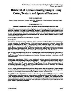
The obtained plot for AVIRIS data is presented in Fig. 1. It is seen that for most neighbour sub-bands the values of R k k  1 are close to unity confirming high correlation (very similar content) of these images. There are such k for which R k k  1 considerably differs from unity. In particular, this happens for several first sub-bands, several last sub-bands, sub-bands with k about 110 and 160. The main reason for this is the presence of noise.

1.2

Rkk+1

0.9 0.6 0.3 0 0

50

100

150

200

k

Fig. 1. The plot R k k  1 , k  1,..., 223 for AVIRIS image Moffett Field

To prove this, let us present data from the papers (Ponomarenko et al., 2006) and (Lukin et al., 2010b). Based on blind estimates of additive noise standard deviations in sub-band 2 images  ad k , robust modified estimates PSNRmod have been obtained for all channels (modifications have been introduced for reducing the influence of hot pixel values): 2 PSNRmod ( k )  10 log 10 (( I 99% ( k )  I 1% ( k ))2 /  ad k

(2)

where I q% ( k ) defines q-th percent quintile of image values in k-th sub-band image.

The plot is presented in Fig. 2. Comparing the plots in Figures 1 and 2, it can be concluded that rather small R k k  1 are observed for such subintervals of k for which PSNRmod ( k ) are also quite small. Thus, there is strict relation between these parameters. There is also relation between PSNRmod ( k ) and SNR for sub-band images analyzed in Ref. (Curran & Dungan, 1989). In this sense, one important peculiarity of multichannel (especially, hyperspectral) data is to be stressed. Dynamic range of the data in sub-band images characterized by I max ( k )  I min ( k ) (maximal and minimal values for a given k-th subband) varies a lot. Note that to avoid problems with hot pixels and outliers in data, it is also possible to characterize dynamic range by I 99% ( k )  I 1% ( k ) exploited in (2). The plot of Drob ( k )  I 99% ( k )  I 1% ( k ) is presented in Fig. 3. It follows from its analysis that a general tendency is decreasing of Drob ( k ) when k (and wavelength) increases with having sharp jumps down for sub-bands where atmospheric absorption and other physical effects take place. Though both PSNRmod ( k ) and SNR can characterize noise influence (intensity) in images, we prefer to analyze PSNRmod ( k ) and PSNR below as parameters more commonly used in practice of filter efficiency analysis. Strictly saying, PSNRmod ( k ) differs

www.intechopen.com

79


PSNRmod, dB

60 50 40 30 20 10 0 0

50

100

150

200

k

Fig. 2. PSNRmod ( k ) for the same image as in Fig. 1

Drob

6000 5000 4000 3000 2000 1000 0 0

50

100

150

200

k

Fig. 3. Robustly estimated dynamic range Drob ( k ) from traditional PSNR, but for images without outliers this difference is not large and the tendencies observed for PSNR take place for PSNRmod ( k ) as well. Noise characteristics in multichannel image channels can be rather different as well. The situation when noise type is different happens very seldom (this is possible if, e.g., optical and synthetic aperture radar (SAR) data are fused (Gungor & Shan, 2006) where additive noise model is typical for optical data and multiplicative noise is natural for radar ones). The same type of noise present in all component images is the case met much more often. However, noise type can be not simple and noise characteristics (e.g., variance) can change in rather wide limits. Let us give one example. The estimated standard deviation (STD) of additive noise for all sub-band images is presented in Fig. 4. As it is seen, the estimates vary a lot. Even though these are estimates with a limited accuracy, the observed variations clearly demonstrate that noise statistics is not constant. A more thorough analysis (Uss et al., 2011) shows that noise is not purely additive but signal dependent even for data provided by such old hyperspectral sensors as AVIRIS. Sufficient variations of signal dependent noise parameters from one band to another are observed. Recent studies (Barducci et al., 2005, Alparone et al., 2006) demonstrate a clear tendency for signal-dependent noise component to become prevailing (over additive one) for new generation hyperspectral sensors. This means that special attention should be paid to this tendency in filter design and efficiency analysis with application to multichannel data denoising and classification. Although the methods of multichannel image denoising designed on basis of the additive noise model with identical variance in all component

www.intechopen.com

80


50 STD

40 30 20 10 0 0

50

100

150

200

k

Fig. 4. Estimated STD of noise for components of the same AVIRIS image images can provide a certain degree of noise removal, they are surely not optimal for the considered task. Consider one more example. Figure 5 presents two components of dual-polarisation (HH and VV) 512x512 pixel fragment SAR image of Indonesia formed by TerraSAR-X spaceborne system (http://www.infoterra.de/tsx/freedata/start.php). Amplitude images are formed from complex-valued data offered at this site. As it is seen, the HH and VV images are similar to each other although both are corrupted by fully developed speckle and there are some differences in intensity of backscattering for specific small sized objects placed on water surface (left part of images, dark pixels). The value of cross-correlation factor (1) is equal to 0.63, i.e. it is quite small. Both images have been separately denoised by the DCTbased filter adapted to multiplicative nature of noise (with the same characteristics for both images) and spatial correlation of speckle (Ponomarenko et al., 2008a). The filtered images are represented in Fig. 6 where it is seen that speckle has been effectively suppressed. Filtering has considerably increased inter-channel correlation, it is equal to 0.85 for denoised images. This indirectly confirms that low values of inter-channel correlation factor in original RS data can be due to noise.

HH

VV

Fig. 5. The 512x512 pixel fragment SAR images of Indonesia for two polarizations

www.intechopen.com

81


HH

VV

Fig. 6. The SAR images after denoising The given example for dual polarization SAR data is also typical in the sense that noise in component images can be not additive (speckle is pure multiplicative) and not Gaussian (it has Rayleigh distribution for the considered amplitude single look SAR images). For the presented example of HH and VV polarization images statistical and spatial correlation characteristics of speckle are practically identical in both component images, but it is not always the case for multichannel radar images. The presented results clearly demonstrate that noise in multichannel RS images can be signal-dependent where its variance (and sometimes even PDF) depends upon information signal (image). Noise statistics can also vary from one sub-band image to another. These peculiarities have to be taken into account in multichannel image simulation, filter and classifier design and performance analysis. 2.2 Component-wise and vector filtering

If one deals with 3D data as multichannel RS images, an idea comes immediately that filtering can be carried out either component-wise or in a vector (3D) manner. This was understood more than 20 years ago when researchers and engineers ran into necessity to process colour RGB images (Astola et al.,1990). Whilst for colour images there are actually only these two ways, for multichannel images there is also a compromise variant of processing not entire 3D volume of data but also certain groups (sets) of channels (subbands) (Uss et al., 2011). As analogue of this situation, we can refer to filtering of video where a set of subsequent frames can be used for denoising (Dabov et al., 2007). There is also possibility to apply denoising only to some but not all component images. In this sense, it is worth mentioning the paper (Philips et al., 2009). It is demonstrated there that prefiltering of some sub-band images can make them useful for improving hyperspectral data classification carried out using reduced sets of the most informative channels. However, the proposed solution to apply the median filter with scanning windows of different size component-wise is, to our opinion, not the best choice.

www.intechopen.com

82


Thus, there are quite many opportunities and each way has its own advantages and drawbacks. Keeping in mind the peculiarities of image and noise discussed above, let us start from the simplest case of component-wise filtering. It is clear that more efficient filtering leads, in general, to better classification (although strict relationships between conventional quantitative criteria characterizing filtering efficiency and classifier performance are not established yet). Therefore, let us revisit recent achievements and advances in theory and practice of grayscale image filtering and analyze in what degree they can be useful for hyperspectral image denoising. Recall that the case of additive white Gaussian noise (AWGN) present in images has been studied most often. Recently, the theoretical limits of denoising efficiency in terms of output mean square error (MSE) within non-local filtering approach have been obtained (Chatterjee & Milanfar, 2010). The authors have presented results for a wide variety of test images and noise variance values. Moreover, the authors have provided software that allows calculating potential (minimal reachable) output MSE for a given noise-free grayscale image for a given standard deviation of AWGN. Later, in the paper (Chatterjee & Milanfar, 2011), it has been shown how potential output MSE can be accurately predicted for a noisy image at hand. This allows drawing important conclusions as follows. First, potential reduction of output MSE compared to variance of AWGN in original image depends upon image complexity and noise intensity. Reduction is large if an image is quite simple and noise variance is large, i.e. if input SNR (and PSNR) of an image to be filtered is low. For textural images and high input SNR, potential output MSE can be by only 1.2...1.5 times smaller than AWGN variance (see also data in the papers (Lukin at al., 2011, Ponomarenko et al., 2011, Fevralev et al., 2011)). This means that filtering becomes practically inefficient in the sense that positive effect of noise removal is almost “compensated” by negative effect of distortion introducing inherent for any denoising method in less or larger degree. With application to hyperspectral data filtering, this leads to the aforementioned idea that not all component images are to be filtered. The preliminary conclusion then is that sub-band images with rather high SNR are to be kept untouched whilst other ones can be denoised. A question is then what can be (automatic) rules for deciding what sub-band images to denoise and what to remain unfiltered? Unfortunately, such rules and automatic procedures are not proposed and tested yet. As preliminary considerations, we can state only that if input PSNR is larger than 35 dB, then it is hard to provide PSNR improvement due to filtering by more than 2...3 dB. Moreover, for input PSNR>35 dB, AWGN in original images is almost not seen (it can be observed only in homogeneous image regions with rather small mean intensity). Because of this, denoised and original component images might seem almost identical (Fevralev et al., 2011). Then it comes a question is it worth carrying out denoising for such component images with rather large input PSNR in the sense of filtering positive impact on classification accuracy. We will turn back to this question later in Section 4. The second important conclusion that comes from the analysis in (Chatterjee & Milanfar, 2010) is that the best performance for grayscale image filtering is currently provided by the methods that belong to the non-local denoising group (Elad, 2010; Foi et al., 2007; Kervrann & Boulanger, 2008). The best orthogonal transform based methods are comparable to nonlocal ones in efficiency, especially if processed images are not too simple (Lukin et al., 2011a). Let us see how efficient these methods can be with application to component-wise processing of multichannel RS data.

www.intechopen.com

83


Although noise is mostly signal-dependent in component images of hyperspectral data, there are certain sub-bands where dynamic range is quite small and additive noise component is dominant or comparable to signal-dependent one (Uss et al., 2011; Lukin et al., 2011b). One such image (sub-band 221 of the AVIRIS data set Cuprite) is presented in Fig. 7,a. Noise is clearly seen in this image and the estimated variance of additive noise component is about 30. The output image for the BM3D filter (Foi et al., 2007) which is currently the best among non-local denoisers is given in Fig. 7,b. Noise is suppressed and all details and edges are preserved well.

(a)

(b)

Fig. 7. Original 221 sub-band AVIRIS image Cuprite (a) and the output of BM3D filter (b) However, applying the non-local filters becomes problematic if noise does not fit the (dominant) AWGN model considered above. There are several problems and few known ways out. The first problem is that the non-local denoising methods are mostly designed for removal of AWGN. Recall that these methods are based on searching for similar patches in a given image. The search becomes much more complicated if noise is not additive and, especially, if noise is spatially correlated. One way out is to apply a properly selected homomorphic variance-stabilizing transform to convert a signal dependent noise to pure additive and then to use non-local filtering (Mäkitalo et al., 2010). This is possible for certain types of signal-dependent noise (Deledalle et al., 2011, see also www.cs.tut.fi/~foi/optvst). Thus, the considered processing procedure becomes applicable under condition that the noise in an image is of known type, its characteristics are known or properly (accurately) pre-estimated and there exists the corresponding pair of homomorphic transforms. Examples of signal dependent noise types for which such transforms exist are pure multiplicative noise (direct transform is of logarithmic type), Poisson noise (Anscombe transform), Poisson and pure additive noise (generalized Poisson transform) and other ones.

www.intechopen.com

84


Let us demonstrate applicability of the three-stage filtering procedure (direct homomorphic transform – non-local denoising – inverse homomorphic transform) for noise removal in SAR images corrupted by pure multiplicative noise (speckle). The output of this procedure exploited for processing the single-look SAR image in Fig. 5 (HH) is represented in Fig. 8,a. Details and edges are preserved well and speckle is sufficiently suppressed.

(a )

(b)

Fig. 8. The HH SAR image after denoising by the three-stage procedure (a) and vector DCTbased filtering (b) The second problem is that similar patch search becomes problematic for spatially correlated noise. For correlated noise, similarity of patches can be due to similarity of noise realizations but not due to similarity of information content. Then, noise reduction ability of non-local denoising methods decreases and artefacts can appear. The problem of searching similar blocks (8x8 pixel patches) has been considered (Ponomarenko et al., 2010). But the proposed method has been applied to blind estimation of noise spatial spectrum in DCT domain, not to image filtering within non-local framework. The obtained estimates of the DCT spatial spectrum have been then used to improve performance of the DCT based filter (Ponomarenko2008). Note that adaptation to spatial spectrum of noise in image filtering leads to sufficient improvement of output image quality according to both conventional criteria and visual quality metrics (Lukin et al, 2008). Finally, the third problem deals with accurate estimation of signal-dependent noise statistical characteristics (Zabrodina et al., 2011). Even assuming a proper variance stabilizing transform exists as, e.g., generalized Anscombe transform (Murtag et al, 1995) for mixed Poisson-like and additive noise, parameters of transform are to be adjusted to mixed noise statistics. Then, if statistical characteristics of mixed noise are estimated not accurately, variance stabilization is not perfect and this leads to reduction of filtering efficiency. Note that blind estimation of mixed noise parameters is not able nowadays to provide quite accurate estimation of parameters for all images and all possible sets of mixed noise parameters (Zabrodina et al., 2011). Besides, non-local filtering methods are usually not fast enough since search for similar patches requires intensive computations.

www.intechopen.com


85

As an alternative solution to three-stage procedures that employ non-local filtering, it is possible to advice using locally adaptive DCT-based filtering (Ponomarenko et al., 2011). Under condition of a priori known or accurately pre-estimated dependence of signal 2  f ( I tr ) , it is easy to adapt local thresholds for dependent noise variance on local mean  sd hard thresholding of DCT coefficients in each nm-th block as  T (n , m)   f ( I (n , m))

(3)

 where I (n , m) is the estimate of the local mean for this block,  is the parameter (for hard

thresholding,   2.6 is recommended). If noise is spatially correlated and its normalized spatial spectrum Wnorm ( k , l ) is known in advance or accurately pre-estimated, the threshold becomes also frequency-dependent  T (n , m , k , l )   Wnorm ( k , l ) f ( I (n , m))

(4)

where k and l are frequency indices in DCT domain. One more option is to apply the modified sigma filter (Lukin et al., 2011b) where the neighbourhood for a current ij-th pixel is formed as I min (i , j )  I ( i , j )   sig f ( I (i , j )), I max (i , j )  I ( i , j )   sig f ( I (i , j )) ,

(5)

where  sig is the parameter commonly set equal to 2 (Lee, 1980) and averaging of all image values for ij-th scanning window position that belong to the interval defined by (5) is carried out. This algorithm is very simple but not as efficient as the DCT-based filtering in the same conditions (Tsymbal et al., 2005). Moreover, the sigma filter can be in no way adapted to spatially correlated noise. 2  f ( I tr ) and Wnorm ( k , l ) , it is possible to use an Finally, if there is no information on  sd adaptive DCT-based filter version designed for removing non-stationary noise (Lukin et al., 2010a). However, for efficient filtering, it is worth exploiting all information on noise characteristics that is either available or can be retrieved from a given image.

Let us come now to considering possible approaches to vector filtering of multichannel RS data. Again, let us start from theory and recent achievements. First of all, it has been recently shown theoretically that potential output MSE for vector (3D) processing is considerably better (smaller) than for component-wise filtering of color RGB images (Uss et al., 2011b), by 1.6…2.2 times. This is due to exploiting inherent inter-channel correlation of signal components. Then, if a larger number of channel data are processed together and interchannel correlation factor is larger than for RGB color images (where it is about 0.8), one can expect even better efficiency of 3D filtering. Similar effects but concerning practical output MSEs have been demonstrated for 3D DCT based filter (Ponomarenko et al., 2008b) and vector modified sigma filter (Kurekin et al., 1999; Lukin et al., 2006; Zelensky et al., 2002) applied to color and multichannel RS images. It is shown in these papers that vector processing provides sufficient benefit in filtering efficiency (up to 2 dB) for the cases of three-channel image processing with similar noise

www.intechopen.com

86


intensities in component images. This, in turn, improves classification of multichannel RS data (Lukin et al., 2006, Zelensky et al., 2002). However, there are specific effects that might happen if 3D filtering is applied without careful taking into account noise characteristics in component images (and the corresponding pre-processing). For the vector sigma filter, the 3D neighborhood can be formed according to (5) for any a priori known dependences f(.) that can be individual for each component image. This is one advantage of this filter that, in fact, requires no preprocessing operations as, e.g., homomorphic transformations. Another advantage is that if noise is of different intensity in component images processed together, then the vector sigma filter considerably improves the quality of the component image(s) with the smallest SNR. A drawback is that filtering for other components is not so efficient. The aforementioned property can be useful for hyperspectral data for which it seems possible to enhance component images with low SNR by proper selection of other component images (with high SNR) to be processed jointly (in the vector manner). However, this idea needs solid verification in future. For the 3D DCT-based filtering, two practical situations have been considered. The first one is AWGN with equal variances in all components (Fevralev et al., 2011). Channel decorrelation and processing in fully overlapping 8x8 blocks is applied. This approach provides 1…2 dB improvement compared to component-wise DCT-based processing of color images according to output PSNR and the visual quality metric PSNR-HVS-M (Ponomarenko et al., 2007). The second situation is different types of noise and/or different variances of noise in component images to be processed together. Then noise type has to be converted to additive by the corresponding variance stabilizing transforms and images are to be normalized (stretched) to have equal variances. After this, the 3D DCT based filter is to be applied. Otherwise, e.g., if noise variances are not the same, oversmoothing can be observed for component images with smaller variance values whilst undersmoothing can take place for components with larger variances. To illustrate performance of this method, we have applied it to dual-polarization SAR image composed of images presented in Fig. 5. Identical logarithmic transforms have been used first separately for each component to get two images corrupted by pure additive noise with equal variance values. Then, the 3D DCT based filtering with setting the frequency dependent thresholds as T ( k , l )   ad c Wnorm ( k , l ) has been used where  ad c denotes additive noise standard

deviation after direct homomorpic transform. Finally, identical inverse homomorphic transforms have been performed for each component image. The obtained filtered HH component image is presented in Fig. 8,b. Speckle is suppressed even better than in the image in Fig 8,a and edge/detail preservation is good as well. Note that vector filtering of multichannel images can be useful not only for more efficient denoising, but also for decreasing residual errors of image co-registration (Kurekin1997). Its application results in less misclassifications in the neighborhoods of sharp edges.

As it is seen, the DCT-based filtering methods use the parameter  that, in general, can be varied. Analysis of the influence of this parameter on filtering efficiency for the threechannel LandSat image visualized in RGB in Fig. 9 has been carried out in (Fevralev et al., 2010). Similar analysis, but for standard grayscale images, has been performed in (Ponomarenko et al., 2011). It has been established that an optimal value of  that provides

www.intechopen.com

87


maximal efficiency of denoising according to a given quantitative criteria depends upon a filtered image, noise intensity (variance for AWGN case), thresholding type, and a metric used. In particular, for hard thresholding which is the most popular and rather efficient, optimal  is usually slightly larger than 2.6 if an image is quite simple, noise is intensive PSNR ). For complex images and small and output PSNR or MSE are used as criteria (  opt

PSNR variance of noise (input PSNR>32..34 dB),  opt is usually slightly smaller than 2.6.

Interestingly, if the visual quality metric PSNR-HVS-M (Ponomarenko et al., 2007) is employed as criterion of filtering efficiency, the corresponding optimal value is PSNR  HVS  M PSNR  opt  0.85 opt for all considered images and noise intensities. This means that if one wishes to provide better visual quality of filtered image, edge/detail/texture preservation is to be paid main attention (better preservation is provided if  is smaller).

(a)

(b)

Fig. 9. Noise free (a) and noisy (b) test images, additive noise variance is equal to 100

3. Classifiers and their training In this Section, we would like to avoid a thorough discussion on possible classification approaches with application to multichannel RS images. An interested reader is addressed to (Berge & Solberg, 2004), (Melgani & Bruzzone, 2004), (Ainsworth et al., 2007), etc. General observations of modern tendencies for hyperspectral images are the following. Although there are quite many different classifiers (see Introduction), neural network, support vector machine and SAM are, probably, the most popular ones. One reason for using NN and SVM classifiers is their ability to better cope with non-gaussianity of features. Dimensionality reduction (there are numerous methods) is usually carried out without loss in classification accuracy but with making the classification task simpler. Classifier performance depends upon many factors as number of classes, their separability in feature space, classifier type and parameters, a methodology of training used and a training sample size, etc. If training is done in supervised manner (which is more popular for classification application), training data set should contain, at least, hundreds of feature

www.intechopen.com

88


vectors and classification is then carried out for other pixels (in fact, voxels or feature vectors obtained for them). Validation is usually performed for thousands of voxels. Pixel-by-pixel classification is usually performed, being quite complex even in this case, although some advanced techniques exploit also texture features (Rellier et al., 2004). There is also an opportunity to post-process preliminary classification data in order to partly remove misclassifications (Yli-Harja & Shmulevich, 1999). The situation in classification of multichannel radar imagery is another due to considerably smaller number of channels (Ferro-Famil & Pottier, 2001, Alberga et al., 2008). There is no problem with dimensionality reduction. Instead, the problem is with establishing and exploiting sets of the most informative and noise-immune features derived from the obtained images. One reason is that there are many different representations of polarimetric information where features can be not independent, being retrieved from the same original data. Another reason is intensive speckle inherent for radar imagery where SARs able to provide appropriate resolution are mostly used nowadays. To sufficiently narrow an area of our study, we have restricted ourselves by considering the three-channel Landsat image (Fig. 9a) composed of visible band images that relate to central wavelengths 0.66 μm, 0.56 μm, and 0.49 μm associated with R, G, and B components of the obtained “color” image, respectively. Only the AWGN case has been analyzed where noise with predetermined variance was artificially added to each component independently. Radial basis function (RBF) NN and SVM classifiers have been applied. According to the recommendations given above, training has been done for several fragments for each class shown by the corresponding colors in Fig. 10b. The numbers of training samples was 1617, 1369, 375, 191 and 722 for the classes “Soil”, “Grass”, “Water”, “Urban” (Roads and Buildings), and “Bushes”, respectively. Classification has been applied to all image pixels although validation has been performed only for pixels that belong to areas marked by five colors in Fig. 10a.

(a) Image classes:

-grass,

(b) -water,

-roads and buildings,

-bushes,

Fig. 10. Ground truth map (a) and fragments used for classifier training (b)

www.intechopen.com

-soil


89

Pixel-by-pixel classification has been used without exploiting any textural features since these features can be influenced by noise and filtering. The training dataset has been formed from noise-free samples of the original test image represented in Fig. 9,a, to alleviate these impairments degrading the training results and to make simpler the analysis of image classification accuracy in the presence of noise and distortions introduced by denoising. Thus, in fact, for every image pixel the feature vector has been formed as





x q  xqR , xqG , xqB , i.e. composed of brightness values of Landsat image components

associated with R, G, and B. Details concerning training the considered classifiers can be found in (Fevralev et al., 2010). Here we would like to mention only the following. We have used the RBF NN with one hidden layer of nonlinear elements with a Gaussian activation function (Bose & Liang, 1996) and an output layer with linear elements. The element number in the output layer equals to the number of classes (five) where every element is associated with the particular class of the sensed terrain. The classifier presumes making a hard decision that is performed by selecting the element of the output layer having the maximum output value. The RBF NN unknown parameters have been obtained by the cascade-correlation algorithm that starts with one hidden unit and iteratively adds new hidden units to reduce (minimize) the total residual error. The error function has exploited weights to provide equal contributions from every image class for different numbers of class learning samples. The considered SVM classifier employs nonlinear kernel functions in order to transform a feature vector into a new feature vector in a higher dimension space where linear classification is performed (Schölkopf et al., 1999). The SVM training has been based on quadratic programming, which guarantees reaching a global minimum of the classifier error function (Cristianini & Shawe-Taylor, 2000). For the considered classification task, we have applied a Radial Basis kernel function of the same form as the activation function of the RBF NN hidden layer units. To solve multi-class problem using the SVM classifier we have applied one-against-one classification strategy. It divides the multi-class problem into S(S-1)/2 separate binary classification tasks for all possible pair combinations of S classes. A majority voting rule has been then applied at the final stage to find the resulting class. The overall probability of correct classification reached for noise-free image is 0.906 for the RBF NN and 0.915 for the SVM classifiers, respectively. The reasons of the observed misclassifications are that the considered classes are not separable as we exploited only three simple features (intensities in channel images). The largest misclassification probabilities have been observed for the classes “Soil” and “Urban”, “Soil” and “Bushes”. This is not surprising since these classes are quite heterogeneous and have similar “colors” in the composed three-channel image (see Fig. 9,a).

4. Filtering and classification results and examples Concerning Landsat data classification, let us start with considering overall probabilities of correct classification Pcc. The obtained results are presented in Table 1 for three values of AWGN variance, namely, 100, 49, and 16 (note that only two values, 100 and 49, have been analyzed in the earlier paper (Fevralev et al., 2010). The case of noise variance equal to 16 is added to study the situation when input PSNR=39 dB, i.e. noise intensity is such that noise

www.intechopen.com

90


Image

σ2



Pcc for SVM Pcc for RBF NN

Noisy

16

-

0.890

0.887

Filtered (component-wise, HT)

16

2.5

0.909

0.905

Filtered (3D, HT)

16

2.5

0.919

0.906

Noisy

49

-

0.813

0.838


49

2.5

0.889

0.903


49

2.1

0.880

0.898

Filtered (component-wise, CT)

49

3.9

0.888

0.903


49

3.3

0.879

0.896

Filtered (3D, HT)

49

2.6

0.917

0.911

Noisy

100

-

0.729

0.766


100

2.5

0.881

0.902


100

2.1

0.867

0.892


100

3.9

0.879

0.902


100

3.3

0.865

0.890

Filtered (3D, HT)

100

2.6

0.918

0.914

Table 1. Classification results for original and filtered images is practically not seen in original image (Fevralev et al., 2011). Alongside with hard thresholding (HT), we have analyzed a combined thresholding (CT) D(n , m , k , l ), if D(n , m , k , l )   ( n , m , k , l ) Dct (n , m , k , l )   3 2 2  D (n , m , k , l ) /   (n , m , k , l ) otherwise

where

 2 (n , m , k , l )  f ( I (n , m)Wnorm ( k , l ) . Note that for CT

aforementioned property

PSNR  HVS  M  opt



PSNR 0.85 opt

PSNR  opt  3.9

(6) and the

is also valid.

As it follows from analysis of data in Table 1, any considered method of pre-filtering noisy images has positive effect on classification irrespectively to a classifier used. As it could be expected, the largest positive effect associated with considerable increase of Pcc is observed if noise is intensive (see data for σ2=100 compared to „Noisy“). If noise variance is small (σ2=16), there is still improvement of image quality after filtering. Output PSNR becomes 42.4 dB after component-wise denoising and 43.0 after 3D DCT-based filtering. This improvement in terms of PSNR leads to increase of Pcc although it is not large. Probability of correct classification has sufficiently increased for classes 1 (Soil), 2 (Grass), and 5 (Bushes). Note that for filtered image Pcc is practically the same as for classification of noise-free data. This shows that if PSNR for classified image is over 42…43 dB, the (residual) noise practically does not effect classification. Both considered algorithms of thresholding produce approximately the same results for the same noise variance, classifier and component-wise filtering (compare, e.g., the cases

www.intechopen.com


91

  2.5 for HT and   3.9 for CT, σ2=100 and 49). Because of this, we have analyzed only hard thresholding for σ2=16.

PSNR  HVS  M ) The use of smaller   2.1 for HT and   3.3 for CT (that correspond to  opt PSNR . To our opinion, this results in slight reduction of Pcc compared to the case of setting  opt

can be explained by better noise suppression efficiency provided for the DCT-based filtering with larger  which is expedient for, at least, two classes met in the studied Landsat image (namely, for „homogeneous“ classes „Water“ and „Grass“ that occupy about half of pixels in validation set, see Fig. 10b). Data analysis also allows concluding that more efficient filtering provided by the 3D filtering compared to component-wise processing leads to sufficient increase in Pcc especially for intensive noise case and SVM classifier. This shows that if filtering is more efficient in terms of conventional metrics, then, most probably, it is more expedient in terms of classification. All these conclusions are consistent for both classifiers. Although the results are slightly better for the RBF NN if noise is intensive, Pcc values are almost the same for non-intensive noise. We have also analyzed the influence of filtering efficiency on classification accuracy for particular classes. Only hard thresholding has been considered (the results for combined thresholding are given in (Fevralev et al., 2010) and they are quite close to the data for hard thresholding). Three filtering approaches have been used: component-wise denoising with PSNR PSNR  HVS  M  2.1 (denoted as Filtered 2.1), component-wise filtering with  opt  opt (denoted as Filtered 2.5), and 3D (vector) processing (Filtered 3D). For the first class “Soil”, a clear tendency is observed: more efficient the filtering, larger the probability of correct classification Pcorr1. The same holds for “homogeneous” classes “Grass” (analyze Pcorr2) and “Water” (see data for Pcorr3), the attained probabilities for these classes are high and approach unity for filtered images. The dependences for the class “Bushes” (see Pcorr5) are similar to the dependences for the class “Soil”. Pcorr5 increases if more efficient filtering is applied but not essentially. Quite many misclassifications remain due to “heterogeneity” of the classes “Soil” and “Bushes” (see discussion above). Finally, specific results are observed for the class “Urban” (see data for Pcorr4). The pixels that belong to this class are not classified well in noisy images, especially by the SVM classifier. Filtering, especially 3D processing that possesses the best edge/detail preservation, slightly improves the values of Pcorr4. There is practically no difference in data for the cases Filtered 2.1 and Filtered 2.5. Thus, we can conclude that a filter ability to preserve edges and details is of prime importance for such “heterogeneous” classes. It can be also expected that the use of texture features for such classes can improve probability of their correct classification. Note that, for other classes, image pre-filtering also indirectly incorporates spatial information to classification by taking into account neighbouring pixel values at denoising stage to “correct” a given pixel value. Let us now present examples of classification. Fig. 11,a, and 11,b illustrate classification results for noisy images (σ2=100) for both classifiers. There are quite many pixel-wise misclassifications due to influence of noise, especially for the SVM classifier. Even the water surface is classified with misclassifications. In turn, Figures 11,c and 11,d present

www.intechopen.com

92


Image

σ2

Classifier

Pcorr1

Pcorr2

Pcorr3

Pcorr4

Pcorr5

Noisy

49

RBF NN

0.717

0.909

0.987

0.718

0.805

Noisy

49

SVM

0.612

0.939

0.930

0.650

0.785

Filtered 2.1

49

RBF NN

0.814

0.991

0.987

0.715

0.830

Filtered 2.1

49

SVM

0.770

0.996

0.971

0.655

0.812

Filtered2.5

49

RBF NN

0.827

0.994

0.987

0.714

0.833

Filtered 2.5

49

SVM

0.803

0.998

0.974

0.657

0.818

Filtered 3D

49

RBF NN

0.839

0.997

0.987

0.720

0.860

Filtered 3D

49

SVM

0.882

0.998

0.986

0.682

0.862

Noisy

100

RBF NN

0.649

0.790

0.984

0.718

0.776

Noisy

100

SVM

0.530

0.826

0.834

0.634

0.745

Filtered 2.1

100

RBF NN

0.811

0.983

0.986

0.718

0.819

Filtered 2.1

100

SVM

0.728

0.994

0.966

0.653

0.797

Filtered2.5

100

RBF NN

0.834

0.991

0.985

0.717

0.830

Filtered 2.5

100

SVM

0.776

0.998

0.969

0.658

0.805

Filtered 3D

100

RBF NN

0.853

0.996

0.984

0.719

0.862

Filtered 3D

100

SVM

0.888

0.998

0.985

0.687

0.858

Table 2. Classification results for particular classes of original and filtered images classification results for the three-channel image processed by the 3D DCT-based filter. It is clearly seen that quite many misclassifications have been corrected and the objects of certain classes have become compact. Comparison of the classification results in Figures 11,c and 11,d to the data in Figures 11,a and 11,b clearly demonstrate expedience of using RS image pre-filtering before classification if noise is intensive. Let us give one more example for multichannel radar imaging. Fig. 12,a shows a threechannel radar image (in monochrome representation composed of HH Ka-band, VV Kaband, and HH X-band SLAR images. The result of its component-wise processing by the modified sigma filter is presented in Fig. 12,b. Noise is suppressed but the edges are smeared due to residual errors of image co-registration and low contrasts of edges. Considerably better edge/detail preservation is provided by the vector filter (Kurekin et al., 1997) that, in fact, sharpens edges if their misalignment in component images is detected (see Fig. 12,c). Finally, the result of bare soil areas detection (pixels are shown by white) by trained RBF NN applied to filtered data is depicted in Fig. 12,d. Since we had topology map for this region, probability of correct detection has been calculated and it was over 0.93. Classification results from original co-registered images were considerably less accurate.

www.intechopen.com

93


(a)

(b)

(c)

(d)

Fig. 11. Classification maps for noisy image classified by RBF NN (a) and SVM (b) and the image pre-processed by the 3D DCT filter classified by RBF NN (c) and SVM (d)

www.intechopen.com

94


(a)

(c)

(b)

(d)

Fig. 12. Original three-channel radar image in monochrome representation (a), output for component-wise processing (b), output for vector filtering (c), classification map (d)

5. Conclusions It is demonstrated that in most modern applications of multichannel RS noise characteristics deviate from conventional assumption to be additive and i.i.d. Thus, filtering techniques are to be adapted to more sophisticated real-life models. This especially relates to multichannel radar imaging for which it is possible to gain considerably higher efficiency of denoising by taking into account spatial correlation of noise and sufficient correlation of information in component images. New approaches that take into account aforementioned properties are proposed and tested for real life data. It is also shown that filtering is expedient for RS images contaminated by considerably less intensive noise than in radar imaging. Even if noise is practically not seen (noticeable by visual inspection) in original images, its removal by efficient filters can lead to increase of data classification accuracy.

www.intechopen.com


95

6. References Abramov, S., Zabrodina, V., Lukin, V., Vozel, B., Chehdi, K., & Astola, J. (2011). Methods for Blind Estimation of the Variance of Mixed Noise and Their Performance Analysis, In: Numerical Analysis – Theory and Applications, Jan Awrejcewicz (Ed.), InTech, ISBN 978-953-307-389-7, Retrieved from Aiazzi, B., Alparone, L., Barducci, A., Baronti, S., Marcoinni, P., Pippi, I., & Selva, M. (2006). Noise modelling and estimation of hyperspectral data from airborne imaging spectrometers. Annals of Geophysics, Vol. 49, No. 1, February 2006 Ainsworth, T., Lee, J.-S., & Chang, L.W. (2007). Classification Comparisons between DualPol and Quad-Pol SAR Imagery, Proceedings of IGARSS, pp. 164-167 Alberga, V., Satalino, G., & Staykova, D. (2008). Comparison of Polarimetric SAR Observables in Terms of Classification Performance. International Journal of Remote Sensing, Vol. 29, Issue 14, (July 2008), pp. 4129-4150 Amato, U., Cavalli, R.M., Palombo, A., Pignatti, S., & Santini, F. (2009). Experimental approach to the selection of the components in the minimum noise fraction, IEEE Transactions on Geoscience and Remote Sensing, Vol. 47, No 1, pp. 153-160 Astola, J., Haavisto, P. & Neuvo, Y. (1990) Vector Median Filters, Proc. IEEE, 1990, Vol. 78, pp. 678-689 Barducci, A., Guzzi, D., Marcoionni, P., & Pippi, I. (2005). CHRIS-Proba performance evaluation: signal-to-noise ratio, instrument efficiency and data quality from acquisitions over San Rossore (Italy) test site, Proceedings of the 3-rd ESA CHRIS/Proba Workshop, Italy, March 2005 Benedetto, J.J., Czaja, W., Ehler, M., Flake, C., & Hirn, M. (2010). Wavelet packets for multiand hyperspectral imagery, Proceedings of SPIE Conference on Wavelet Applications in Industrial Processing XIII, SPIE Vol. 7535 Berge, A. & Solberg, A. (2004). A Comparison of Methods for Improving Classification of Hyperspectral Data, Proceedings of IGARSS, Vol. 2, pp. 945-948 Bose, N.K. & Liang, P. (1996). Neural network fundamentals with graphs, algorithms and applications, McGraw Hill Chatterjee, P. & Milanfar, P. (2010). Is Denoising Dead? IEEE Transactions on Image Processing, Vol. 19, No 4, (April 2010), pp. 895-911 Chatterjee, P. & Milanfar, P. (2011). Practical Bounds on Image Denoising: From Estimation to Information. IEEE Transactions on Image Processing, , Vol. 20, No 5, (2011), pp. 221-1233 Chein-I Chang (Ed.) (2007). Hyperspectral Data Exploitation: Theory and Applications, WileyInterscience Chen, G. & Qian, S. (2011). Denoising of Hyperspectral Imagery Using Principal Component Analysis and Wavelet Shrinkage. IEEE Transactions on Geoscience and Remote Sensing, Vol. 49, pp. 973-980 Christophe, E., Leger, D., & Mailhes, C. (2005). Quality criteria benchmark for hyperspectral imagery. IEEE Transactions on Geoscience and Remote Sensing, No. 43(9), pp. 21032114. Cristianini, N. & Shawe-Taylor, J. (2000). An Introduction to Support Vector Machines and Other Kernel-based Learning Methods, Cambridge University Press

www.intechopen.com

96


Curran, P.J. & Dungan, J., L. (1989). Estimation of signal-to-noise: a new procedure applied to AVIRIS data. IEEE Transactions on Geoscience and Remote Sensing, Vol. 27, pp. 20 – 628. Dabov, K., Foi,A., & Egiazarian, K. (2007). Video Denoising by Sparse 3D-Transform Domain Collaborative Filtering, Proceedings of EUSIPCO, 2007 De Backer, S., Pizurica,A., Huysmans, B., Philips, W., & Scheunders, P. (2008). Denoising of multicomponent images using wavelet least squares estimators. Image and Vision Computing, Vol. 26, No 7, pp. 1038-1051 Deledalle, C.-A., Tupin, F., & Denis, L. (2011). Patch Similarity under Non Gaussian Noise, Proceedings of ICIP, 2011 Demir, B., Erturk, S., & Gullu, K. (2011). Hyperspectral Image Classification Using Denoising of Intrinsic Mode Functions. IEEE Geoscience and Remote Sensing Letters, Vol. 8, No 2, pp. 220-224. Elad, M. (2010). Sparse and Redundant Representations. From Theory to Applications in Signal and Image Processing, Springer Science+Business Media, LLC Ferro-Famil, L. & Pottier, E. (2001). Multi-frequency polarimetric SAR data classification, Annals Of Telecommunications, Vol. 56, No 9-10, pp. 510-522 Fevralev, D., Lukin, V., Ponomarenko, N., Vozel, B., Chehdi, K., Kurekin, A., & Shark, L. (2010). Classification of filtered multichannel images, Proceedings of SPIE/EUROPTO on Satellite Remote Sensing, Toulouse, France, September 2010 Fevralev, D., Ponomarenko, N., Lukin, V., Abramov, S., Egiazarian, K., & Astola, J. (2011). Efficiency analysis of color image filtering. EURASIP Journal on Advances in Signal Processing, 2011:41 Foi, A., Dabov, K., Katkovnik, V., & Egiazarian, K. (2007). Image denoising by sparse 3-D transform-domain collaborative filtering. IEEE Transactions on Image Processing, Vol. 6, No 8, (2007), pp. 2080-2095 Gungor, O. & Shan, J. (2006). An optimal fusion approach for optical and SAR images, Proceedings of ISPRS Commission VII Mid-term Symposium „Remote Sensing: from Pixels to Processes“, Netherlands, May 2006, pp. 111-116 Jeon, B. & Landgrebe, D.A. (1999). Partially supervised classiﬁcation using weighted unsupervised clustering. IEEE Transactions on Geoscience and Remote Sensing, Vol. 37, No 2, pp. 1073–1079 Kerekes, J.P. & Baum, J.E. (2003). Hyperspectral Imaging System Modeling. Lincoln Laboratory Journal, Vol. 14, No 1, pp. 117-130 Kervrann, C. & Boulanger, J. (2008). Local adaptivity to variable smoothness for exemplarbased image regularization and representation. International Journal of Computer Vision, Vol. 79, No 1, (2008), pp. 45-69 Kulemin, G.P., Zelensky, A.A., & Astola, J.T. (2004). Methods and Algorithms for Preprocessing and Classification of Multichannel Radar Remote Sensing Images, TICSP Series, No. 28, ISBN 952-15-1293-8, Finland, TTY Monistamo Kurekin, A.A., Lukin, V.V., Zelensky, A.A., Ponomarenko, N.N., Astola, J.T., & Saarinen, K.P. (1997). Adaptive Nonlinear Vector Filtering of Multichannel Radar Images, Proceedings of SPIE Conference on Multispectral Imaging for Terrestrial Applications II, San Diego, CA, USA, SPIE Vol. 3119, pp. 25-36 Kurekin, A.A., Lukin, V.V., Zelensky, A.A., Koivisto, P.T., Astola, J.T., & Saarinen, K.P. (1999). Comparison of component and vector filter performance with application to multichannel and color image processing, Proceedings of the IEEE-EURASIP Workshop on Nonlinear Signal and Image Processing, Antalya, Turkey, June 1999, No. 1, pp. 38-42

www.intechopen.com


97

Landgrebe, D. (2002). Hyperspectral image data analysis as a high dimensional signal problem. IEEE Signal Processing Magazine, No. 19, pp. 17-28 Lee, J.-S. (1983). Digital Image Smoothing and the Sigma Filter. Comp. Vis. Graph. Image Process., No. 24, (1983), pp. 255-269 Lukin, V., Tsymbal, O., Vozel, B., & Chehdi, K. (2006). Processing multichannel radar images by modified vector sigma filter for edge detection enhancement, Proceedings of ICASSP, Vol II, pp 833-836 Lukin, V., Fevralev, D., Ponomarenko, N., Abramov, S., Pogrebnyak, O., Egiazarian, K., & Astola, J. (2010a). Discrete cosine transform-based local adaptive filtering of images corrupted by nonstationary noise. Electronic Imaging Journal, Vol. 19(2), No. 1, (April-June 2010) Lukin, V., Ponomarenko, N., Zriakhov, M., Kaarna, A., & Astola, J. (2010b). An Automatic Approach to Lossy Compression of AVIRIS Hyperspectral Data. Telecommunications and Radio Engineering, Vol. 69(6), (2010), pp. 537-563. Lukin, V., Abramov, S., Ponomarenko, N., Egiazarian, K., & Astola, J. (2011a). Image Filtering: Potential Efficiency and Current Problems, Proceedings of ICASSP, 2011, pp. 1433-1436 Lukin, V., Abramov, S., Ponomarenko, N., Uss, M, Zriakhov, M., Vozel, B., Chehdi, K., Astola, J. (2011b). Methods and automatic procedures for processing images based on blind evaluation of noise type and characteristics. SPIE Journal on Advances in Remote Sensing, 2011, DOI: 10.1117/1.3539768 Makitalo, M., Foi, A., Fevralev, D., & Lukin, V. (2010). Denoising of single-look SAR images based on variance stabilization and non-local filters, CD-ROM Proceedings of MMET, Kiev, Ukraine, September 2010 Melgani, F. & Bruzzone, L. (2004). Classification of Hyperspectral Remote Sensing Images with Support Vector Machines, IEEE Transactions on Geoscience and Remote Sensing, Vol. 42, No 8, pp. 1778-1790 Murtagh, F., Starck, J.L., & Bijaoui, A. (1995). Image restoration with noise suppression using a multiresolution support, Astron. Astrophys. Suppl. Ser, 112, pp. 179-189 Oliver, C. & Quegan, S. (2004). Understanding Synthetic Aperture Radar Images, SciTech Publishing Phillips, R.D., Blinn, C.E., Watson, L.T., & Wynne, R.H. (2009). An Adaptive Noise-Filtering Algorithm for AVIRIS Data With Implications for Classification Accuracy. IEEE Transactions of GRS, Vol. 47, No 9, (2009), pp. 3168-3179 Pizurica, A. & Philips, W. (2006). Estimating the probability of the presence of a signal of interest in multiresolution single- and multiband image denoising. IEEE Transactions on Image Processing, Vol. 15, No 3, pp. 654-665 Plataniotis, K.N. & Venetsanopoulos, A.N. (2000). Color Image Processing and Applications, Springer-Verlag, NY Plaza, J., Plaza, A., Perez, R., & Martinez, P. (2008). Parallel classification of hyperspectral images using neural networks, Comput. Intel. for Remote Sensing, Springer SCI, Vol. 133, pp. 193-216 Ponomarenko, N., Lukin, V., Zriakhov, M., & Kaarna, A. (2006). Preliminary automatic analysis of characteristics of hyperspectral AVIRIS images, Proceedings of MMET, Kharkov, Ukraine, pp. 158-160 Ponomarenko, N., Silvestri, F., Egiazarian, K., Carli, M., Astola, J., & Lukin, V. (2007). On between-coefficient contrast masking of DCT basis functions, CD-ROM Proceedings of the Third International Workshop on Video Processing and Quality Metrics, USA, 2007

www.intechopen.com

98


Ponomarenko, N., Lukin, V., Egiazarian, K., & Astola, J. (2008a). Adaptive DCT-based filtering of images corrupted by spatially correlated noise, Proc. SPIE Conference Image Processing: Algorithms and Systems VI, 2008, Vol. 6812 Ponomarenko, N., Lukin, V., Zelensky, A., Koivisto, P., & Egiazarian, K. (2008b). 3D DCT Based Filtering of Color and Multichannel Images, Telecommunications and Radio Engineering, No. 67, (2008), pp. 1369-1392 Ponomarenko, N., Lukin, V., Egiazarian, K., & Astola, J. (2010). A method for blind estimation of spatially correlated noise characteristics, Proceedings of SPIE Conference Image Processing: Algorithms and Systems VII, San Jose, USA, 2010, Vol. 7532 Ponomarenko, N., Lukin, V., & Egiazarian, K. (2011). HVS-Metric-Based Performance Analysis Of Image Denoising Algorithms, Proceedings of EUVIP, Paris, France, 2011 Popov, M.A., Stankevich, S.A., Lischenko, L.P., Lukin, V.V., & Ponomarenko, N.N. (2011). Processing of Hyperspectral Imagery for Contamination Detection in Urban Areas. NATO Science for Peace and Security Series C: Environmental Security, pp. 147-156. Rellier, G., Descombes, X., Falzon, F., & Zerubia, J. (2004). Texture Feature Analysis using a Gauss-Markov Model in Hyperspectral Image Classification, IEEE Transactions in Geoscience and Remote Sensing, Vol. 42, No 7, pp. 1543-1551 Renard, N., Bourennane, S., & Blanc-Talon, J. (2006). Multiway Filtering Applied on Hyperspectral Images, Proceedings of ACIVS, Springer LNCS, Vol. 4179, pp. 127-137 Renard, N., Bourennane, S., & Blanc-Talon, J. (2008). Denoising and Dimensionality Reduction Using Multilinear Tools for Hyperspectral Images. IEEE Geoscience and Remote Sensing Letters, Vol. 5, No 2, pp. 138-142 Schölkopf, B., Burges, J.C., & Smola, A.J. (1999). Advances in Kernel Methods: Support Vector Learning, MIT Press, Cambridge, MA. Schowengerdt, R.A. (2007). Remote Sensing: Models and Methods for Image Processing, Academic Press Tsymbal, O.V., Lukin, V.V., Ponomarenko, N.N., Zelensky, A.A., Egiazarian, K.O., & Astola, J.T. (2005). Three-state Locally Adaptive Texture Preserving Filter for Radar and Optical Image Processing. EURASIP Journal on Applied Signal Processing, No. 8, (May 2005), pp. 1185-1204 Uss, M., Vozel, B., Lukin, V., & Chehdi, K. (2011a). Local Signal-Dependent Noise Variance Estimation from Hyperspectral Textural Images. IEEE Journal of Selected Topics in Signal Processing, Vol. 5, No. 2, DOI: 10.1109/JSTSP.2010.2104312 Uss, M., Vozel, B., Lukin, V., & Chehdi, K. (2011b). Potential MSE of color image local filtering in component-wise and vector cases, Proceedings of CADSM, Ukraine, February 2011, pp. 91-101 Yli-Harja, O. & Shmulevich, I. (1999). Correcting Misclassifications in Hyperspectral Image Data Using a Nonlinear Graph-based Estimation Technique, International Symposium on Nonlinear Theory and its Applications, pp. 259-262 Zabala, A., Pons, X., Diaz-Delgado, R., Garcia, F., Auli-Llinas, F., & Serra-Sagrista, J. (2006). Effects of JPEG and JPEG2000 lossy compression on remote sensing image classification for mapping crops and forest areas, Proceedings of IGARSS, pp. 790-793 Zelensky, A., Kulemin, G., Kurekin, A., & Lukin, V. (2002). Modified Vector Sigma Filter for the Processing of Multichannel Radar Images and Increasing Reliability of Its Interpretation. Telecommunication and Radioengineering, Vol. 58, No. 1-2, pp.100-113 Zhang, H., Peng, H., Fairchild, M.D., & Montag, E.D. (2008). Hyperspectral Image Visualization based on Human Visual Model, Proceedings of SPIE Conference on Human Vision and Electronic Imaging XIII, SPIE Vol. 6806

www.intechopen.com

Remote Sensing - Advanced Techniques and Platforms Edited by Dr. Boris Escalante

ISBN 978-953-51-0652-4 Hard cover, 462 pages Publisher InTech

Published online 13, June, 2012

Published in print edition June, 2012 This dual conception of remote sensing brought us to the idea of preparing two different books; in addition to the first book which displays recent advances in remote sensing applications, this book is devoted to new techniques for data processing, sensors and platforms. We do not intend this book to cover all aspects of remote sensing techniques and platforms, since it would be an impossible task for a single volume. Instead, we have collected a number of high-quality, original and representative contributions in those areas.

How to reference

In order to correctly reference this scholarly work, feel free to copy and paste the following: Vladimir Lukin, Nikolay Ponomarenko, Dmitriy Fevralev, Benoit Vozel, Kacem Chehdi and Andriy Kurekin (2012). Classification of Pre-Filtered Multichannel Remote Sensing Images, Remote Sensing - Advanced Techniques and Platforms, Dr. Boris Escalante (Ed.), ISBN: 978-953-51-0652-4, InTech, Available from: http://www.intechopen.com/books/remote-sensing-advanced-techniques-and-platforms/classification-of-prefiltered-multichanel-rs-images

InTech Europe

University Campus STeP Ri Slavka Krautzeka 83/A 51000 Rijeka, Croatia Phone: +385 (51) 770 447 Fax: +385 (51) 686 166 www.intechopen.com

InTech China

Unit 405, Office Block, Hotel Equatorial Shanghai No.65, Yan An Road (West), Shanghai, 200040, China Phone: +86-21-62489820 Fax: +86-21-62489821