Classification of Radiology Reports Using Neural Attention Models Bonggun Shin1 , Falgun H. Chokshi2,3 , Timothy Lee1 , Jinho D. Choi1 1
Mathematics and Computer Science, Emory University, Atlanta, GA 30322 Radiology and Imaging Sciences, Emory University School of Medicine, Atlanta, GA 30322 3 Biomedical Informatics, Emory University School of Medicine, Atlanta, GA 30322 Email:
[email protected],
[email protected],
[email protected],
[email protected]
arXiv:1708.06828v1 [cs.CL] 22 Aug 2017
2
Abstract—The electronic health record (EHR) contains a large amount of multi-dimensional and unstructured clinical data of significant operational and research value. Distinguished from previous studies, our approach embraces a double-annotated dataset and strays away from obscure “black-box” models to comprehensive deep learning models. In this paper, we present a novel neural attention mechanism that not only classifies clinically important findings. Specifically, convolutional neural networks (CNN) with attention analysis are used to classify radiology head computed tomography reports based on five categories that radiologists would account for in assessing acute and communicable findings in daily practice. The experiments show that our CNN attention models outperform non-neural models, especially when trained on a larger dataset. Our attention analysis demonstrates the intuition behind the classifier’s decision by generating a heatmap that highlights attended terms used by the CNN model; this is valuable when potential downstream medical decisions are to be performed by human experts or the classifier information is to be used in cohort construction such as for epidemiological studies.
I. I NTRODUCTION
“hemorrhage” will fail because the result could also contain false negative cases where the usage of the query word is in the opposite context such as “no more hemorrhage”. To ameliorate this problem, more sophisticated approaches using natural language processing (NLP) such as an n-gram model [9] or a pipeline of NLP components [10], [11] have been proposed. Although these methods shed light on extracting partial information from clinical notes, three drawbacks should be addressed in order to create a more practical model: • •
Capturing multifaceted information still falls short compared to human performance [12]. Although deep learning significantly outperforms other conventional methods in many domains such as computer vision [13], [14], speech recognition [15], [16], sentiment analysis [17], [18], etc., previous studies on classification of clinical notes have relied on datasets that are too small for deep learning techniques to be effective. For instance, Savova et al. [10] experimented with only 550 clinical notes in their research. As Girshick et al. [19] noted, neural network models are “black-box” methods because it is nearly impossible to know how the machine produces a specific output. For its lack of interpretability, human cannot judge if the output of the model is trustworthy.
Electronic health systems (EHR) are replete with large volumes • of unstructured data that can be mined for useful population and patient level information [1]. With increased mandates by federal regulators to demonstrate quality, improve outcomes, and reduce costs [2], there is an increasing need to develop scalable and reliable methods of unstructured data mining. Additionally, the Precision Medicine Initiative (PMI) [3] has To overcome these issues, we first construct a Convolutional spearheaded the need for powerful text mining techniques to Neural Network (CNN) model specifically designed for docpromote more nuanced phenotyping of patients and patient ument classification, that is similar to the one employed by Kim [20]. Unlike traditional bag-of-words approaches taking populations [4]. EHR data is comprised of both structured (e.g. lab values, n-grams in a sparse vector format, this CNN model takes input vital signs) and unstructured (e.g. clinical notes, radiology text in a dense vector format using word embeddings [21]. We reports) text elements. This unstructured data contains rich then introduce an efficient attention mechanism to our CNN information that could be used for many purposes if automated model that provides a global view of the document by emphatext analysis systems were developed. Recent studies have sizing (or de-emphasizing) important words (Section III-C). attempted to derive structures from such unstructured clinical Our models are evaluated on radiology head CT reports from notes to evaluate cancer treatment outcomes [5], identify patient intensive care unit (ICU) patients with altered mental status, phenotype cohorts [6], [7], or predict clinical outcomes [8]. which are annotated by two experienced practicing attending Most of these methods either devise query-based approaches physicians in radiology and adjudicated by a radiologist. We or develop rules-based approaches, which are often impractical focus on radiology reports because they offer a major source because these approaches do not consider contextual informa- of unstructured data that could be mined and applied towards tion about the keywords presented in the texts. For example, on predictive models, which could assess outcomes such as length a radiology report of a head computed tomography (CT) scan, of stay, mortality, resource utilization, and cost-analysis. The an attempt to categorize bleeding patients with the query word annotated dataset created for this project is large enough for
deep learning techniques to be effective. Our experiments show A. Baseline Methods that the CNN model outperforms other machine learning models To establish strong baselines, non-neural classifiers using BOW using linear classification and random forest (Section IV). are experimented, which give competitive performance to other Moreover, our research further adds interpretability to the data complex models although their model complexities are lower. by applying an attention mechanism to the CNN model. To the These baseline models are selected to contrast the performance best of our knowledge, this is the first time that an attention of the proposed CNN models in Sections III-B and III-C. mechanism is introduced for classifying radiology reports.1 Vector Representations II. R ELATED W ORK Four types of vector space models are used to represent BOW, Methods of extracting unstructured information from the EHR where each term wi in a document dj ∈ D is represented by: 1) Term frequency traditionally focused on rule-based systems of NLP, machine : tij = # of times that wi occurs in dj learning and statistical analysis, a hybrid of these systems, or 2) Term frequency normalized by the document size cohort identification systems [6]. Regarding Machine Learning t : P ij tkj and Statistical analysis, Kawaler et al. [22] reports promising ∀wk ∈dj results on predicting post-hospitalization venous thromboem3) Binary representation of the term bolism (VTE) risk from EHRs by using general machine : tij = 1 if wi occurs at least once in dj ; otherwise, 0 learning techniques such as Naive Bayes, Support Vector 4) Term frequency inverse document frequency (TF-IDF) Machines (SVM), k-nearest neighbor (k-NN), and Random :tij · log |d∈D|D| : wi ∈d| Forest. Marafino et al. [9] also successfully used n-gram SVM Stopwords are removed for the first three models, whereas they to help clinical diagnosis classification in ICU. Applications are not removed for the last model because TF-IDF implicitly of neural networks also gained tremendous momentum in filters those out by assigning lower weights.2 clinical note extraction, especially in relation extraction and named entity recognition. CNN, although originally invented Non-neural Classifiers for the purpose of solving computer vision, has proven to work Various non-neural classifiers such as SVM using the hinge loss, profoundly well in various NLP tasks, and used for supervised logistic regression using the log loss, and random forest are used learning and automatically learning features for classification to build the baseline models. For experiments, implementations of relation extraction [23] and named entity recognition [24]. of these classifiers in scikit-learn are used.3 CNN has also seen upsurge in popularity in document level text classification such as sentiment analysis and question B. Convolutional Neural Networks answering [20], [25], [26]. A more recent approach in clinical Our first approach is a single-layer CNN model (Figure 1) using and biomedical document classification relies on a CNN model pre-trained word embeddings, which is a mirror implementation n×d be a proposed by Kim [20], and leverages the CNN’s convolution of the CNN model introduced by Kim [20]. Let s ∈ R feature and its ability to effectively capture both semantic and matrix representing the input document, where n is the number syntactic information to gain a solid 3% boost in F1 score over of words, d is the dimension of the word embeddings, and each row corresponds to the word embedding, wi ∈ Rd , where prior results [27]. The attention mechanism is a method of emphasizing or de- wi indicates the i’th word in the document. A word embedding emphasizing features that are more or less important in neural can be learned by either continuous bag-of-words (CBOW) or network classification problems [28]. Originally developed for skip-gram (SKIP) models. While CBOW learns a proper word image processing, attention mechanism has successfully been vector for a given set of words in context, SKIP is trained to adopted in various NLP domains including question answering, predict a vector representing neighboring words for an input sentiment analysis, machine translation, and document level word. Since each embedding model has its own strength [32], classification [29], [30], [31], [17]. The attention mechanism both models are considered for the best configuration. The document matrix s made of any of these embeddings is introduced here is efficient and gives a comprehensive way of fed into the convolutional layer and convolved by the weights understanding the classification decision. c ∈ Rl×d , where l is the length of the filter. The convolutional III. A PPROACH layer can take m-number of filters of the length l. Each n−l+1 , where elements This section first describes baseline methods using several bag- convolution produces a vector vc ∈ R in v convey the l-gram features across the document. The max c of-words representations (BOW) coupled with linear classifiers pooling layer selects the most salient features from each of such as logistic regression and support vector machines (SVM), the m vectors produced by the filters. As a result, the output and a non-linear classifier such as random forest (Section III-A). (n−l+1)×m of this max pooling layer is a vector v ∈ R . The m We then depict a Convolutional Neural Network (CNN) model selected features are passed onto the softmax layer, which is using word embeddings from different distributional semantics optimized for the score of each sentiment class label. methods (Section III-B). Finally, we elaborate how our attention mechanism is incorporated into the CNN model (Section III-C). 1 All
our resources will be publicly available upon acceptance.
2 We
used the stopword list provided by the open source NLP toolkit, NLP4J : http://github.com/emorynlp/nlp4j 3 scikit-learn: http://scikit-learn.org
Input Matrix
Feature Vectors
Dense Vector
Prediction
Document Matrix
Fig. 1. The overview of our CNN model for document classification.
The CNN model uses several filters with different lengths; given the filter length l, the convolution considers l-gram features. However, these l-gram features account only for local views, not the global view of the document, which is necessary for several transitional cases such as negation in sentiment analysis [33]. To ameliorate this issue, we introduce the embedding attention vector (EAV), which transforms the document matrix into a vector. For example, the EAV is calculated as a weighted sum of each column in the document matrix s ∈ Rn×d , which yields a vector v ∈ Rd . For each document, one EAV can be derived from the document matrix that contains attention information. The document matrix are used to create the EAV through multiple convolutions and max pooling as follows:
The resulting EAVs are appended to the penultimate layer to serve as additional information for the softmax layer. It is worthy to note that the proposed model is an additive model, where the network can be seen as a two-pathways network. Although this simplification is desirable in terms of speed, multiplicative attentions might be more appropriate if focusing on the performance. IV. E XPERIMENTS A. Corpus All models are experimented on radiology head CT reports of patients from intensive care units (ICUs) with altered mental status. The dataset is provided by Emory Healthcare after Institutional Review Board approval; given the dataset, we create a new corpus where each report is annotated by two experienced practicing attending physicians and adjudicated
Attention Vector (MaxPool)
(a) Given a document matrix, the attention matrix is first created by performing multiple convolutions. The attention vector is then created by performing max pooling on each row of the attention matrix.
C. Embedding Attention
1) Apply m-number of convolutions with the filter length 1 to the document matrix s ∈ Rn×d . 2) Aggregate all convolution outputs to form an attention matrix sa ∈ Rn×m , where n is the number of words in the document, and m is the number of filters whose length is 1. 3) Execute max pooling for each row of the attention matrix sa , which generates the attention vector va ∈ Rn (Figure 2(a)). 4) Transpose the document matrix s such that sT ∈ Rd×n , and multiply it with the attention vector va ∈ Rn , which generates the embedding attention vector ve ∈ Rd (Figure 2(b)).
Attention Matrix (Filter Lenth=1)
Document Matrix (Transposed)
Attention Vector
Embedding Attention Vector
(b) The embedding attention vector is created by multiplying the transposed document matrix to the attention vector. Fig. 2. Construction of the embedding attention vector from a doc. matrix.
by a radiologist such that the inter-annotator agreement (ITA) can be measured. Each report is manually annotated for five classification tasks, where each task involves three labels implying the degree of the severity, as adapted from [34]. These five tasks are as follows:4 1) Severity of Study - 0: normal, 1: abnormal study, but no acute or communicable findings, 2: abnormal Study, with acute and communicable findings. 2) Acute Intracranial Bleed - 0: not present, 1: present, but not new or worse, 2: new or worse. 3) Acute Mass Effect (herniation) - 0: not present, 1: present, but not new or worse, 2: new or worse. 4) Acute Stroke - 0: not present, 1: present, but not new or worse, 2: new or worse. 5) Acute Hydrocephalus (ventriculomegaly) - 0: not present, 1: present, but not new or worse, 2: new or worse. Table II shows the statistics of the radiology head CT reports for each classification task. For each task, the dataset is split into training, development, and evaluation sets (1000/200/200), where each label is proportionally distributed in each set. As noted in Section III-B, the number of words in each document, n, needs to be fixed such that the output of each convolution 4 The
authors plan to make the de-identified version of this corpus available.
TABLE I ACCURACY ( IN %) OF THE BASELINE MODELS USING DIFFERENT COMBINATIONS OF CLASSIFIERS AND VECTOR REPRESENTATIONS ON THE FIVE TASKS .
TF 83.0 79.0 82.0 87.0 80.5 82.3
Task 1 Task 2 Task 3 Task 4 Task 5 Average
Logistic Regression TF-Norm Binary TF-IDF 83.0 80.0 83.0 82.5 77.0 79.5 81.5 75.5 81.0 87.5 87.5 87.0 82.5 83.5 83.0 83.4 80.7 82.7
TF 81.0 76.0 76.5 81.5 75.0 78.0
Random TF-Norm 77.5 75.5 76.5 80.0 75.5 77.0
Forest Binary 78.0 74.0 74.0 81.5 74.5 76.4
TF-IDF 81.0 76.0 74.5 81.0 75.0 77.5
TF 81.0 81.5 80.5 85.0 83.5 82.3
Support Vector Machines TF-Norm Binary TF-IDF 83.0 78.0 85.5 82.5 73.5 83.0 81.0 76.0 83.5 86.0 84.0 85.5 81.5 80.0 81.0 82.8 78.3 83.7
layer stays the same. After examining the histogram that shows the distribution of the word counts for each radiology report (Figure 3), n = 800 is picked. Although the word count ranges between 72 and 851, extreme outliers are excluded when choosing n.
No explicit hyper-parameter tuning is performed. Three sets of embeddings with different dimensions (100, 200, 400) are trained to observe the impact of the embedding size on each approach.
TABLE II S TATISTICS OF THE RADIOLOGY HEAD CT REPORTS FOR EACH TASK . E ACH
To demonstrate the superiority of the proposed neural methods, the performance results from the baseline models in Section III-A are first presented (Section IV-D). For the CNN model proposed in Section III-B, the best hyper-parameter configuration is found through grid search on each development set. Although our grid search is not exhaustive, meaningful trends of performances are found and reported in Section IV-E. The attention enabled CNN model successfully presented rationales for the corresponding decisions. We visualize this machine generated explanation as a heatmap overlayed on the report in Section IV-F. We analyze the results between two proposed CNN models and the baseline models and show the effectiveness of deep learning on document classification of radiology reports and the practicality of the interpretable neural model. These models include logistic regressions, SVM, and random forest (baseline, Section III-A), plane CNN (CNN; Section III-B), and CNN with the neural attention mechanism (NAM; Section III-C). The model selection of all neural models is carried with three types of data split: training, development, and evaluation sets. After different models learn from training data, the best model is selected based on the performance tested on the development set, then the final score is reported using the evaluation set.
COLUMN SHOWS THE NUMBER OF REPORTS IN EACH CATEGORY WITH RESPECT TO THE DEGREE OF THE SEVERITY.
0 58 653 751 1,113 1,078
Severity of Study Acute Blood Mass Effect Acute Stroke Hydrocephalus
1 940 546 443 173 172
2 402 201 206 114 150
All 1,400 1,400 1,400 1,400 1,400
70
60
count
50
40
30
20
10
0 0
100
200
300
400
500
600
700
800
900
number of words
Fig. 3. The histogram of the word counts for each radiology report, which ranges between 72 and 851.
B. Word Embedding Construction To best capture the word semantics in the radiology domain, 80,000 head CT reports without manual annotation are used to train word embeddings. We vary the number of radiology reports during training so that the impact of bigger unstructured training data for building word embeddings can be analyzed for the task of document classification in radiology reports (see details in Section IV-E). All documents are pre-tokenized by the open-source toolkit, NLP4J. The word embeddings are trained by the original implementation of word2vec [32], [21] using CBOW and SKIP models and negative sampling.5 5 word2vec:
http://code.google.com/p/word2vec
C. Evaluation
D. Baseline For the baseline methods, two linear classifiers, logistic regression and support vector machines, and one non-linear classifier, random forest, are tested with different BOW representations such as TF (term-frequency), TF-Nome (TF normalized by the document size), Binary (boolean occurrence value), and Tf-IDF. Table I shows the accuracy measures for the five classification tasks with different combinations of classifiers and vector representations. On average, SVM using TF-IDF outperforms the other baseline models. E. Convolutional Neural Networks Model Since our work is the first to apply a CNN model to document classification in radiology reports, the goal of the experiments with CNN is to confirm the hypothesis that having big data in neural models is beneficial. In combination with other
TABLE III ACCURACY ( IN %) OF OUR CNN MODELS USING DIFFERENT SETS OF HYPER - PARAMETERS MEASURED ON THE DEVELOPMENT SET. T HE BEST MODEL FOR EACH TASK IS MARKED IN BOLD TEXT. M ODELS VARY IN CONFIGURATIONS OF DIFFERENT WORD 2 VEC SETTINGS , SUCH AS THE DIMENSION OF WORD EMBEDDINGS (W2V-DIM), THE NUMBER OF DOCUMENTS USED FOR EMBEDDING TRAINING (W2V-ND), AND THE OPTIMIZATION METHODS FOR EMBEDDING TRAINING (SKIP AND CBOW). W2V-TASK W2V-DIM W2V-ND Task 1 Task 2 Task 3 Task 4 Task 5 W2V-TASK W2V-DIM W2V-ND Task 1 Task 2 Task 3 Task 4 Task 5
20k 84.5 82.5 84.5 87.5 90.0
SKIP 200 40k 60k 86.5 88.0 87.0 89.0 86.0 87.0 92.0 91.5 91.0 91.5
80k 89.0 88.0 86.5 92.0 92.5
20k 84.0 83.0 82.5 87.0 87.0
400 40k 60k 87.5 88.5 88.0 89.0 87.0 87.5 92.0 91.5 91.0 91.5
20k 82.0 84.0 79.0 89.0 84.0
CBOW 200 40k 60k 87.0 87.5 87.0 89.5 87.5 86.5 91.0 91.5 89.0 91.0
80k 87.5 88.0 86.5 92.5 91.5
20k 84.0 84.0 79.0 89.5 85.0
40k 86.5 86.5 86.5 91.5 87.5
100 20k 84.0 82.0 82.5 89.0 88.0
40k 87.5 87.5 86.5 92.0 90.5
60k 88.5 88.5 85.0 92.0 92.0
80k 88.0 87.5 85.0 92.0 92.0
100 20k 84.0 82.0 81.0 89.0 84.0
40k 88.5 87.0 86.5 90.5 89.0
60k 88.5 88.5 86.0 92.0 90.5
80k 88.5 88.5 87.0 91.5 90.5
factors, this motivation led us to vary the following three hyperparameters. Throughout the experiments, we set the number of filters to 64, the drop-out rate to 0.2. We also used four kinds of filters with different sizes which are 2 × d, 3 × d, 4 × d and 5 × d with various d: 1) The dimension of vectors of word2vec : 100, 200, and 400. 2) The number of documents used for embedding training : 20k, 40k, 60k, and 80k. 3) Optimization methods for embedding training : SKIP and CBOW. 4) The number documents for CNN training : 500 and 1,000. Table III shows all experimental results except for the last parameter indicating the size of the CNN training data. We exclude the effect of the last hyperparameters because the models trained with the larger number of data always perform better than the ones trained with smaller number of data as shown in Figure 4(c). According to Table III, besides the effect of the number of annotated documents, three performance tendencies of the CNN models are conspicuous. The first finding is that a larger word2vec dimension is advantageous in performance, as shown in Figure 4(b). All the best models are incorporated with the word2vec dimension of either 200 or 400 (note that no best model is integrated with the dimension of 100). The reason of this finding is that projecting to a smaller dimensional space usually requires loss of information. Secondly, abundant (unannotated) documents for word2vec training increase the accuracy, as presented in Figure 4(a). Since the purpose of word2vec is to find proper word representations based on the context words, a rich source of training data is helpful to find precise projections. Another general trend is that word2vec with the SKIP method produces more accurate results than the one with the CBOW method. As Mikolov
80k 88.0 90.0 86.5 91.5 91.0
400 60k 87.5 88.5 85.5 91.5 91.5
80k 89.0 89.0 87.0 91.5 91.5
stated in the discussion group 6 , SKIP method generally works better than CBOW if the training data is small. The radiology report dataset can be considered as small dataset compared to a large general corpus, such as Wikipedia that consists of text in the millions. The best models for each task are selected based on the maximum scores evaluated on the development set, which are marked as bold faced numbers in Table III. To compare performances with the baseline, the five selected models are evaluated on the test set. The test scores for the five tasks are 88.0, 86.5, 85.0, 89.5, and 87.0, all of which are included in the model comparison table (Table V). F. Neural Attention Model The motivation for applying an attention mechanism to the CNN model is to retrieve rationales of prediction results. In order to extract this information from learned model, the analysis of the embedding attention vector (EAV) in Figure 2(a) should be performed. Since the EAV conveys weights of each token in a document, it can be considered as the concentration factor which reflects the degree of attention of the machine when it performs a classification task. We visualize two heat maps to clarify what words the machine focused on depending on the tasks in Figure 5. If a task is to classify patients with bleeding, the machine should focus on bleeding indicative words, such as “intraparenchymal hemorrhage”, as shown in Figure 5(a). In contrast, in Figure 5(b), if the machine performs a task of classifying patients with mass effect, it should focus on different key words, such as “sulcal effacement”, although the text is the same. To compare performances with the baseline, we select five attention models that perform the best for each task when evaluated on the development set. This result is summarized in Table IV. These five selected models are evaluated on the 6 T.
Mikolov, “Differences between the skip-gram and the cbow models” in a google group discussion.
TABLE IV ACCURACY ( IN %) OF THE NAM WITH DIFFERENT SETS OF HYPERPARAMETERS MEASURED ON THE DEVELOPMENT SET. AM-NUM REPRESENTS THE NUMBER OF FILTERS WHEN CREATING AN ATTENTION MATRIX DESCRIBED IN F IGURE 2( A ). T HE BEST MODEL FOR EACH TASK IS MARKED AS BOLD TEXT. W2V-DIM W2V-TASK AM-NUMFIL Task 1 Task 2 Task 3 Task 4 Task 5
100 SKIP 10 88.0 87.5 86.0 92.0 92.0
20 88.5 88.0 88.0 91.5 93.0
200
CBOW 10 20 88.5 89.0 88.5 88.5 87.5 87.0 93.0 92.5 92.5 92.0
SKIP 10 90.0 89.0 85.0 92.0 92.5
20 89.5 89.0 85.0 91.5 91.0
CBOW 10 20 89.5 88.0 88.0 88.5 85.0 85.5 92.5 93.5 91.0 92.5
400 SKIP 10 87.5 88.5 86.0 92.0 92.0
20 88.0 88.5 86.5 91.5 91.0
CBOW 10 20 88.0 88.5 88.0 88.0 87.5 85.5 92.5 92.0 90.5 91.0
(a) In word2vec training, as the number of (b) As the dimension of word embeddings (c) Large set of training documents is definitely documents increases, the resulting vectors are increases, the performance marginally increases. effective for learning. more effective in training classifiers. The dimension of 100 always produces lower accuracies. Fig. 4. Performance changes of the CNN model across various sets of hyperparameters.
test set to compare with other models. The scores are 88.0, 87.5, 85.0, 87.5, and 87.0, in order of the tasks, all of which are included in Figure V.
of the two proposed models are approximately identical, NAM is more desirable because of its useful byproduct (attention information).
G. Performance Comparison As shown in Table V, the proposed models outperform the baseline. Both of the neural models gained more than 3% improvements on average. We can estimate the superiority of our models by comparing the accuracies with the agreement scores between the two human annotators. As noted in Section IV-A, two annotators labeled the documents according to each task. Since there are discrepancies between two experts, we measured the agreement scores. Although these scores are not directly comparable to the accuracies, we can assess the proposed model based on theses scores.
V. C ONCLUSION
TABLE V ACCURACY COMPARISON ( IN %) ON THE TEST DATA . T HE TWO PROPOSED MODELS OUTPERFORM THE BASELINE . F URTHERMORE , THEY ACHIEVE HIGHER ACCURACIES THAN HUMAN AGREEMENT SCORES IN THREE TASKS
Human Agreement Task Task Task Task Task
1 2 3 4 5
86.5 86.5 81.5 94.0 90.0
Accuracy SVM (Baseline) CNN 85.5 88.0 83.0 86.5 83.5 85.0 85.5 89.5 81.0 87.0
NAM 88.0 87.5 85.0 87.5 87.0
In task 1, task 2, and task 3, our models achieved higher accuracies than human agreement scores. If we compare between the two proposed models, although the performance
This paper proposes two neural models that effectively apply CNN and attention mechanism to a medical document classification problem, namely radiology reports. Our experiments show that the proposed models can not only improve accuracy compared to non-neural models, but also enable interpretability to a neural model. The experiments on various combinations of hyperparameter show that neural models are effective on large dataset. The attention heatmap analysis confirms that the attention mechanism endows CNN models with explanatory features, which gives good rationales of the given prediction. The proposed attention models are applied to each single word. However, focusing on multiple words could give more promising information. Application of the attention mechanism to multiple words at the same time is a possible direction. Since we focused on a simple and yet well performing system, ensemble of multi-layer CNN models could be applied in order to maximize the score. ACKNOWLEDGMENT We gratefully acknowledge the support of the Foundation of the American Society of Neuroradiology (ASNR) Comparative Effectiveness Research (CER) Grant, the Association of University Radiologists (AUR) General Electric Radiology Research Academic Fellowship (GERRAF) Grant, and the
1
CT
HEAD
W/O
CONTRAST
HEAD
CT
WITHOUT
IV
CONTRAST
CLINICAL
INDICATION
:
Altered
mental
status
TECHNIQUE
:
Axial
CT
images
skull
base
vertex
IV
contrast
.
COMPARISON
:
Date
,
MRI
brain
Date
FINDINGS
:
Interval
blooming
demonstrated
greater
20
foci
intraparenchymal
hemorrhage
involving
4
cerebral
lobes
surrounding
edema
.
For
example
,
intraparenchymal
hemorrhage
frontal
lobe
vertex
measures
1.6
1.7
cm
,
1.3
1.4
cm
(
series
4
image
43
)
,
corpus
callosum
hemorrhage
measures
measures
4.2
2.2
cm
,
3.0
1.9
cm
(
series
4
image
42
)
,
hemorrhage
posterior
temporal
lobe
measures
2.3
1.5
cm
,
2.1
1.3
cm
(
series
4
image
34
)
.
Additionally
,
worsening
mass
increasing
sulcal
effacement
mild
effacement
suprasellar
quadrigeminal
plate
cisterns
.
No
interval
change
low
−
lying
tonsils
.
Minimal
left
−
−
midline
shift
2
mm.
There
persistent
effacement
lateral
ventricles
,
unchanged
size
.
No
hydrocephalus
.
The
skull
base
calvarium
demonstrate
abnormality
.
Redemonstrated
mucus
retention
cyst
maxillary
sinus
.
The
remaining
included
paranasal
sinuses
mastoid
air
cells
clear
.
IMPRESSION
:
1.
Interval
increase
size
/
blooming
greater
20
surrounding
edema
involving
4
cerebral
lobes
.
Please
report
details
.
2.
Interval
worsening
diffuse
cerebral
edema
sulcal
effacement
,
mild
effacement
cisterns
,
midline
shift
stable
low
lying
tonsils
.
3.
No
acute
large
territory
infarction
definite
foci
hemorrhage
.
Important
findings
communicated
name
name
page info
Date
name
name
name
This
final
report
,
dictated
radiology
name
name
name
name
,
agrees
preliminary
report
dictated
overnight
name
.
These
images
reviewed
interpreted
name
name
name
,
name
0 1 −1 0 1 −1 0 1 −1 0 1 −1 0 1 −1 0 1 −1 0 1 −1 0 1 −1 0 1 −1 0 1 −1 0 1 −1 0 1 −1
intraparenchymal hemorrhages
0 1 −1 0 1 −1 0 1 −1 0 1 −1 0 1 −1 0 −1
(a) Heatmap of an radiology report for the task 2 whose purpose is to classify patients with acute intracranial bleed. Words that describe or imply bleeding get higher attention than other less important words. For example, the NAM mostly focused on the words ”intraparenchymal hemorrhage” to classify if the radiologist has noticed an acute bleed and described it in the radiology report. 1
CT
HEAD
W/O
CONTRAST
HEAD
CT
WITHOUT
IV
CONTRAST
CLINICAL
INDICATION
:
Altered
mental
status
TECHNIQUE
:
Axial
CT
images
skull
base
vertex
IV
contrast
.
COMPARISON
:
Date
,
MRI
brain
Date
FINDINGS
:
Interval
blooming
demonstrated
greater
20
foci
intraparenchymal
hemorrhage
involving
4
cerebral
lobes
surrounding
edema
.
For
example
,
intraparenchymal
hemorrhage
frontal
lobe
vertex
measures
1.6
1.7
cm
,
1.3
1.4
cm
(
series
4
image
43
)
,
corpus
callosum
hemorrhage
measures
measures
4.2
2.2
cm
,
3.0
1.9
cm
(
series
4
image
42
)
,
hemorrhage
posterior
temporal
lobe
measures
2.3
1.5
cm
,
2.1
1.3
cm
(
series
4
image
34
)
.
Additionally
,
worsening
mass
increasing
sulcal
effacement
mild
effacement
suprasellar
quadrigeminal
plate
cisterns
.
No
interval
change
low
−
lying
tonsils
.
Minimal
left
−
−
midline
shift
2
mm.
There
persistent
effacement
lateral
ventricles
,
unchanged
size
.
No
hydrocephalus
.
The
skull
base
calvarium
demonstrate
abnormality
.
Redemonstrated
mucus
retention
cyst
maxillary
sinus
.
The
remaining
included
paranasal
sinuses
mastoid
air
cells
clear
.
IMPRESSION
:
1.
Interval
increase
size
/
blooming
greater
20
intraparenchymal
hemorrhages
surrounding
edema
involving
4
cerebral
lobes
.
Please
report
details
.
2.
Interval
worsening
diffuse
cerebral
edema
sulcal
effacement
,
mild
effacement
cisterns
,
midline
shift
stable
low
lying
tonsils
.
3.
No
acute
large
territory
infarction
definite
foci
hemorrhage
.
Important
findings
communicated
name
name
page info
Date
name
name
name
This
final
report
,
dictated
radiology
name
name
name
name
,
agrees
preliminary
report
dictated
overnight
name
.
These
images
reviewed
interpreted
name
name
name
,
name
0 1 −1 0 1 −1 0 1 −1 0 1 −1 0 1 −1 0 1 −1 0 1 −1 0 1 −1 0 1 −1 0 1 −1 0 1 −1 0 1 −1 0 1 −1 0 1 −1 0 1 −1 0 1 −1 0 1 −1 0 −1
(b) Heatmap of an radiology report for task 3 whose purpose is to classify patients with a mass effect. Mass effects denotes swelling of one or more parts of the brain and results in compression of other regions inside the cranium, such as the remainder of the brain, blood vessels, and vital cranial nerves. Radiologists describe mass effect in many ways of which ”sulcal effacement” is a major description; the NAM puts significant attention on this term. Fig. 5. Comparison of heatmaps for two tasks. Important Keywords for the corresponding purpose of each task draw more attention. All personal information such as date and names (of a patient and a doctor) are deidentified as ’date’ and ’name’, respectively.
Infosys Research Enhancement Grant. A special thank is due to Jung-Hyun Kang for assisting to generate the figures. R EFERENCES [1] A. McAfee, E. Brynjolfsson, T. H. Davenport, D. Patil, and D. Barton, “Big data,” The management revolution. Harvard Bus Rev, vol. 90, no. 10, pp. 61–67, 2012. [2] S. M. Burwell, “Setting value-based payment goalshhs efforts to improve us health care,” N Engl J Med, vol. 372, no. 10, pp. 897–899, 2015. [3] F. S. Collins and H. Varmus, “A new initiative on precision medicine,” New England Journal of Medicine, vol. 372, no. 9, pp. 793–795, 2015. [4] M. Simmons, A. Singhal, and Z. Lu, “Text mining for precision medicine: Bringing structure to ehrs and biomedical literature to understand genes and health,” in Translational Biomedical Informatics. Springer, 2016, pp. 139–166. [5] J. S. Mathias, D. Gossett, and D. W. Baker, “Use of electronic health record data to evaluate overuse of cervical cancer screening,” Journal of the American Medical Informatics Association, vol. 19, no. e1, pp. e96–e101, 2012.
[6] C. Shivade, P. Raghavan, E. Fosler-Lussier, P. J. Embi, N. Elhadad, S. B. Johnson, and A. M. Lai, “A review of approaches to identifying patient phenotype cohorts using electronic health records,” Journal of the American Medical Informatics Association, vol. 21, no. 2, pp. 221–230, 2014. [7] S.-M. Zhou, M. A. Rahman, M. Atkinson, and S. Brophy, “Mining textual data from primary healthcare records: Automatic identification of patient phenotype cohorts,” in 2014 International Joint Conference on Neural Networks (IJCNN). IEEE, 2014, pp. 3621–3627. [8] M. Staff, “Can data extraction from general practitioners electronic records be used to predict clinical outcomes for patients with type 2 diabetes?” Journal of Innovation in Health Informatics, vol. 20, no. 2, pp. 95–102, 2013. [9] B. J. Marafino, J. M. Davies, N. S. Bardach, M. L. Dean, R. A. Dudley, and J. Boscardin, “N-gram support vector machines for scalable procedure and diagnosis classification, with applications to clinical free text data from the intensive care unit,” Journal of the American Medical Informatics Association, vol. 21, no. 5, pp. 871–875, 2014. [10] G. K. Savova, J. Fan, Z. Ye, S. P. Murphy, J. Zheng, C. G. Chute, and I. J. Kullo, “Discovering peripheral arterial disease cases from radiology
[11]
[12]
[13] [14]
[15]
[16] [17] [18]
[19]
[20] [21] [22] [23] [24] [25] [26]
[27] [28] [29] [30]
[31]
notes using natural language processing,” in AMIA Annual Symposium Proceedings, vol. 2010. American Medical Informatics Association, 2010, p. 722. N. Afzal, S. Sohn, S. Abram, H. Liu, I. J. Kullo, and A. M. ArrudaOlson, “Identifying peripheral arterial disease cases using natural language processing of clinical notes,” in 2016 IEEE-EMBS International Conference on Biomedical and Health Informatics (BHI). IEEE, 2016, pp. 126–131. S. Perera, A. Sheth, K. Thirunarayan, S. Nair, and N. Shah, “Challenges in understanding clinical notes: Why nlp engines fall short and where background knowledge can help,” in Proceedings of the 2013 international workshop on Data management & analytics for healthcare. ACM, 2013, pp. 21–26. A. Krizhevsky, I. Sutskever, and G. E. Hinton, “Imagenet classification with deep convolutional neural networks,” in Advances in neural information processing systems, 2012, pp. 1097–1105. P. Sermanet, K. Kavukcuoglu, S. Chintala, and Y. LeCun, “Pedestrian detection with unsupervised multi-stage feature learning,” in Proceedings of the IEEE Conference on Computer Vision and Pattern Recognition, 2013, pp. 3626–3633. G. E. Dahl, D. Yu, L. Deng, and A. Acero, “Context-dependent pretrained deep neural networks for large-vocabulary speech recognition,” IEEE Transactions on Audio, Speech, and Language Processing, vol. 20, no. 1, pp. 30–42, 2012. A. Graves, A.-r. Mohamed, and G. Hinton, “Speech recognition with deep recurrent neural networks,” in 2013 IEEE international conference on acoustics, speech and signal processing. IEEE, 2013, pp. 6645–6649. B. Shin, T. Lee, and J. D. Choi, “Lexicon Integrated CNN Models with Attention for Sentiment Analysis,” ArXiv, Tech. Rep. 1610.06272, 2016. [Online]. Available: https://arxiv.org/abs/1610.06272 S. Poria, E. Cambria, and A. Gelbukh, “Deep convolutional neural network textual features and multiple kernel learning for utterance-level multimodal sentiment analysis,” in Proceedings of EMNLP, 2015, pp. 2539–2544. R. Girshick, F. Iandola, T. Darrell, and J. Malik, “Deformable part models are convolutional neural networks,” in Proceedings of the IEEE Conference on Computer Vision and Pattern Recognition, 2015, pp. 437–446. Y. Kim, “Convolutional neural networks for sentence classification,” EMNLP, 2014. T. Mikolov, K. Chen, G. Corrado, and J. Dean, “Efficient estimation of word representations in vector space,” arXiv preprint arXiv:1301.3781, 2013. E. Kawaler, A. Cobian, P. Peissig, D. Cross, S. Yale, and M. Craven, “Learning to predict post-hospitalization VTE risk from EHR data,” AMIA Annu Symp Proc, vol. 2012, pp. 436–445, 2012. C. Liu, W. Sun, W. Chao, and W. Che, “Convolution neural network for relation extraction,” in International Conference on Advanced Data Mining and Applications. Springer, 2013, pp. 231–242. G. Lample, M. Ballesteros, K. Kawakami, S. Subramanian, and C. Dyer, “Neural architectures for named entity recognition,” in In proceedings of NAACL-HLT (NAACL 2016)., San Diego, US, 2016. A. Severyn and A. Moschitti, “Twitter sentiment analysis with deep convolutional neural networks,” in SIGIR, 2015. T. Jurczyk, M. Zhai, and J. D. Choi, “SelQA: A New Benchmark for Selection-based Question Answering,” in Proceedings of the 28th International Conference on Tools with Artificial Intelligence, ser. ICTAI’16, San Jose, CA, 2016. [Online]. Available: https: //arxiv.org/abs/1606.08513 A. Rios and R. Kavuluru, “Convolutional neural networks for biomedical text classification: application in indexing biomedical articles,” in BCB, 2015. V. Mnih, N. Heess, A. Graves, and K. Kavukcuoglu, “Recurrent models of visual attention,” in NIPS, 2014. K. J. Shih, S. Singh, and D. Hoiem, “Where to look: Focus regions for visual question answering,” CoRR, vol. abs/1511.07394, 2015. M. F. Stollenga, J. Masci, F. Gomez, and J. Schmidhuber, “Deep networks with internal selective attention through feedback connections,” in Proceedings of the 27th International Conference on Neural Information Processing Systems, ser. NIPS’14. Cambridge, MA, USA: MIT Press, 2014, pp. 3545–3553. [Online]. Available: http://dl.acm.org/citation.cfm?id=2969033.2969222 K. Cho, B. van Merrienboer, C. Gulcehre, D. Bahdanau, F. Bougares, H. Schwenk, and Y. Bengio, “Learning phrase representations using
rnn encoder–decoder for statistical machine translation,” in Proceedings of the 2014 Conference on Empirical Methods in Natural Language Processing (EMNLP). Doha, Qatar: Association for Computational Linguistics, October 2014, pp. 1724–1734. [Online]. Available: http://www.aclweb.org/anthology/D14-1179 [32] T. Mikolov, I. Sutskever, K. Chen, G. S. Corrado, and J. Dean, “Distributed representations of words and phrases and their compositionality,” in Advances in neural information processing systems, 2013, pp. 3111– 3119. [33] R. Socher, B. Huval, C. D. Manning, and A. Y. Ng, “Semantic compositionality through recursive matrix-vector spaces,” in Proceedings of the 2012 Joint Conference on Empirical Methods in Natural Language Processing and Computational Natural Language Learning. Association for Computational Linguistics, 2012, pp. 1201–1211. [34] F. H. Chokshi, G. Sadigh, W. Carpenter, J. Kang, R. Duszak, and F. Khosa, “Altered mental status in icu patients: Diagnostic yield of noncontrast head ct for abnormal and communicable findings.” Critical Care Medicine, 2016.