Measure of intersticial surface using point counting. centered on each pixel. This granulometry forms vectors which were classi ed using a two (hidden) layer ...
TEXTURE CLASSIFICATION USING NEURAL NETWORKS AND LOCAL GRANULOMETRIES
C. GRATIN and J. VITRIA�
Departament d'Inform�atica, Universitat Aut�onoma de Barcelona, 08193 Bellaterra (Barcelona).
and F. MORESO and D. SERO� N
Department of Nephrology, Hospital Pr��ncipes de Espa~na, Barcelona.
Abstract. This paper presents a method for segmenting interstitium and tubules in images of kidneys' biopsies. Openings by structuring elements of increasing size, forming a granulometry, were performed on the entire image. For every pixel x and for each size of the structuring element the volume over a small window centered at x was measured (a local Granulometry). The vectors de ned as the volume gradient served as an entry to a neural network (NN). The NN was taught to discriminate between vectors corresponding to pixels of the interstitium (textured region) and vectors correspondingto pixels of the tubules (non-texturedregion). The correlationfactor between the area of the interstitium and the renal function was computed and compared to the results obtained with the manual procedure and two other automatic procedures. Key words: Neural Networks, Granulometry, Kidney, Texture, Classi cation
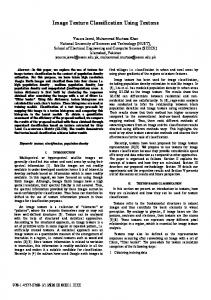
1. Introduction It was shown in [2] that there exists a strong correlation (R2 = 0.54, for the set of data used in this study) between the interstitial surface measured in kidneys biopsies and the Renal Function (RF). Interstitial surface was measured by stereological methods, i.e. by superimposing a grid of points to the image and counting manually the number of points falling into the interstitium (Fig. 1a). Results of these measures, obtained for 202 images taken from 35 biopsies, are shown in Fig.1b. The main disadvantages of this method are that it is time consuming and may vary depending on the observer. Colom�e-Serra [4] proposed an alternative approach which constisted of treating the image as a whole and not trying to segment it. A grey level granulometry was used which involved openings by hexagons of increasing size computed over the entire image. The result of this granulometry is a curve associated with each image. A multilinear regression was then obtained to establish a correlation with the renal function and to build an estimator. However, the approach proposed herein relies on segmentation of the images. Since it is impossible to decide whether a pixel belongs to a tubule or to the interstitium by considering only its grey level, textural information was used by computing a local granulometry over a small square window
2
C. GRATIN ET AL. RF vs Interstitium Area
140
120
100
80
60
40
20
0
a
0
5000
10000
15000
b
20000
25000
30000
Fig. 1. Measure of intersticial surface using point counting.
centered on each pixel. This granulometry forms vectors which were classi ed using a two (hidden) layer neural network.
2. Materials The data set used consists of 202 images of size 256 � 256 pixels taken from 35 biopsies (4 to 6 elds for each biopsy) with di�erent degrees of renal damage. Biopsies were stained with sirius red and digitized under polarized light. Images obtained with this technique are nearly binary, as can be seen in Fig. 2. Here tubules appear as white, non-textured and rather convex regions, while interstitium is limited to ne dark lines separating the tubules in the sanest biopsies (Fig. 2a). Progression
of tubulo-interstitial chronic renal damage is characterized by intersititial brosis, tubular atrophy and a decrease in the number of peritubular capillary [3]. As dam-
age increases, intersititium area tends to increase. Interstitial structures appear as textured regions, with no privileged orientation, in which it is not always easy to distinguish between interstitium and small size tubules or tubules in phase of decomposition (Fig. 2b and Fig. 2c).
3. Method 3.1. granulometry
A series of openings gamma [10] with a family of structuring elements B1 ; B1 ; : : :; B , is a granulometry if it satis es the following axiom [8]: n
8(i; j) i � j ) � : Bi
Bj
As the size of the structuring element increases, more and more details in the image are suppressed. Small structures present in the interstitium disappear after the rst openings, whereas large structures such as tubules remain nearly unchanged until large structuring elements are used. This phenomenon is illustrated in Fig. 3. Since
TEXTURE CLASSIFICATION USING N.N. AND LOCAL GRANULOMETRIES
a
b
3
c
Fig. 2. Images presenting an increasing renal damage: (a) sane, (b) & (c): pathological.
a
b
c
Fig. 3. Openings by disks of increasing radius: (a) 2, (b) 6 & (c) 15.
interstitial texture is isotropic, isotropic structuring elements were chosen. These were digital approximations of disks (B ) satisfying: 8(i; j) i � j ) (B ) = B : This property ensures that the granulometric axiom is ful lled (note that
(B +1 ) = B +1 is a su�cient condition as well). Interstitium texture is characterized by structures of small size, typically almost completely erased after an opening by a disk of radius 6. Therefore more importance was given to small size structures by putting in the granulometry ( ) more openings of small size. ( 1 2 3 4 6 10 15 25) was the family of closings chosen. i
j
Bi
Bi
i
j
i
i
3.2. Local Granulometry
In contrast to what was done in [4], the volume of the successive openings was not measured over the whole image. For each pixel x the volume V (x) was measured over a 17 � 17 pixels window centered on x. The volume (V (x)) =1 is an ndimensional vector at x, called here a local granulometry (LG). In the following we will only consider the granulometric spectrum of the image at x, i.e. the di�erential of the LG de ned as dV (x) = V (x) ? V ?1(x); i
i
i
i
i
i
;:::;n
4
C. GRATIN ET AL. 1 Local granulometry at x Local granulometry at y Local granulometry at z
0.8
0.6
0.4
0.2
0 0
a
5
10
b
15
20
25
30
Fig. 4. Local Granulometries of points situated in a tubule (x and z) and in the interstitium (y).
with V0 (x) being the volume measured on the initial image. Fig. 4b shows the granulometric curves dV (x) corresponding to the three points selected in Fig. 4a. We considered a 17 � 17 window large enough to contain textural information and small enough to remain \local". However, two neighboring pixels will have similar granulometric curves. Therefore, transitions from textured regions to non-textured regions tend to be smooth (and progressively smoother as the size of the window used increases). LG's are an e�cient tool to discriminate between textured and non-textured regions but it has a major disadvantage: only using this information usually makes it impossible to detect the ne dark interstitial lines that appear in normal biopsies between two tubules. Therefore, the grey level of pixel x was added to vector dV (x). The resulting n + 1 dimensional vector constituted the input to the neural network. i
i
3.3. Neural Network
A fully connected neural network with 9 input neurons, 10 neurons in a rst layer, 3 in a second layer and 1 neuron in the output layer, was formulated in the Aspirin language [7]. A C program was generated using Aspirin's compiler. A description of the network in Aspirin and it's graphical representation is shown in Fig. 5. We limited the dimension of the input space to 9 in order to reduce the number of examples necessary for the network to generalize. In fact, as noted in [6], if there are less examples than weights (i.e. connections), then the network tends only to memorize and reproduce these examples. A rst attempt was made with a one (hidden) layer network, but results improved signi cantly by adding a second layer. The dimension of the input space also in uences the number of neurons of the rst hidden layer. For example, a neuron calculating only the sign of the weighted sum of its inputs (i.e. the sigmoid function is replaced by a simple threshold) is in fact partitioning the space with a hyperplane into two half-spaces [9]. It follows that 10 (9+1) is the minimum number of neurons necessary to delineate a bounded region in the 9-dimensional input space. In this study about 150 points, taken from 8 images, were selected, classi ed manually and introduced in the network. A zero output value was assigned to
TEXTURE CLASSIFICATION USING N.N. AND LOCAL GRANULOMETRIES
5
DefineBlackBox Kidney { OutputLayer-> OUTPUT InputSize-> [9 x 1] Components-> { PdpNode OUTPUT [1 x 1] { InputsFrom-> Layer2 } PdpNode Layer2 [3 x 1] { InputsFrom-> Layer1 } PdpNode Layer1 [10 x 1] { InputsFrom-> $INPUTS } } }
a
b
Fig. 5. Aspirin description (a) and graphical representation (b) of the NN.
Fig. 6. Classi cation obtained for the images presented in Fig. 2.
interstitium while value of one was assigned to tubules. Weights were computed using a backpropagation learning algorithm with a 10 % output error.
4. Results Local granulometries for all the points of the 202 images were achieved with the help of ViLi software [1]. The output of the neural network was then computed and results were reassembled to form an image whose values were contained between 0 and 100. Pixels whose values were lower than 49 were classi ed as interstitium and pixels whose values were greater than 50 were classi ed as tubule. Fig. 6 illustrates the results obtained for the 3 images in Fig. 2. More interesting are the correlation factors between the interstitium area measured on all the images and the area determined manually, and between the mean of the interstitium area for all the images of a same biopsy and renal function. ? Automatic measure vs manual measure: R2 = 0.85, ? Mean of interstitium area (automatic) vs renal function: R2 = 0.53,
6
C. GRATIN ET AL. 45000 Automatic Measure vs Manual Measure
RF vs Automatic Measure
140
40000 35000
120
30000
100
25000
80
20000 60 15000 40 10000 20
5000 0
0 0
5000 10000 15000 20000 25000 30000 35000 40000 45000
a
0
5000
10000
15000
b
20000
25000
30000
Fig. 7. Results plotted as a function of the areas measured manually (a) and as a function of renal function.
? Mean of interstitium area (manual) vs renal function: R2 = 0.54.
Fig. 7 shows the distributions of these measures as a function of the areas measured manually (a) and as a function of renal function (b). These diagrams indicate that the proposed classi cation method reproduces the human process (R2 = 0.85) rather well and that it is nearly as accurate in the estimation of the renal function (R2 = 0.53 vs 0.54).
5. Comparison with other methods Neural Networks were not the only method investigated to segment interstitium. Two other more conventional methods, based on mathematical morphology operators, were also tried. They are described brie y below and their results can be compared with the results shown above. 5.1. Method using a simple threshold
As we noted earlier, images are nearly binary although some variations of the grey level's dynamic can be observed between two images taken from two distinct biopsies. The main issue is that interstitium does not restrict to dark regions but also includes textured regions where white small structures alternate with dark ones. The solution that we adopted was simply to threshold each image between 0 and N% of the mean and apply a morphological closing to the result using as a disk structuring element. The best result (in terms of maximum correlation with renal function) was obtained by setting N to 96% and the radius of the disk to 4. Fig. 8 shows the segmentation obtained with this method for the image of Fig. 2c (a) and renal function plotted as a function of the measures obtained for the 35 biopsies (b). The correlation factor was R2 = 0.52, which we consider to be a good result (although area tends to be over-estimated).
7
TEXTURE CLASSIFICATION USING N.N. AND LOCAL GRANULOMETRIES RF vs Automatic Measure
140 120 100 80 60 40 20 0 0
a
5000
10000
15000
b
20000
25000
30000
Fig. 8. Results of the threshold based method.
a
b
c
Fig. 9. Original Image (a), Regional Minima (b), Regional Minima whose dynamic is greater than 13 (c).
5.2. Method based on the dynamic of the minima
The second method is based on the observation that interstitial regions are regions containing many regional minima. Due to acquisition noise, there are also many minima inside the tubules but the former and the latter can be easily discriminated using a criteria of dynamic [5]. Fig. 9 illustrates this phenomena: In (b) tubules contain many minima but in (c) none of dynamics greater than 13. The solution retained was thus to compute the dynamic of the minimaand threshold the resulting image between N and 255 (the maximum grey level value). Interstitium was then reconstructed by applying a morphological closing using a disk as structuring element. The best result (in terms of maximum correlation with the renal function) was obtained by setting N to 13 and the radius of the disk to 5. Fig. 10 shows the segmentation obtained with this method for the image of Fig. 2c (a) and the renal function plotted as a function of the measures obtained for the 35 biopsies (b). The correlation factor was R2 = 0.54. This is equivalent to the correlation obtained with the manual method.
8
C. GRATIN ET AL. RF vs Automatic Measure
140 120 100 80 60 40 20 0
a
0
5000
10000
15000
b
20000
25000
30000
Fig. 10. Results of the dynamic based method.
6. Conclusion Three methods for the automatic segmentation of intersititium in images of kidneys' biopsies have been presented, with particular emphasis on a method achieving pixel classi cation through the use of a Neural Network. All three methods reproduce the results obtained by manual classi cation rather well. The use of a neural network seems promising since it does not require any size or threshold parameter. Moreover it is a \dynamic" system that can be modi ed through learning if it appears to give unsatisfactory results for some images. Clinical implementation of the three methods is in progress and should provide data to validate or invalidate the results presented here.
References 1. Vili (vision lisp). Image Processing Functions. User & Programmer Manual. Technical report, Universitat Aut�onoma de Barcelona, 1993. 2. D. Ser�on et al. Relationship between donor renal interstitial surface and post-transplant function. Nephrol Dial Transplant, 8:539{543, 1993. 3. F. Moreso et al. Quanti cationof interstitial chronic renal damage by means of image analysis. Submitted, 1994. 4. M.F. Colom�e-Serra et al. Image analysis: utility of grey level granulometry to measure renal intersticial chronic damage. In Proc. IEEE Int. Conf. Medicine, pages 1934{1935, 1993. 5. M. Grimaud. La g�eod�esie num�erique en morphologie math�ematique. Application �a la d�etection automatique de microcalci cations en mammographies num�eriques. PhD thesis, Ecole des Mines de Paris, D�ecembre 1991. 6. K.J. Lang, A.H. Waibel, and G.E. Hinton. A time-delay neural network architecture for isolated word recognition. Neural Networks, 3:23{44, 1990. 7. Russel R. Leighton. The aspirin/migraines neural network software. User's Manual. Release V6.0. Technical report, MITRE Corporation, 1992. 8. G. Matheron. Random Sets and Integral Geometry. New York: Wiley, 1975. 9. L.I. Perlovsky. Computational concepts in classi cation: Neural networks, statistical pattern recognition, and model-based vision. Journal of Mathematical Imaging and Vision, 4:81{110, 1994. 10. J. Serra. Image analysis and mathematical morphology. Academic Press, 1982.