Classification of Textures Using Filter Based Local Feature Extraction

MATEC Web of Conferences 75, 03001 (2016)

DOI: 10.1051/ matecconf/20167503001

ICMIE 2016

Classification of Textures Using Filter Based Local Feature Extraction 1

Veysel Gokhan Bocekci and Kazim Yildiz

2

1

Marmara University, Technology Faculty, Electric and Electronic Engineering, 34722 Istanbul, Turkey Marmara University, Technology Faculty, Computer Engineering, 34722, Istanbul, Turkey

2

Abstract. In this work local features are used in feature extraction process in image processing for textures. The local binary pattern feature extraction method from textures are introduced. Filtering is also used during the feature extraction process for getting discriminative features. To show the effectiveness of the algorithm before the extraction process, three different noise are added to both train and test images. Wiener filter and median filter are used to remove the noise from images. We evaluate the performance of the method with Naïve Bayesian classifier. We conduct the comparative analysis on benchmark dataset with different filtering and size. Our experiments demonstrate that feature extraction process combine with filtering give promising results on noisy images.

1 Introduction The feature extraction and identification of the texture is a challenging duty in computer vision, especially number of features. It is known texture analysis is a kind of problem in literature. In feature extraction process, so many methods were designed like filter banks [1], cooccurrence statistics [2] and hidden Markov models [3]. These all application are based on two dimensional surfaces. To overcome of the problem like rotation, scale and illumination, the texton based approaches were designed [4-6]. Images are served as histograms of the discrete vocabulary of features. Local binary pattern (LBP) is most well-known and popular descriptor because of its computational simplicity, robustness of the gray scale changes and promising performance [7]. There are also some limitations to using it, for instance the descriptor is not invariant to rotation, the size of the features are growing exponentially and increase the time complexity of the algorithm. The other reason is structural information which is taken from texture is limited [8]. For improving of the algorithm performance and overcome of the limitations, there are some modifications on it. LBP descriptors are designed and the local orientation is completely removed [7]. LBPHistogram Fourier based algorithm is designed by Zhao and friends [9]. The mentioned algorithm interested in magnitude spectrum of the transform. Multiresolution information is taken from images with the help of LBP, various granularities can be captured [10]. Liao and friends are designed dominant LBP to choose the outlier features from images [11]. Guo proposed a method to overcome of the feature increasing problem which is fisher criterion based algorithm [12]. We designed filter based LBP to extract features from images. The Brodatz

dataset is used for evaluate the performance of the method. It is one of the first and common datasets which have been used in texture analysis. Naïve Bayesian algorithm is used in classification process. The classification algorithm is effective on complex problems when comparing the neural network classifier that is the reason why we choose it as a classifier. The paper is organized as follows: In Section 2, the MATERIALS and method are given. Results of the experiments and finally conclusion part is given. Finally conclusion is given.

2 Materials and method In this part we give information about the details of proposed approach and using algorithms. First LBP is described, then median filter and classification process are introduced. 2.1 Feature extraction with LBP Central pixel and its neighbors difference is taken by LBP which operates in a local circular [13]. It is referred in 1; p 1 1 g p p LBPR , P s ( g p g c )2 , s ( g p g c ) (1) p 0 0 g p

Central pixel and its neighnbors are represented with gc and gp which are the gray value. Neighbor index is determined by p and radius of the circular neighborhood is R. Number of the neighbors are identified by P. The coordinates of uniformly spaced circular neighbourhood are determined as (x+Rcos(2πp/P), y−Rsin(2πp/P))(x+Rcos(2πp/P), y−Rsin(2πp/P)) for p=0,1,2…P−1p=0,1,2…P−1. [8].

© The Authors, published by EDP Sciences. This is an open access article distributed under the terms of the Creative Commons Attribution License 4.0 (http://creativecommons.org/licenses/by/4.0/).


DOI: 10.1051/ matecconf/20167503001

ICMIE 2016 probability. For parameter estimation, NB uses maximum likelihood method [20]. For a classifier, a conditional model is referred in (4);

The Figure 1 shows how the LBP works. Label’s partitions is computed after the thresholding process which can be used as a texture descriptor. Local primitives are encoded via each histogram partition.

p(CIX1 ,..... X n )

(4)

where C is a class and X is a feature variable. Feature can take large number values, when n is grow then basic model should be infeasible. It is referred in (5); Figure 1. Scheme of local binary pattern.

p (CIX 1 ,..... X n )

2.2 Median filter Median filter is used as a non-linear filter. Generally it is used for removing noise [14]. In this filter, the median value is used for the value of corrupted pixel in noisy image of the corresponding window. This reference pixel describes the value which is in the middle position of any sorted matrix [15]. For example the gray levels of any pixel value, in any window (wx) of size nxn are represented by x1, x2, x3,…xn. After sorting it should be ascending or descendingxi1ı xi2ı xi3Ăıxin. Equation 2 value of the median; X i ( n 1) n is odd

p (c ) p ( X 1 .... X n IC )

(5)

p ( X 1 ,.... X n )

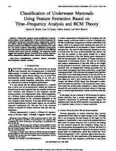
3 Results and discussion All the codes and experiments were developed using Matlab2015a. In this part, information of the dataset and obtained results are given. 3.1. Data source There are so many number of texture databases on the net for comparison the algorithms performance. In this paper we used Brodatz texture album. It has been used much and one of the first dataset which includes textures of natural scenes and materials such as bark, sand and grass. The original images of the dataset are not digital format [21]. The images in this paper should be find in [22]. We used thirteen classes from texture album. Figure 2 shows the dataset which includes classes

; 2 (2) M x Median( wx )

1 X n X n n is even i ( ) 1 2 i ( 2 ) 2

There is so many different median filter based image denoising algorithm in literature. In this paper we used MATLAB median filter to remove the noise and outlier points from image. 2.3 Wiener filter Wiener filter builds an optimal estimate of original image. The difference between original image and estimate is aimed to enforce a smallest mean square error [16]. It is used as an optimum filter which minimize mean square error. It has capability of handling both degradation function and also removing the noise [17]. In general the best way to reconstruction of a noisy signal is using wiener filter because of its optimal and adaptive ability. The aim of the filter is minimize the least square error is referred in (3) [18]; 2 min E fˆ f (3)

Figure 2. Brodatz texture album which has 13 classes.

3.2 Comparison of the performance

where f represents the original image and restored image.

We proposed two different approaches. The dataset for the experiment is divided two part. First we used half of the dataset as train and the rest of it for test. For second approach to show the robustness of the proposed approach we decreased the number of train images. 52 images are used for train 156 images are used for test. Also we test the algorithm performance to add three different noises to both train and test images before filtering part which are Gaussian, speckle and Poisson. After adding noise, filtering part is applied to the images. The feature extraction part come after this. Obtained feature vector is used for the classification process. Figure 3 shows the example of adding noises to image.

is the

2.4 Naïve Bayes classifier In pattern recognition, the classification process is an important issue. There are so many different algorithms such as nearest neighbor, decision tree and neural network. Naïve Bayes (NB) is based on Bayesian theorem which has probabilistic model [19]. NB takes into account each features to subscribe independently to

2


DOI: 10.1051/ matecconf/20167503001

ICMIE 2016 Table 2 shows the classification accuracy on image dataset with speckle noise (SN). The original classification with noise images is averagely 88%. Wiener filtering help the process with ten point increase. It is really so effective of the removing noises from images because of the adaptive structure. The obtained results with median filter is just about giving four point improvement. The average performance of the classification is 98.078 with wiener filter.

a b c d Figure 3. Original image (a) Gaussian noise added (b) speckle noise added (c) Poisson noise added (d)

After noise adding, for removing the noise we apply the median and wiener filter to the images respectively. The example of the application is shown in Figure 4. From images it can be seen the effective of the noises. Median and wiener filters improvement stage also is shown. Because of the its adaptive structure wiener filter does more soft effects to remove noises from images.

a

b

d

Table 2. The classification accuracy with speckle noise and filter. SN Case 1 Case 2 Case 3 Case 4 Case 5 Average

c

e

86.54 88.46 91.35 88.46 84.62

MF 3x3 90.38 86.54 93.27 91.35 88.46

MF 5x5 92.31 91.35 93.27 95.19 91.35

MF 10x10 91.35 93.27 91.35 93.27 89.42

WF 3x3 93.27 94.23 99.04 92.31 94.23

WF 5x5 98.08 97.12 100 99.04 96.15

87.88

90

92.69

91.73

94.61

98.07

Table 3 shows the classification accuracy on image dataset with Poisson noise (PN). Actually with Poisson noise the classification is about the 94% averagely. It is not so effective to disturb the structure of the image. However filtering process should avoid these situation. And the classification is goes up to 99%. The average performance of the classification is 98.078 with wiener filter.

f

Table 3. The classification accuracy with Poisson noise and filter.

g h k Figure 4. (a) Image with Gaussian noise (b) noise removing with wiener filter (c) noise removing with median filter (d) image with speckle noise (e) noise removing with wiener filter (f) noise removing with median filter (g) image with Poisson noise (h) noise removing with wiener filter (k) noise removing with median filter

PN Case 1 Case 2 Case 3 Case 4 Case 5 Average

96.15 93.27 94.23 93.27 96.15 94.61

MF 3x3 98.08 99.04 96.15 99.04 99.04 98.27

MF 5x5 99.04 98.08 97.12 98.08 99.04 98.27

MF 10x10 99.04 99.04 98.08 98.08 98.08 98.46

WF 3x3 100 99.04 99.04 99.04 100 99.42

WF 5x5 99.04 99.04 100 99.04 98.08 99.04

We try our proposed work on different conditions. Five different train and test images are selected for experimental process. The classification accuracy on image dataset with Gaussian noise (GN) is shown in Table 1. For comparing the algorithm performance five different train and test image subset is selected. Also different size of the filter is applied to the images before classification to compare the effect on it. Averagely wiener filter with the size 5x5 is the most powerful filter to remove the noise before the classification when comparing the median filter (MF). The average performance of the classification is 99.232 with wiener filter (WF).

To compare the effectiveness of the algorithm on the process, we reduce the number of training images. 52 images are selected for training stage randomly and the rest of them are used for testing. For all process the wiener filter so effective for removing noise. The averagely obtained results are about 88% accuracy for classification which can be seen in Table 4. Our proposed approach makes improvement when comparing the nonfiltered results.

Table 1. The classification accuracy with Gaussian noise and filter.

Table 4. The classification accuracy with small training set usage.

GN Case 1 Case 2 Case 3 Case 4 Case 5 Average

92.31 83.65 88.46 87.5 87.5 87.88

MF 3x3 94.23 93.27 92.31 93.27 93.27 93.27

MF 5x5 96.15 96.15 94.23 97.12 95.19 95.76

MF 10x10 97.12 98.08 92.31 94.25 95.19 95.39

WF 3x3 91.35 96.15 97.12 99.04 96.15 95.96

WF 5x5 98.08 100 99.04 99.04 100 99.23

No filter Gaussian 63.64 noise Speckle 86.3 noise Poisson 73.68 noise

3

MF 3x3

MF 5x5

MF 10x10

WF 3x3

WF 5x5

78.21

83.22

76.92

79.71

90.97

88.31

88.44

86.54

91.39

85.92

64.9

80

85.26

72.19

86.45


DOI: 10.1051/ matecconf/20167503001

ICMIE 2016

4 Conclusion In this paper we described a framework which is a filtering based feature extraction process. The main idea of the paper to show the robustness of the feature extraction and classification process with additive noise. We choose different types of noise to compare the algorithm performance. For feature extraction process the common method which is LBP used. LBP is local texture feature extraction method and it’s commonly used in texture feature extraction process. Brodatz texture images are used to test proposed model efficiency. The dataset is divided into two parts. For removing noise, the wiener and medina filter is used respectively to compare the efficiency of them. Both of them known as effective on noise and outlier pixels on images. In this work wiener filter is so effective to remove the noise form images because of its adaptive structure. Naïve Bayes algorithm is used in classification process. Averagely 99% classification result is taken with wiener filter usage during removing noise process. Non filtering classification accuracy is decreased when using training set is reduced. Averagely filtering classification accuracy is about 88%. Our proposed approach shows promising results for both situation. For future work we should try our method on different types of datasets. To show the filtering part efficiency it will design new types of filters and it is going to try under different noise conditions.

8.

9.

10.

11.

12.

13.

14.

References 1.

2.

3.

4.

5.

6.

7.

Randen, T. and Husoy, J.H., Filtering for texture classification: A comparative study. Pattern Analysis and Machine Intelligence, IEEE Transactions on, (1999). 21(4): pp. 291-310 Haralick, R.M., Statistical and structural approaches to texture. Proceedings of the IEEE, (1979). 67(5): pp. 786-804 Chen, J.-L. and Kundu, A., Rotation and gray scale transform invariant texture identification using wavelet decomposition and hidden Markov model. Pattern Analysis and Machine Intelligence, IEEE Transactions on, (1994). 16(2): pp. 208-214 Lazebnik, S., Schmid, C., and Ponce, J., A sparse texture representation using local affine regions. Pattern Analysis and Machine Intelligence, IEEE Transactions on, (2005). 27(8): pp. 1265-1278 Mehta, R. and Egiazarian, K., Texture Classification Using Dense Micro-block Difference (DMD), in Computer Vision--ACCV 2014. (2014), Springer. pp. 643-658. Varma, M. and Zisserman, A., A statistical approach to texture classification from single images. International Journal of Computer Vision, (2005). 62(1-2): pp. 61-81 Ojala, T., Pietikäinen, M., and Mäenpää, T., Multiresolution gray-scale and rotation invariant

15. 16.

17.

18.

19.

20.

21.

22.

4

texture classification with local binary patterns. Pattern Analysis and Machine Intelligence, IEEE Transactions on, (2002). 24(7): pp. 971-987 Mehta, R. and Egiazarian, K., Dominant Rotated Local Binary Patterns (DRLBP) for texture classification. Pattern Recognition Letters, (2016). 71: pp. 16-22 Zhao, G., et al., Rotation-invariant image and video description with local binary pattern features. Image Processing, IEEE Transactions on, (2012). 21(4): pp. 1465-1477 Qian, X., et al., PLBP: An effective local binary patterns texture descriptor with pyramid representation. Pattern Recognition, (2011). 44(10): pp. 2502-2515 Liao, S., Law, M.W., and Chung, A., Dominant local binary patterns for texture classification. Image Processing, IEEE Transactions on, (2009). 18(5): p. 1107-1118 Guo, Y., et al., Descriptor learning based on fisher separation criterion for texture classification, in Computer Vision–ACCV 2010. (2010), Springer. pp. 185-198 Tai, S.-C., Chen, Z.-S., and Tsai, W.-T., An automatic mass detection system in mammograms based on complex texture features. Biomedical and Health Informatics, IEEE Journal of, (2014). 18(2): pp. 618-627 Gupta, V., Chaurasia, V., and Shandilya, M., Random-valued impulse noise removal using adaptive dual threshold median filter. Journal of Visual Communication and Image Representation, (2015). 26: pp. 296-304 Gonzalez, R.C. and Woods, R.E., Digital image processing. (2002): Prentice hall Upper Saddle River Jog, A. and Halbe, S., Multiple Objects Tracking Using CAMShift Algorithm and Implementation of Trip Wire. International Journal of Image, Graphics and Signal Processing, (2013). 5(6): p. 43 Mane, S.A. and Kulhalli, K., Mammogram Image Features Extraction And Classification For Breast Cancer Detection. (2015) Jin, F., et al., Image Restoration Based on Wiener Filtering Journal of communication university of china (Science and Technology), (2011). 4: p. 005 Zhou, X., et al., Detection of pathological brain in MRI scanning based on wavelet-entropy and naive bayes classifier, in Bioinformatics and biomedical engineering. (2015), Springer. pp. 201-209 Platt, J.C., Cristianini, N., and Shawe-Taylor, J. Large Margin DAGs for Multiclass Classification. in nips. (1999) Tuceryan, M. and Jain, A., Textures: a photographic album for artists and designers. (1966), Dover Publications The USC-SIPI, I.d. http://sipi.usc.edu/database/. (1977) [cited 2016 November]