Polyline Feature Extraction for Land Cover Classification using Hyperspectral Data Alexandre Henneguelle, Joydeep Ghosh, and Melba Crawford Department of Electrical and Computer Engineering, Center for Space Research The University of Texas at Austin, TX, USA 78712
[email protected],
[email protected],
[email protected]
Abstract. Prediction of landcover types from airborne/spaceborne sensors is an important classification problem in remote sensing. Due to recent advances in sensor technology, it is now possible to acquire hyperspectral data simultaneously in ∼200 bands, each of which measures the integrated response of a target over a narrow window of the electromagnetic spectrum. This unprecedented spectral resolution can provide vastly improved mapping of several types of landcover and monitoring of ecological changes. However, the increased dimensionality also constitutes a challenge in terms of storage and analysis. This paper presents a Polyline Feature Extraction (PFE) technique that exploits the spectral correlations between certain adjacent bands in hyperspectral data, to reduce dimensionality without sacrificing discrimination power. It uses an interpretable piecewise linear representation of the data that is somewhat robust to environmental changes. Using the Binary Hierarchical Classifier Framework for multi-class problems, PFE’s effectiveness is demonstrated on two large hyperspectral datasets obtained over the Texas and Florida coasts respectively.
Keywords: hyperspectral data analysis, machine learning, classification, remote sensing, knowledge extraction
1
Introduction
The increasing availability of data from hyperspectral sensors has generated tremendous interest in the remote sensing community because these instruments characterize the response of targets (spectral signatures) with greater detail than traditional sensors and thereby can potentially improve discrimination between targets[1, 2]. A common application is to determine the land cover label of each (vector) pixel by using labeled training data (ground truth), X, to estimate the parameters of the label-conditional probability density functions, P (x1 , x2 , . . . , xD |Li ), i = 1, . . . , C, or to directly estimate the aposteriori class probabilities. Unfortunately, classification of hyperspectral data is challenging for several reasons. The dimensionality of the data (D) is high (∼ 200), as contrasted with traditional optical “multispectral” sensors that acquire data in a
few (< 10) broad channels on the order of a hundred nanometers in width. Thus any data analysis is potentially faced with the “curse of dimensionality”[3]. The sensor measurements obtained from a given land cover type can vary somewhat over time and space, and thus the class-conditional likelihoods can vary from image to image. The number of classes C is often in the teens, and obtaining labeled data is expensive and time consuming because it either involves field campaigns or manual interpretation of high resolution imagery. However, hyperspectral data tend to be correlated both spectrally and spatially, and these two properties can often be exploited to make the classification problem more tractable. In this paper, we propose a feature extraction algorithm that exploits the the fact that bands that are spectrally “near” each other tend to be highly correlated, to obtain an effective feature extraction technique for hyperspectral data. In section 2 we briefly describe previous work on feature extraction for such data. The proposed method is described in section 3, and experimental results are presented in section 4.
2
Feature Extraction from Hyperspectral Data
Hyperspectral sensors simultaneously acquire information in hundreds of spectral bands. A hyperspectral image is essentially a three-dimensional array I(p, q, d), where (p, q) denotes a pixel location in the image, and d denotes a spectral band (wavelength). The value stored at I(p, q, d) is the response (reflected or emitted energy) from the pixel (p, q) at a wavelength corresponding to spectral band d. The input space for a hyperspectral data (classification problem) is an ordered vector of real numbers of length D, the number of spectral bands, wherein the response of bands that are spectrally “near” each other tend to be highly correlated within certain regions of the spectrum. Analysis of hundreds of simultaneous channels of data necessitates the use of either feature selection or extraction algorithms prior to classification. Feature selection algorithms for hyperspectral classification are costly, while feature extraction methods based on Karhunen Loeve (KL) transforms, Fisher’s discriminant, or Bhattacharya distance cannot be used directly in the input space because the covariance matrices required by all these approaches are highly unreliable, given the ratio of the amount of training data to the number of input dimensions. The results are also difficult to analyze in terms of the physical characteristics of the individual classes and are not generalizable to other images. Several authors have proposed approaches for extracting features from remotely sensed hyperspectral data[4, 5, 4, 2]. Lee and Landgrebe[6, 7] proposed methods for feature extraction based on decision boundaries for both Bayesian and neural network based classifiers. In these methods, a classifier is first learned for a two-class problem in the input space. A decision boundary is computed by moving along the closest samples in the two classes, and a vector normal to the decision boundary is noted. Eigenvectors of the decision boundary feature matrix formed by collection of these normal vectors yield the direction of projection
for the two-class problem. The C-class problem is then solved using a (weighted) sum of the decision boundary feature matrices. Jia and Richards proposed a Segmented Principal Components Transformation (SPCT) that expliots the observation that the original input features - the bands of the hyperspectral data - that are spectrally close to one another, tend to be highly correlated[8, 5]. Edge detection algorithms are used to transform the original D individual bands into subsets of adjacent bands that are highly correlated, based on the estimated population correlation matrix. From each subset, the most significant principal components are selected to yield a feature vector that is significantly smaller in dimension than D. Although this approach exploits the highly correlated adjacent bands in hyperspectral data, it does not guarantee good discrimination capability because the Principal Component Transform preserves variance in the data rather than maximizing discrimination between classes. Additionally, the segmentation approach of SPCT is based on the correlation matrix over all of classes, and thus loses the often-significant variability in the class conditional correlation matrices. Subsequently, Kumar et al. proposed band combining techniques inspired by Best Basis functions[1]. Adjacent bands were selected for merging (alt. splitting) in a bottom-up (alt. top-down) fashion using the product of a correlation measure and a Fisher based discrimination measure[4]. Although these two methods utilize the ordering of the bands and yield excellent discrimination, they are computationally intensive. They also focus essentially on discrimination rather than interpretability or stability under changing (atmospheric, time of day. etc.) conditions. The polyline approximation feature extractor described in the next section can be viewed as another development of the concept of “Best-Bases”, with a different emphasis.
3
The Polyline Feature Extraction (PFE) Technique
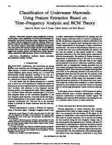
The key idea behind PFE is to treat the wavelength ordered bands of hyperspectral data as a “time series”, with spectral ordering substituting for time. Dependencies among neighboring spectral bands thus tranlate into temporal correlations, and there is a vast literature on piecewise linear representations of time series that one can now draw on. After examining a large quantity of hyperspectral data from a variety of landcovers (see Figure 1, for example), , we felt that a piecewise linear description is suitable as it captures the essential discriminating spectral features in 15-20 attributes that are reasonably interpretable. This judgement is validated by the empirical results given later. There are two main steps in PFE: (i) Determine suitable break-points, i.e., locations where the behavior of the signatures changes significantly, and (ii) find a good representation of the data in each segment demarcated by adjacent break-points. 3.1
Break-Point Detection
For the first step, we investigated three alternatives. The description of these three alternatives below is taken directly from [18], which also contains further
600
Class 2
Class 1
600 400 200 0
20
40
60
80
100
400 200
120
20
40
60
80
100
120
20
40
60
80
100
120
20
40
60
80
100
120
20
40
60
80
100
120
20
40
60
80
100
120
Class 4
Class 3
3000 2000 1000
3000 2000 1000
20
40
60
80
100
120
4000
6000
Class 6
Class 5
5000
4000
20
40
60
80
100
120 5000 4000
3000
Class 8
Class 7
4000
2000 1000
3000 2000 1000
20
40
60
80
100
120
6000
4000
Class 10
Class 9
2000 1000
2000
Class 11
3000
4000 2000
3000 2000 1000
20
40
60
80
100
120
20
40
60
80
100
120
4000 3000 2000 1000
Fig. 1. Signatures of the classes in the HYMAP data set.
details about them. (i) Sliding Window Approach: The Sliding Window approach involves anchoring the left point of a potential segment as the first data point of a time series, then attempting to approximate the data to the right with increasingly longer segments. At some point i, the error (typically measured as L∞ or least squares) for the potential segment is greater than the user-specified threshold, so the subsequence from the anchor to i − 1 is transformed into a segment. The anchor is moved to location i, and the process repeats to determine the next segment. This approach is attractive because of its great simplicity, intuitiveness, and the fact that it is an online algorithm. Such characteristics have made this technique extremely popular for stock market analysis, as well as in the medical community (where it is known as FAN or SAPA), since patient monitoring is inherently an online task [9, 10]. Several variations and optimizations of the basic algorithm
have been proposed over the years [9]. However, the Sliding Window algorithm can give pathologically poor results under some circumstances. Shatkay and Zdonik [11] noticed the problem and gave elegant examples and explanations. They considered three variants of the basic algorithm, each designed to be robust to a certain case, but they also underline the difficulty of producing a single variant of the algorithm which is robust to arbitrary data sources. (ii) Top-Down Approach: Here, every possible partitioning of the full data sequence is considered, and the split occurs at the best location. Both subsections are then tested to determine whether their approximation error is below some user-specified threshold. If not, the algorithm recursively continues to split the subsequences until each of the segments have approximation errors below the threshold. Variations on the Top-Down algorithm (including the 2-dimensional case) were independently introduced in several fields in the early 1970s. Most researchers in the machine learning/data mining community are introduced to the algorithm in the classic textbook by Duda and Hart, which calls it Iterative End-Points Fits [12]. In the data mining community, the algorithm has been used by [13] to support a framework for mining sequence databases at multiple abstraction levels. Shatkay and Zdonik [11] used it (after considering alternatives such as Sliding Windows) to support approximate queries in time series databases. Lavrenko et al. [14] used the Top-Down algorithm to support the concurrent mining of text and time series. They attempted to discover the influence of news stories on financial markets. Their algorithm contains some interesting modifications including a novel stopping criteria based on the t-test. (iii) The Bottom-Up Approach: This is a natural complement to the TopDown approach, and starts with each point belonging to its own segment. Next, the cost of merging each pair of adjacent segments is calculated, and the algorithm begins to iteratively merge the lowest cost pair until a stopping criteria is met. In data mining, the algorithm has been used extensively by [15–17] to support a variety of time series data mining tasks. Polyline Algorithm. Given that the class signatures are computed, the desired polyline algorithm is off-line. As a consequence, any of the three approaches described above can be applied. Preliminary experiments showed that the sliding window approach yielded relatively poor quality, so this option was not investigated further. Moreover because a small number of segments are desired, a top-down approach is advantageous as compared to bottom-up which is more computationally expensive as we start with over 100 segments. The chosen algorithm is: 1. Initialize the set of break points: B = {1, D} 2. For each class ω ∈ Ω: – Find the piecewise linear approximation of the signature for the current set of break points – Find the error Eωb induced by the approximation for each individual band b ∈ [1, D] 3. Find the best break point at this level: b0 = arg max max Eωb b∈1...D ω∈Ω
(1)
4. Update the set of control points: B = B ∪ b0 5. Return to step 2 if more break points are needed. In this work, the error Eωb is defined as the distance between the signature of class ω and the best fit line (within the segment containing b) normalized by the standard deviation of class ω at the band b. 3.2
Segment Representation
Linear representation of a segment is usually done via linear interpolation, which is simple and automatically aligns the end-points of consecutive segments, or by linear regression, typically using a least squares fit, or robust statistics technques such as trimmed-means [19] if outliers are a problem. For PFE, we ended up representing each segment S[a : b] by two features: (i) Midpoint of the segment: X 1 xi b − a + 1 i=a b
Ma,b (x) =
(2)
(ii) Slope of the segment: Sa,b (x) = xb − xa
(3)
This representation appears to be a reasonable compromise between linear interpolation and linear regression in the sense that it is more sophisticated than linear interpolation and less computationally demanding than linear regression. Equally important, we noticed that the slope, which carries shape information, is often the most important discriminator between classes and shows relatively less variation within the same class, i.e., different pixels belonging to the same land-cover may have somewhat displaced spectra but there is not much change in the slope values. 3.3
Classifier Design
The 2N features from N segments obtained by a PFE can be further reduced via feature selection or extraction methods. Moreover, these features can be used by a wide variety of classifiers. Note that the suitability of a feature reduction technique is in general dependent on the classifier to be used in the next stage, though for speedup, often these two stages are decoupled. Since interpretability is a key consideration, we preferred feature selection. A greedy forward selection approach was found to perform well for hyperspectral data. Then we need to design a classifier that can effectively deal with ∼10 classes, and ∼10 features. Our previous work showed that the Binary Hierarchical Classifier (BHC) is very suitable for hyperspectral data, outperforming a large number of alternatives including maximum-likelihood classifiers, multi-layered perceptrons, local discriminant bases, and (generalized) support vector machines [4, 20]. Thus this became a natural choice to be adapted for PFE. We briefly describe the BHC below, for details, see [4].
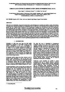
The top down BINARY HIERARCHICAL CLASSIFIER (TD-BHC) framework was introduced in [4] as a way of recursively decomposing a C-class problem into C − 1 two-(meta)class problems. It results in a multi-classifier system with C − 1 classifiers arranged as a binary tree. The root classifier tries to optimally partition the original set of classes into two disjoint meta-classes while simultaneously determining the Fisher discriminant that separates these two subsets. This procedure is recursed, i.e., the meta-class Ωn at node n is partitioned into two meta-classes, (Ω2n , Ω2n+1 ), until the original C classes are obtained at the leaves[4]. Fig. 2 shows an example of a C-class BHC. Note that the partitioning of a parent set of classes into two sets of metaclasses is not arbitrary, but is obtained through a deterministic annealing process that encourages similar classes to remain in the same partition. The tree structure also allows the easier discriminations to be accomplished earlier[21].
W1 = {1, … , C}
1
Internal node
W2 = {1, C-1}
W3 = {2, … , C-2, C}
2
3 W6 = {5, 9}
1 W4 = {1}
6
C-1
WA = {3, 6, C}
W5 = {C-1}
A Leaf node
5
9
W12 = {5}
W13 = {9}
W2A+1 = {3, C}
2A+1
6 W2A = {6}
3
C
W4A+2 = {3}
W4A+3 = {C}
Fig. 2. An example of a BINARY HIERACHICAL (multi)-CLASSIFIER for solving a C-class problem. Each internal node n comprises of a feature extractor, a classifier, a left child 2n, and a right child 2n + 1. Each node n is associated with a meta-class Ωn .
Subsequently, a bottom-up version (BU-BHC) was developed based on an agglomerative clustering algorithm used for recursively merging the two most similar meta-classes until only one meta-class remains[22]. Fisher’s discriminant was again used as the distance measure for determining the order in which the classes are merged. The bottom-up procedure is computationally more expensive than the top-down version, but sometimes produces even better results, although it is locally more greedy. PFE can be incorporated into the generic BHC framework in two different ways: – Global Preprocessing: PFE is applied over all the classes and provides the same partition of the spectrum for all the two (meta)-class subproblems. – Modular Preprocessing: PFE is applied separately to each two (meta)-class subproblem, so that the decomposition of the spectrum is customized for each module. Both alternatives are examined in the empirical studies presented in the next section.
4 4.1
Experimental Results Bolivar Peninsula (HYMAP)
We performed experiments using HYMAP (Hyperspectral Mapper) reflectance data acquired in 1999 over the Bolivar Peninsula which is located at the mouth of Galveston Bay in the Texas Gulf coast. The HYMAP data are formed of 126 bands with wavelengths ranging from 0.44µm and 2.48µm. As recommended in [23], we eliminated bands 63, 64, 95 and 126 because of their low signal-tonoise ratio. For classification purposes, 11 classes listed in Table 1 were defined. The labelled samples were randomly partitioned into 50% training and 50 % test sets. The signatures of the twelve classes are depicted in Figure 1. The labelled samples were randomly partitioned into 50% training and 50% test sets for each of the ten experiments. The classification results reported in Table 2 show that PFE results are just below but comparable to the best results reported so far on this dataset [4]. Also note that the modular preprocessing gives better results than the global preprocessing. The main advantage of the PFE comes from its potential for interpretability. For simplicity, the analysis of the domain knowledge is made in the case of global preprocessing. First we observe that the partitions of the spectrum are quite stable between runs. The most common partition is indicated in Table 3. Completely adapted to the physionomy of the signatures, this decomposition seems very helpful for the purpose of interpretation. The hierarchy constructed for the partition of spectrum given in Table 3 is presented in Figure 3 and the features selected at each node of this hierarchy are reported in Table 4. One
ID 1 2 3 4 5 6 7 8 9 10 11
Class Name Number of examples Water 1019 Low proximal marsh 1127 High proximal marsh 910 High distal marsh 752 Sand Flats 148 Agriculture1 (pasture) 3073 Trees 222 General uplands 704 Agriculture2 (bare soil) 1095 Transition zone 114 Pure Salicornia 214
Table 1. The eleven classes in HYMAP hyperspectral data set.
can notice that features referred as “slope” are often selected for discrimination between classes, which proves that the shape characteristics of the signatures are very important for classification.
BU-BHC TD-BHC PFE-G 98.11 (0.18) 98.19 (0.48) PFE-M 98.55 (0.36) 98.35 (0.69) Table 2. Test set accuracies and standard deviations on the HYMAP dataset.
4.2
Cape Canaveral (AVIRIS)
The efficacy of the proposed feature extraction algorithm is also shown by experiments using a 175 band hyperspectral data set acquired by the NASA AVIRIS spectrometer over Kennedy Space Center in Florida. In this case, we worked with the radiance data. For classification purposes, 13 landcover types were identified and the labelled samples were randomly partitioned into 50% training and 50 % test sets. The evaluation is carried out analogously to that in Section 4.1. Results in Table 5 support conclusions similar to those indicated by Table 2. For lack of space, we are omitting details about class distributions, signatures and features extracted, and simply remark that once again, the features referred as “slope” are selected quite often, further underscoring the importance of such shape characteristics for classification.
Midpoint Slope Bands Spectral Range (nm) 1 2 1-8 441 - 549 3 4 8 - 16 549 - 671 5 6 16 - 19 671 - 717 7 8 19 - 58 717 - 1177 9 10 58 - 62 1177 - 1346 11 12 62 - 63 1346 - 1429 13 14 63 - 65 1429 - 1456 15 16 65 - 83 1456 - 1691 17 18 83 - 93 1691 - 1966 19 20 93 - 122 1966 - 2462 Table 3. Decomposition of the spectrum obtained on the HYMAP dataset with the Polyline Algorithm.
Node 21 20 19 18 17 16 15 14 13 12
Selected Features 8, 1, 2, 13, 10 5, 15, 17 6, 1, 7, 8 12, 1, 3, 5, 7, 4, 6, 2 16, 12 14 13 5, 6, 7, 8 5, 18, 8, 9, 12, 14, 2 6, 3, 1, 5, 2
Table 4. Selected features in order of importance at each internal node of the hierarchy obtained on the HYMAP dataset.
BU-BHC TD-BHC PFE-G 91.70 (0.76) 91.98 (0.56) PFE-M 92.16 (0.68) 92.35 (0.98) Table 5. Test set accuracies and standard deviations on the AVIRIS dataset.
(21)
(20)
(18)
(16)
(12)
1
(17)
(14)
2
10
3
(19)
(13)
4
7
6
(15)
8
9
5
11
Fig. 3. Class hierarchy obtained on the HYMAP dataset: Each leaf node is labelled with the ID of the class it represents. Each internal node is identified with a specific ID.
11 − Pure Silicornia
11
10 − Transition zone
10 9
9 − Agriculture 2
8
8 − General Uplands 7 − Trees
7
5
6 − Agriculture 1 5 − Sand Flats
4
4 − High Distal Marsh
3
3 − High Proximal Marsh 2 − Low Proximal Marsh 1 − Water
6
2 1 0
0 − Unclassified
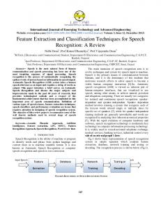
Fig. 4. Classification of the HYMAP dataset using the PFE.
(25)
(23)
(24)
(20)
(22)
(16)
(18)
2
(14)
7
1
(21)
(15)
6
3
4
(17)
5
13
8
(19)
9
11
10
12
Fig. 5. Class hierarchy obtained on the AVIRIS dataset: Each leaf node is labelled with the ID of the class it represents. Each internal node is identified with a specific number.
13 − Water 12 − Mud Flats 11 11 − Salt Marsh 10 10 − Cattail Marsh 9 9 − Spartina Marsh 8 8 − Graminoid Marsh 7 7 − Hardwood Swamp 6 6 − Broad Leaf 5 5 − Slash Pine 4 4 − Oak Hammock 3 3 − Palm Hammock 2 2 − Willow Swamp 1 1 − Scrub 0 0 − Unclassified 13 12
Fig. 6. Classification of the AVIRIS dataset using the PFE.
5
Concluding Remarks
The PFE technique used in conjunction with the BHC architecture results in a formidable and computationally inexpensive combination that not only provides high accuracy for land-cover classification based on hyperspectral data, but also extracts useful domain knowledge. It is already known that the peaks and valleys are due to the chemistry (absorption or reflection) of materials. Some remote sensing experts have started defining various vegetation indices, focused on issues like that fact that green plants reflect in the near IR and absorb in the red, so ratios and differences are used. The PFE method can be used in exploratory mode, particularly with complex materials, to define indices. We plan to pursue the design of soft sensors that can reduce data on-board, by simply aggregating the spectral responses within each segment of bands. We would also like to further study the sensitivity of the resulting features to changing atmospheric conditions, and are currently gathering data for the same. We suspect that PFE based features will indeed be quite insensitive, and if so, this will be the most compelling reason yet for adopting the PFE methodology to a wide range of settings for intelligent analysis of remote sensing data.
Acknowledgments This research was supported in part by the NASA EO -1 program, Grant NCC5-463, NSF grant ITR 0312471, the Terrestrial Sciences Program of the Army Research Office(DAAG55-98-1-0287) and the Texas Advanced Technology Research Program(CSRA-ATP-009). We thank Joe Morgan, Amy Neuenschander and Yangchi Chen for their help with data preparation and interpretation of results.
References 1. Kumar, S., Ghosh, J., Crawford, M.M.: Best-bases feature extraction algorithms for classification of hyperspectral data. IEEE Trans. Geoscience and Remote Sensing 39 (2001) 1368–79 2. Landgrebe, D.: Hyperspectral image data analysis as a high dimensional signal processing problem. Special Issue of the IEEE Signal Processing Magazine 19 (2002) 17–28 3. Friedman, J.H.: An overview of predictive learning and function approximation. In Cherkassky, V., Friedman, J., Wechsler, H., eds.: From Statistics to Neural Networks, Proc. NATO/ASI Workshop, Springer Verlag (1994) 1–61 4. Kumar, S., Ghosh, J., Crawford, M.M.: Hierarchical fusion of multiple classifiers for hyperspectral data analysis. Pattern Analysis and Applications, spl. Issue on Fusion of Multiple Classifiers 5 (2002) 210–220 5. Jia, X., Richards, J.: Segmented principal components transformation for efficient hyperspectral remote-sensing image display and classification. IEEE Transactions on Geoscience and Remote Sensing 37 (1999) 538–542
6. Lee, C., Landgrebe, D.A.: Decision boundary feature extraction for neural networks. IEEE Transactions on Neural Networks 8 (1997) 75–83 7. Lee, C., Landgrebe, D.: Feature extraction based on decision boundaries. IEEE Transactions on Pattern Analysis and Machine Intelligence 15 (1993) 388–400 8. Jia, X.: Classification techniques for hyperspectral remote sensing image data. PhD thesis, Univ. College, ADFA, University of New South Wales, Australia (1996) 9. A. Koski, M.J., Meriste, M.: Syntactic recognition of ecg signals by attributed finite automata. Pattern Recognition 28 (1995) 1927–1940 10. Vullings, H., Verhaegen, M., H.B., V.: ECG segmentation using time-warping. In: Proceedings of the 2nd International Symposium on Intelligent Data Analysis. (1997) 11. Shatkay, H., Zdonik, S.: Approximate queries and representations for large data sequences. In: Proceedings of the 12th IEEE International Conference on Data Engineering. (1996) 546–553 12. Duda, R.O., Hart, P.E., eds.: Pattern Classification and Scene Analysis. Wiley, New York (1973) 13. Li, C., Yu, P., Castelli, V.: MALM: A framework for mining sequence database at multipleabstraction levels. In: Proceedings of the 7th International Conference on Information and Knowledge Management. (1998) 267–272 14. Lavrenko, V., Schmill, M., Lawrie, D., Ogilvie, P., Jensen, D., Allan, J.: Mining of concurent text and time series. In: Proceedings of the 6th International Conference on Knowledge Discovery and Data Mining. (2000) 37–44 15. Keogh, E., Smyth, P.: A probabilistic approach to fast pattern matching in time series databases. In: Proceedings of the 3rd International Conference of Knowledge Discovery and Data Mining. (1997) 24–30 16. Keogh, E., Pazzani, M.: An enhanced representation of time series which allows fast and accurate classification, clustering and relevance feedback. In: Proceedings of the 4th International Conference of Knowledge Discovery and Data Mining. (1998) 239–241 17. Keogh, E., Pazzani, M.: Relevance feedback retrieval of time series data. In: Proceedings of the 22th Annual International ACM-SIGIR Conference on Research and Development in Information Retrieval. (1999) 183–190 18. Keogh, E., Chu, S., Hart, D., Pazzani, M.: An Online Algorithm for Segmenting Time Series. In: Proceedings of IEEE International Conference on Data Mining. (2001) 289–296. 19. Tumer, K., Ghosh, J.: Robust combining of disparate classifiers through order statistics. Pattern Analysis and Applications, spl. Issue on Fusion of Multiple Classifiers 5 (2002) 20. Morgan, J.T., Henneguelle, A., Crawford, M.M., Ghosh, J., Neuenschwander, A.: Adaptive feature spaces for land cover classification with limited ground truth”. In Roli, F., Kittler, J., eds.: Multiple Classifier Systems. LNCS Vol. 2364, Springer (2002) 189–200 21. Jain, A.K.: Advances in statistical pattern recognition. In Devijver, F.A., Kittler, J., eds.: Pattern Recognition Theory and Applications. Springer-Verlag (1986) 1–19 22. Kumar, S.: Modular learning through output space decomposition. PhD thesis, Dept. of ECE, Univ. of Texas at Austin, Dec. (2000) 23. Ustun, R.: Spectral/spatial classification and output-based fusion for multisensor remotely sensed imaged data. Master’s thesis, The University of Texas at Austin, Austin, TX (2000)