Classification Using Support Vector Machines with Graded Resolution Lipo Wang*t, Bing Liut and Chunru Want College of Information Engineering, Xiangtan University, Xiangtan, Hunan, China Email:
[email protected] t School of Electrical and Electronic Engineering, Nanyang Technology University, Block S1, 50 Nanyang Avenue, Singapore 639798
*
Abstract- A method which we call support vector machine with graded resolution (SVM-GR) is proposed in this paper. During the training of the SVM-GR, we first form data granules to train the SVM-GR and remove those data granules that are not support vectors. We then use the remaining training samples to train the SVM-GR. Compared with the traditional SVM, our SVM-GR algorithm requires fewer training samples and support vectors, hence the computational time and memory requirements for the SVM-GR are much smaller than those of a conventional SVM that use the entire dataset. Experiments on benchmark data sets show that the generalization performance of the SVM-GR is comparable to the traditional SVM. Keywords: granular support vector machine, granular computing I. INTRODUCTION
SVMs have shown great capabilities in solving various classification problems [1]-[6]. In many applications, SVMs have outperformed many other machine learning methods [1] and have established themselves as a powerful tool for classification problems. When performing a pattem recognition task, the SVM first maps the input data into a high-dimensional feature space and then finds an optimal separating hyperplane to maximizes the margin between two classes in this highdimensional space. Maximizing the margin is a quadratic programming (QP) problem and can be solved by using some optimization algorithms [7]. However, for large-scale training sets, two major problems still exist for standard SVMs with traditional optimization algorithms, such as Newton and Quasi-Newton [8]. First, most computation consumed in the support vector learning is to solve a full dense matrix Q, where Q E RW is a positive semi-definite matrix and 1 is the number of training samples. Therefore, the time complexity is exponential with respect to 1. [9], [10]. Second, solving the QP problem needs storing the matrix Q. Hence, the memory requirements will grow with square of the size of training sample, which may become too large for large data sets. [8] One major method to solve these problems is the decomposition method [11], which solves a sequence of smallersized QP problems so that the the memory and computation difficulties can be avoided. However, for huge problems with many support vectors, the training speed of the decomposition method is still very slow [8]. Recently, Lee and Mangasarian [9] proposed the reduced SVM (RSVM) to reduce the computation complexity. The key idea of the RSVM is to randomly select a subset of training data as candidates of 0-7803-9017-2/05/$20.00 02005 IEEE
support vectors and use the whole training set as constraints, in order to obtain a smaller QP problem. But in this method, the 'support vectors' are chosen randomly, which leads to the unstable results. Zheng et al. [10] extended the RSVM by applying unsupervised clustering methods to select candidates of support vectors. They stated that the modified RSVM algorithm achieves more stable results and higher classification accuracy in comparison to the RSVM. However, it should be noticed that many unsupervised clustering methods also have high time complexity. Therefore, the modified RSVM algorithm may also be slower than the RSVM and not suitable for large problems. In this paper, we propose a novel learning method called SVM with graded resolution (SVM-GR), which uses ideas in granular computing method to solve the QP problem. Granular computing is an emerging conceptual paradigm of computing with information granules [12] [13]. Information granules are collections of entities, usually originating at the numeric level, and then arranged together due to their similarity, functional adjacency, indistinguishability, coherency or alike [14]. There are a number of formal models of of information granules including interval analysis, fuzzy sets, rough sets, shadowed sets and probabilistic sets. Information granules are processed as follows [12]. Depending upon the problem, we usually group granules of similar "size" (or called granularity) together in a single layer. If more detailed processing is required, smaller information granules are sought and then these granules are arranged in another layer. Recently, granular computing has been successfully applied to many areas, such as data mining [15], image compression [16], signal analysis [17] and neural network design [18], [19]. In 2004, Tang et al. [20] proposed the GSVM algorithm that used the granular computing methods to build SVMs. In [20], the whole feature space was split into a set of subspaces and for each subspace a hyperplane was built. Training the GSVM required to maximize the margin width for each subspace simultaneously. The proposed SVM-GR method is inspired by the essential result in support vector learning, i.e., the optimal separating hyperplane is determined by only the support vectors. Since all the non-support-vector samples have no contribution to set up the optimal hyperplanes, we can filter these samples in advance and use the remaining data to perform support vector
666
learning. The development of the SVM-GR involves two main phases as follows: 1) Rough Filtering: Divide each input dimension into r equal segments. The input space thus forms r' data granules, where n is the dimensionality of the input space. Use the average within each granule to train a SVM. The non-support vector granules are filtered (ignored in further training). 2) Elaborate Learning: Release the training samples from the remaining support vector granules. These training samples are used for final support vector learning. 3) If the data set is very large, rather than using all data in the support vector granules for training the SVM directly in step 2, we can form smaller granules within these larger granules obtained in Step 1 and filter nonsupport-vector granules again. The number of levels in this hierarchical granulation may be as large as needed. Although support vector learning is carried out in all phases, the sizes of training datasets are much smaller than that of the whole training dataset and hence the time complexity can be reduced greatly. Experimental results show that, for a large-scale problem with up to tens of thousands of data, the size of training data in the SVM-GR algorithm is decreased to one tenth of the original size and hence the SVM-GR algorithm provides a much faster speed than the conventional SVMs. Experimental results also indicate that the SVM-GR algorithm produces a comparable generalization performance in comparison to the traditional SVMs. Although both the proposed SVM-GR and the GSVM are based on the granular computing concept, the training for these two algorithms are quite different. Different from our paper, there are no filtering process and final training process in [20]. Since all data have to be used simultaneously to train SVMs, the speed of the GSVM [20] cannot be very fast. Our paper is organized as follows. A brief review of the conventional theory will be described in Section 2. In Section 3, we propose the SVM-GR algorithm. Performance evaluation of the proposed SVM-GR is presented in Section 4. Finally, discussions and conclusions are given in Section 5. II. SVMs FOR CLASSIFICATION
Given .a training set (Xi, Yi), i = 1, 2, ..., 1, where xi E Rn and yi E {-1, 1}, the traditional SVM algorithm is summarized as the following optimization problem:
and transformed into dual
i=l j=l
i=l
subject to: Zaiyi =0 ; O < ai < C, for=i
1, 2, ...,1
i=l1
(2)
where K(xi, xj) = q(xi)Tq(xj) is the kernel function, a-= (a1,a2, ... al) is the vector of nonnegative Lagrange multipliers. Suppose the optimum values of the Lagrange multipliers are denoted as ao,i (i = 1, 2, ..., 1), we may determine the corresponding optimum value of the linear weight vector wo and the optimal hyperplane as in (3) and (4), respectively: I
wo
=
ao,iyiq(xi) E i=l
(3)
I
ZEo,iyiK(X xi) = 0
(4)
i=l
and the decision function is
f(x) = sign
a,,iyiK(xi, x) + b)
(5)
III. THE SVM-GR ALGORITHM A. Data Granules
We use the interval analysis to form the data granules [12]. An interval vector [bkl in Rn is defined as a Cartesian product of n intervals as follows:
[bkl = [bk,11 X [bk,2]
x
...
x
[bk,n],
k = 1, 2, ..., N
(6)
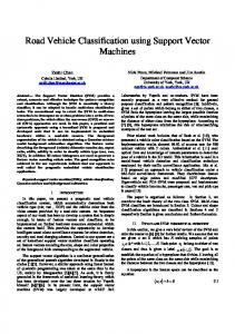
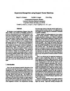
where bk,i are intervals, [bk,i] = [bkmi-n- bmax]. 1< i < n and n is the dimensionality of the input space. The interval vectors in Rf2 are showed in Figure 1. Assume X is a measurable compact subset of the n-dimensional Euclidean space Rn and all training data xi E X. X can be represented as the union of interval vectors, i.e., X = [b1] U [b2] U ... U [b1l], and [bk] n [bj] = q for any k 74 j, 1 < k,j < 11, where 11 is the total number of data granules. Then we define the data granules (ak, tk) as follows:
w,b,{ 2
subject to: yi (wTq(Xi) + b) > 1-
>1Ei ELst aiajyiyjK(xi, xj)
max Q(a) = Z a(i-
ak
(1)
tk
where +(x) is a nonlinear function that maps x into a higher dimensional space. w, b and (i are the weight vector, bias and slack variable, respectively. C is a constant and determined a priori. Searching the optimal hyperplane in (1) is a QP problem, which can be solved by constructing a Lagrangian
=
=
mean{xi Ixi c [bk]}
(7)
(I:
(8)
sign
Yi)
Xi C[bk]
In our SVM-GR algorithm, we assume the widths of all intervals are same, i.e., bk -j bkii = d, where d is the parameter to determine granularity of data. Assume all xi E 667
vector learning elaborately. We release the training samples from the support vector granules. These samples are used for finally support vector learning. Noticed that many training samples are filtered in the first step, hence the number of training samples for SVM in this phase is much smaller and [bpPI I= [bp+1 ] the computation can be reduced. If the dataset in the second step is still very large, we can form smaller granules within these large granules obtained in step 1 and filter non-support-vector granules again. The [bk ] [bk+l] number of levels in this hierarchical granulation may be as large as needed. In this way, we can assure that the k,2 dataset in each phase is not very large and hence the training d d computation and storage difficulties can be solved. The proposed SVM-GR algorithm can be summarized as follows: Algorithm 1: Given a training set 'po = {(xi,yi)lxi E Rnf yi E {-1, 1}, i = 1, 2, ...,1}, we conduct the following: Fig. 1. Interval vectors in R2. The widths of all intervals are same and equal 1) Normalize xi (i = 1, 2, ..., 1) to the range [dmin, dmax]n; to d. 2) Choose the interval vector [bk] as (9) and (10), then form the data granules (ak, tk) as (7) and (8). Non-empty data granules form the new training dataset defined as [dmin, dmax]n and dmax -dmin = r d, then the interval vector 'P1 = {(ak,tk)jak E [dmin,dmax]n, tk E {-1,1},k = [bk] is formed as follows: 1,2, ... 1111. out support vector learning using the dataset pj1. Carry 3) [b] =[dmin, dmin + d]n; vector granules form a set E. Then release The support [b2] = [dmin, dmin + 2d] x [dmin, dmin + d]n-1; the training samples from (E and form another training set defined as 'P2 = {(Xi Yi)Ixi E bk,ak E E3}. (9) [bk] = [dmin + Si d, dmin + (Si + 1) .d] x ... 4) If the size of 'P2 is smaller than Mo then turn to Step x [dmin + Sn di dmin + (Sn + 1) d]; 2, otherwise turn to Step 5. Here Mo is the maximum size of the training set that is determined a priori. Carry out support vector learning using the dataset 'P2 5) [b1l] = [dmax d, dmax]n, and predict the test set. where IV. EXPERIMENTAL RESULTS Sn = (k - 1) mod (rn-1) + 1; In this section, we conducted experiments on some comSn-1 = [(k - 1) - (Sn - 1)rn-1] mod rn-2 + 1; monly used problems. For the classification problems, we conduct experiments on three data sets from UCI database sm = ( - 1) - Ei=m+l (Si - 1) *ri-]mdrm1+1 [21] ( satimage, letter and shuttle ). The problem statistics are given in Table I. sl = [(k-1)-E2(s -1)ri-11 + 1, TABLE I (10) PROBLEM STATISTICS < where 1