Support Vector Machines for Pattern Classification

Support Vector Machines for Pattern Classification Shigeo Abe Graduate School of Science and Technology Kobe University Kobe, Japan

My Research History on NN, FS, and SVM • Neural Networks (1988-) – Convergence characteristics of Hopfield networks – Synthesis of multilayer neural networks

• Fuzzy Systems (1992-) – Trainable fuzzy classifiers – Fuzzy classifiers with ellipsoidal regions

• Support Vector Machines (1999-) – Characteristics of solutions – Multiclass problems

Contents Contents 1. Direct and Indirect Decision Functions 2. Architecture of SVMs 3. Characteristics of L1 and L2 SVMs 4. Multiclass SVMs 5. Training Methods 6. SVM-inspired Methods 6.1 Kernel-based Methods 6.2 Maximum Margin Fuzzy Classifiers 6.3 Maximum Margin Neural Networks

Multilayer Multilayer Neural Neural Networks Networks Neural networks are trained to output the target values for the given input. Class 1

N.N.

Class 1 1 0 Class 2

Class 2

Multilayer Multilayer Neural Neural Networks Networks Indirect decision functions: decision boundaries change as the initial weights are changed. Class 1

N.N.

Class 1 1 0 Class 2

Class 2

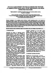
Support Support Vector Vector Machines Machines Direct decision functions: decision boundaries are determined to minimize the classification error of both training data and unknown data. Class 1

SVM

If D(x) > 0, Class 1 Otherwise, Class 2

Maximum margin Class 2

Optimal hyperplane (OHP) D(x) = 0

Summary Summary • When the number of training data is small, SVMs outperform conventional classifiers. • By maximizing margins performance of conventional classifiers can be improved.


Architecture Architecture of of SVMs SVMs • Formulated for two-class classification problems • Map the input space into the feature space • Determine the optimal hyperplane in the feature space

Class 2

g(x)

Class 1 OHP Input Space

Feature Space

Types Types of of SVMs SVMs • Hard margin SVMs – linearly separable in the feature space – maximize generalization ability

• Soft margin SVMs – Not separable in the feature space – minimize classification error and maximize generalization ability

Class 2 Class 1

• L1 soft margin SVMs (commonly used) • L2 soft margin SVMs

Feature Space

Hard Hard Margin Margin SVMs SVMs We determine OHP so that the generalization region is maximized:

Margin δ

Generalization region

maximize δ subject to wtg(xi ) + b ≧ 1 for Class 1 − wtg(xi ) − b ≧ 1 for Class 2

Class 1 yi = 1 Class 2 yi = − 1

+ side

Combining the two: yi (wtg( xi ) + b) ≧ 1

OHP D(x) = wtg(xi ) + b = 0

Hard Hard Margin Margin SVM SVM (2) (2) The distance from x to OHP is given by yi D(x) /||w||. Thus all the training data must satisfy

Margin δ

yi D(x) /||w|| ≧ δ . Imposing ||w|| δ = 1, the problem is to minimize ||w||2/2 subject to yi D(xi) ≧ 1

for i = 1,…,M.

Generalization region

Class 1 yi = 1 Class 2 yi = − 1

+ side

OHP D(x) = wtg(xi ) + b = 0

Soft Soft Margin Margin SVMs SVMs If the problem is nonseparable, we introduce slack variables ξi. Minimize ||w||2/2 + C/p Σi=1,M ξip subject to yi D(xi) ≧ 1 − ξi where C: margin parameter, p = 1: L1 SVM, = 2: L2 SVM

Margin δ

Class 1 yi = 1

1> ξi > 0 Class 2 yi = − 1

ξk >1 + side

OHP D(x) = 0

Conversion Conversion to to Dual Dual Problems Problems Introducing the Lagrange multiplies αi and βi, Q = ||w||2/2 +C/p Σi ξip −Σi αi(yi(wtg(xi) + b) −1+ξi) [−Σ −Σi βiξi ] The Karush-Kuhn-Tacker (KKT) optimality conditions: ∂Q/∂ ∂w = 0,∂ ∂Q/∂ ∂b = 0,∂ ∂Q/∂ ∂ξi = 0, αi > 0, βi > 0 KKT complementarity conditions αi(yi(wtg(xi) + b) −1+ξi) = 0, [(βiξi = 0 ]. When p = 2, terms in [ ] are not necessary.

Dual Dual Problems Problems of of SVMs SVMs L1 SVM Maximize 　　Σ 　　Σi αi − C/2 Σi,j αi αj yi yj g(xi )tg(xj) subject to 　　Σ 　　Σi yi αi = 0, C ≧ αi ≧0. L2 SVM Maximize 　　Σ 　　Σi αi − C/2 Σi,j αi αj yi yj (g(xi )tg(xj) + δij /C) subject to 　　Σ 　　Σi yi αi = 0, αi ≧0, where δij : 1 for i = j and 0 for i ≠ j.

KKT KKT Complementarity Complementarity Condition Condition For L1 SVMs, from αi(yi(wtg(xi) + b) −1+ξi) = 0, − αi) ξi = 0, there are three cases for αi : βiξi = (C− 1. αi = 0. Then ξi = 0. Thus xi is correctly classified, 2. 0 < αi < C. Then ξi = 0, and wtg(xi) + b = yi, 3. αi = C. Then ξi ≧ 0. Training data xi with αi > 0 are called support vectors and those with αi = C are called bounded support vectors. The resulting decision function is given by D(x) = Σi αiyig(xi)t g(x) + b.

Kernel Kernel Trick Trick Since mapping function g(x) appears in the form of g(x)tg(x’), we can avoid treating the variables in the feature space by introducing the kernel: H(x,x’) = g(x)tg(x’). The following kernels are commonly used: 1. Dot product kernels: H(x,x’) = xtx’ 2. Polynomial kernels: H(x,x’) = (xtx’+1)d 3. RBF kernels : H(x,x’) = exp(− − γ ||x − x’||2)

Summary Summary • The global optimum solution by quadratic programming (no local minima). • Robust classification for outliers is possible by proper value selection of C. • Adaptable to problems by proper selection of kernels.


Hessian Hessian Matrix Matrix Substituting αs = - ysΣyi αi into the objective function, Q = αt 1 - 1/2 αt H α we derive the Hessian matrix. L1 SVM HL1 = (… yi (g(xi) − g(xs) ) …)t(… yi (g(xi) − g(xs) ) …) HL1: positive semidefinite L2 SVM HL2 = HL1 + {(yi yj + δij)/C} HL2: positive definite, which results in stabler training.

Non-unique Non-unique Solutions Solutions Strictly convex functions give unique solutions.

Table Uniqueness Primal Dual

L1 SVM L2 SVM Non-unique* Unique* Non-unique Unique*

*: Burges and Crisp (2000) Convex objective function

Property Property 11 For the L1 SVM, the vectors that satisfy yi(wtg(xi) + b) = 1 are not always support vectors. We call these boundary vectors.

1 3 2

Irreducible Irreducible Set Set of of Support Support Vectors Vectors A set of support vectors is irreducible if deletion of boundary vectors and any support vectors result in the change of the optimal hyperplane.

Property Property 22 For the L1 SVM, let all the support vectors be unbounded. Then the Hessian matrix associated with the irreducible set is positive definite.

Property Property 33 For the L1 SVM, if there is only one irreducible set, and support vectors are all unbounded, the solution is unique.

Irreducible sets {1, 3}, {2, 4}

2 1 4 3

The dual problem is non-unique, but the primal problem is unique.

In general the number of support vectors of L2 SVM is larger than that of L1 SVM.

Computer Computer Simulation Simulation • We used white blood cell data with 13 inputs and 2 classes, each class having app. 400 data for training and testing. • We trained SVMs using the steepest ascent method (Abe et al. (2002)) • We used a personal computer (Athlon 1.6Ghz) for training.

Recognition Recognition Rates Rates for for Polynomial Polynomial Kernels Kernels The difference is small. 100 95 L1 L2 L1 L2

% 90 85 80 75

dot

poly2

poly3

poly4

poly5

Test Test Train. Train.

Support Support Vectors Vectors for for Polynomial Polynomial Kernels Kernels For poly4 and poly5 the numbers are the same. 200 180 160 140 120 100 80 60 40 20 0

L1 L2

dot

poly2

poly3

poly4

poly5

Training Training Time Time Comparison Comparison As the polynomial degree increases, the difference becomes smaller. 60 50 40

(s)

L1 SVM L2 SVM

30 20 10 0

dot

poly2

poly3

poly4

poly5

Summary Summary • The Hessian matrix of an L1 SVM is positive semi-definite, but that of an L2 SVM is always positive definite. • Thus dual solutions of an L1 SVM are nonunique. • When non-critical the difference between L1 and L2 SVMs is small.


Multiclass Multiclass SVMs SVMs • One-against-all SVMs – Continuous decision functions – Fuzzy SVMs – Decision-tree-based SVMs

• Pairwise SVMs – Decision-tree-based SVMs (DDAGs, ADAGs) – Fuzzy SVMs

• ECOC SVMs • All-at-once SVMs

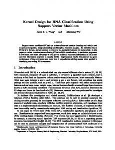
One-against-all One-against-all SVMs SVMs Determine the ith decision function Di(x) so that class i is separated from the remaining classes. Classify x into the class with Di(x) > 0. D3(x) = 0 Class 2

Class 2 D2(x) = 0

Class 1

Class 3

Class 1

Class 3

D1(x) = 0

Unclassifiable

Continuous Continuous SVMs SVMs Classify x into the class with max Di(x). 0 > D2(x) > D3(x) 0 > D2(x) > D1(x)

D2(x) > D3(x) D3(x) = 0

Class 2

Class 2

D2(x) = 0

Class 1

Class 3 Class 1 D1(x) = 0

Class 3

Fuzzy Fuzzy SVMs SVMs D1(x) = 1 D1(x) = 0

Class 1

Class 2

Class 3

m11(x)

1 0

Membership function

We define a onedimensional membership function in the direction orthogonal to the decision function Dij(x).

Class Class ii Membership Membership Class i membership function m1(x) = 0.5

mi ( x) = min mij ( x). j =1,..., n

The region that satisfies mi(x) > 0 corresponds to the classifiable region for class i.

m1(x) =1

Class 1

m1(x) = 0

Resulting Resulting Class Class Boundaries Boundaries by by Fuzzy Fuzzy SVMs SVMs The generalization regions are the same with those by continuous SVMs.

Class 2

Class 2

Class 1

Class 3

Class 1

Class 3

Decision-tree-based Decision-tree-basedSVMs SVMs Each node corresponds to the hyperplane. Training step

Classification step

At each node, determine Starting from the top node, calculate the value until a OHP. leaf node is reached. Class i

f i (x ) = 0

f i (x )

-

+ Class k Classj f j (x ) = 0

f j (x )

Classi + Classj

Class k

The The problem problem of of the the decision decision tree tree • Unclassifiable region can be resolved. • The region of each class depends on the structure of a decision tree. Class i

f i (x ) = 0

Class k

Class i f j(x ) = 0

Class j

Class j f j (x ) = 0

Class k f k (x ) = 0

How do we determine the decision tree?

Determination Determination of of the the decision decision tree tree ?

The overall classification performance becomes worse.

The separable classes need to be separated at the upper node. The separability measures: Euclidean distances between class centers Classification errors by the Mahalanobis distance z z

1 vs. remaining classes Some vs. remaining classes

11 Class Class vs. vs. Remaining Remaining Classes Classes Using Using Distances Distances between between Class Class Centers Centers Class

Separate the farthest class from remaining classes.

i Class

f i (x ) = 0

f l (x ) = 0 Class

j Class

f j (x ) = 0

l

k

Calculate distances between class centers. For each class, find the smallest value. Separate the class with the largest value in step 2. Repeat for remaining classes.

Pairwise Pairwise SVMs SVMs For all pairs of classes i, j, we define n(n-1)/2 decision functions and classify x into class arg maxi Di(x) where Di(x) = Σjsign Dij(x) D12 (x) = 0 Class 1 D31(x) = 0

Class 2 Class 3 D23(x) = 0

Unclassifiable regions still exist. D1(x) = D2(x) = D3(x) = 1

Pairwise Pairwise Fuzzy Fuzzy SVMs SVMs The generalization ability of the P-FSVM is better than the P-SVM.

Class 1

Class 1 class 2

Class 3

P-SVM

Class 2 Class 3

P-FSVM

Decision-tree-based Decision-tree-based SVMs SVMs (DDAGs) (DDAGs) Generalization regions change according to the tree structure. D12(x) 2

1

D13(x) 3

Class 1

Class 1

D32(x) 1

2

Class 3

3

Class 2

class 2 Class 3

Decision-tree-based Decision-tree-based SVMs SVMs (ADAGs) (ADAGs) For three-class problems ADAGs and DDAGs are equivalent. In general, DDAGs include ADAGs.

1

2

D12(x)

3

2

1

D13(x) 3

ADAG (Tennis Tournament)

Class 1

D32(x) 1

2

Class 3

3

Class 2

Equivalent DDAG

ECC ECC Capability Capability The maximum number of decision functions = 2n-1 -1, where n is the number of classes. Error correcting capability = (h-1)/2, where h is the Hamming distance. For n = 4, h = 4 and ecc of 1. Class 1 1 1 1 -1 1 1 Class 2 1 1 -1 1 1 -1 Class 3 1 -1 1 1 -1 1 Class 4 -1 1 1 1 -1 -1

-1 1 1 -1

Continuous Continuous Hamming Hamming Distance Distance Di(x) = 1

Hamming Distance

Di(x) = 0

= Σ ERi(x) Class k

Class l

1 0

Error function

= Σ(1 − mi(x)) Equivalent to membership functions with sum operators Membership function

All-at-once All-at-once SVMs SVMs Decision functions wi g(x) + bi > wjg(x) + bj for j ≠ i, j=1,…,n Original formulation n ×M variables where n: number of classes M: number of training data Crammer and Singer (2000) ’s M variables

Performance Performance Evaluation Evaluation • Compare recognition rates of test data for one-against-all and pairwise SVMs. • Data sets used: – – – –

white blood cell data thyroid data hiragana data with 50 inputs hiragana data with 13 inputs 水戸57 水戸ひ

５９－１６

Japanese License Plate

Data Data Sets Sets Used Used for for Evaluation Evaluation Data

Inputs

Classes

Train.

Test

Blood Cell

13

12

3097

3100

Thyroid

21

3

3772

3428

H-50

50

39

4610

4610

H-13

13

38

8375

8356

Performance Performance Improvement Improvement for for 1-all 1-all SVMs SVMs SVM

FSVM

Tree

100 98 96 (%) 94 92 90 88 86 84 82

Performance improves by fuzzy SVMs and decision trees.

Blood

Thyroid

H-50

Performance Performance Improvement Improvement for for Pairwise Pairwise Classification Classification SVM ADAG MX ADAV MN

FSVM ADAG Av

100 98

(%) 96

FSVMs are comparable with ADAG MX.

94 92 90 88 86

Blood

Thyroid

H-13

Summary Summary • One-against-all SVMs with continuous decision functions are equivalent to 1-all fuzzy SVMs. • Performance of pairwise fuzzy SVMs is comparable to that of ADAGs with maximum recognition rates. • There is no so much difference between oneagainst-all and pairwise SVMs.


Research Research Status Status • Too slow to train by quadratic programming for a large number of training data. • Several training methods have been developed: – decomposition technique by Osuna (1997) – Kernel-Adatron by Friess et al. (1998) – SMO (Sequential Minimum Optimization) by Platt (1999) – Steepest Ascent Training by Abe et al. (2002)

Decomposition Decomposition Technique Technique Decompose the index set into two: B and N. Maximize 　　Q( 　　 α) = Σi∈ ∈B αi − C/2 Σi,j∈ ∈B αi αj yi yj H(xi, xj) − C Σi∈ ∈B, j∈ ∈N αi αj yi yj H(xi, xj) − C/2 Σi,j∈ ∈N αi αj yi yj H(xi, xj) + Σi∈ ∈N αi subject to 　　Σ 　　Σi∈ ∈B yi αi = − Σi∈ ∈N yi αi , C ≧ αi ≧0 for i ∈Β fixing αi for i ∈Ν.

Solution Solution Framework Framework

Outer Loop Inner Loop

Use of QP Package e.g., LOQO (1998)

Violation of KKT Cond Solve for working Set {αi | i ∈ B}

Fixed Set {αi | i ∈ N}

αi = 0

Solution Solution without without Using Using QP QP Package Package • SMO – |B| = 2, i.e., solve the problem for two variables – The subproblem is solvable without matrix calculations

• Steepest Ascent Training – Speedup SMO by solving subproblems with variables more than two

Solution Solution Framework Framework for for Steepest Steepest Ascent Ascent Training Training Outer Loop

Inner Loop Update αi for i ∈ B’ until all αi in B are updated.

Violation of KKT Cond

Working Set {αi | i ∈ B’} B’ ⊇B

Fixed Set {αi | i ∈ N}

αi = 0

Solution Solution Procedure Procedure • Set the index set B. • Select αs and eliminate the equality constraint by substituting αs = − ysΣ yj αj into the objective function. • Calculate corrections by ∂2Q/∂ ∂α2B”)−1 ∂Q/∂ ∂αB” αB” = −(∂ where B” = B’ -{s}. • Correct variables if possible.

Calculation Calculation of of corrections corrections • We calculate corrections by the Cholesky decomposition. • For the L2 SVM, since the Hessian matrix is positive definite, it is regular. • For the L1 SVM, since the Hessian matrix is positive semi-definite, it may be singular.

= Dii

If Dii < η, we discard the variables αj, j≧ i.

Update Update of of Variables Variables

1 2 3

• Case 1 Variables are updated. • Case 2 Corrections are reduced to satisfy constraints. • Case 3 Variables are not corrected.

Performance Performance Evaluation Evaluation • Compare training time by the steepest ascent method, SMO, and the interior point method. • Data sets used: – – – –

white blood cell data thyroid data hiragana data with 50 inputs hiragana data with 13 inputs 水戸57 水戸ひ

５９－１６

Japanese License Plate


Inputs

Classes

Train.

Test

Blood Cell

13

12

3097

3100

Thyroid

21

3

3772

3428

H-50

50

39

4610

4610

H-13

13

38

8375

8356

Effect Effect of of Working Working Set Set Size Size for for Blood Blood Cell Cell Data Data L1 SVM

L2 SVM

1200 1000

(s)

Dot product kernels are used.

800 600

For a larger size, L2 SVMs are trained faster.

400 200 0

2

4

13

20

30

Effect Effect of of Working Working Set Set Size Size for for Blood Blood Cell Cell Data Data (Cond.) (Cond.) L1 SVM

L2 SVM

700 600

Polynomial kernels with degree 4 are used.

500

(s) 400 300

No much difference for L1 and L2 SVMs.

200 100 0

2

20

40

Training Training Time Time Comparison Comparison LOQO

SMO

SAM

10000 1000

LOQO: LOQO is combined with decomposition technique.

(s) 100 10 1

Thyroid Blood H-50 H-13

SMO is the slowest. LOQO and SAM are comparable for hiragana data.

Summary Summary • The steepest ascent method is faster than SMO and comparable for some cases with the interiorpoint method combined with decomposition technique. • For the critical cases, L2 SVMs are trained faster than L1 SVMs, but for normal cases they are almost the same.


SVM-inspired SVM-inspired Methods Methods • Kernel-based Methods – – – –

Kernel Perceptron Kernel Least Squares Kernel Mahalanobis Distance Kernel Principal Component Analysis

• Maximum Margin Classifiers – Fuzzy Classifiers – Neural Networks


Fuzzy Fuzzy Classifier Classifier with with Ellipsoidal Ellipsoidal Regions Regions Membership function mi(x) = exp(- hi2(x)) hi2(x) = di2(x)/αi di2(x) = (x – ci)t Qi-1 (x – ci) where αi: a tuning parameter, di2(x): a Mahalanobis distance.

Training Training

1. For each class calculate the center and the covariance matrix. 2. Tune the membership function so that misclassification is resolved.

Comparison Comparison of of Fuzzy Fuzzy Classifiers Classifiers with with Support Support Vector Vector Machines Machines • Training of fuzzy classifiers is faster than support vector machines. • Comparable performance for the overlapping classes. • Inferior performance when data are scarce since the covariance matrix Qi becomes singular.

Improvement Improvement of of Generalization Generalization Ability Ability When When Data Data Are Are Scarce Scarce • by Symmetric Cholesky factorization, • by maximizing margins.

Symmetric Symmetric Cholesky Cholesky Factorization Factorization In factorizing Qi into two triangular matrices: Q i = L i L it, if the diagonal element laa is laa < η namely, Qi is singular, we set laa = η.

laa

Concept Concept of of Maximizing Maximizing Margins Margins

If there are no overlap between classes, we set the boundary at the middle of two classes, by tuning αi.

Upper Upper Bound Bound of of ααii The class i datum remains correctly classified for the increase of αi. We calculate the upper bound for all the class i data.

Lower Lower Bound Bound of of ααii The class j datum remains correctly classified for the decrease of αi. We calculate the lower bound for all the data not belonging to class i.

Tuning Tuning Procedure Procedure 1. Calculate the upper bound Li and lower bound Ui of α i. 2. Set αi = (Li + Ui)/2. 3. Iterate the above procedure for all the classes.

Data Data Sets Sets Used Used for for Evaluation Evaluation Data Inputs Classes Train. Test H-50

50

39

4610

4610

H-105

105

38

8375

8356

H-13

13

38

8375

8356

Recognition Rate of Hiragana-50 Data (Cholesky Factorization) Test 100 90 80 70 60 (%) 50 40 30 20 10 0

Train.

The recognition rate improved as η was increased.

10-5 10-4 10-3 10-2 10-1 η

Recognition Rate of Hiragana-50 Data (Maximizing Margins) Test

Train.

100 98

The better recognition rate for small η.

96

(%) 94 92 90 88 86 84

10-5 10-4

10-3 10-2 10-1 η

Performance Comparison CF 100 99 98 97 (%) 96 95 94 93 92 91

CF+MM

SVD

SVM

Performance excluding SVD is comparable.

H-50

H-105

H-13

Summary Summary • When the number of training data is small, the generalization ability of the fuzzy classifier with ellipsoidal regions is improved by – the Cholesky factorization with singular avoidance, – tuning membership functions when there is no overlap between classes.

• Simulation results show the improvement of the generalization ability.


Maximum Maximum Margin Margin Neural Neural Networks Networks • Training of multilayer neural networks (NNs) • Back propagation algorithm (BP) - Slow training

• Support vector machine (SVM) with sigmoid kernels - High generalization ability by maximizing margins - Restriction to parameter values

• CARVE Algorithm(Young & Downs 1998) - Efficient training method not developed yet

CARVE CARVE Algorithm Algorithm • A constructive method of training NNs • Any pattern classification problems can be synthesized in 3-layers (input layer included) • Needs to find hyperplanes that separate data of one class from the others

CARVE CARVE Algorithm Algorithm (hidden (hidden layer) layer) : The class for separation • Only

x2

x1

data are separated

Input space

x1 x2

The weights between input layer and hidden layer represent the hyperplane

Bias Input layer Hidden layer

CARVE CARVE Algorithm Algorithm (hidden (hidden layer) layer) : The class for separation x2

x1

Input space

x1 x2

• Only data are separated • Separated data are not used in next training • When only data of one class remain, the hidden layer training is finished

The weights between input layer and hidden layer represent the hyperplane

Bias Input layer Hidden layer

CARVE CARVE Algorithm Algorithm (output (output layer) layer) (0,1,0) Sigmoid function

(0,0,0)

(0,0,1)

(0,0,1)

1

(1,1,0) (1,0,0)

0

Input space

(0,0,0)

(1,0,0)

Hidden layer output space

All data can be linearly separable by the output layer

Proposed Proposed Method Method • NN training based on CARVE algorithm • Maximizing margins at each layer Optimal hyperplane

• On the positive side, data of other

classes may exist by SVM training

Input space

Not appropriate hyperplanes for CARVE algorithm

Extend DirectSVM method in hidden layer training and use conventional SVM training in output layer

Extension Extension of of DirectSVM DirectSVM • The class labels are set so that the class for separation are +1, and other classes are -1

Nearest data

Largest violation

ex.

target values

: +1 : ‐1

• Determine the initial hyperplane by DirectSVM method Input space

• Check the violation of the data with label –1

Extension Extension of of DirectSVM DirectSVM

Nearest data

• Update the hyperplane so that the misclassified datum with -1 is classified correctly Largest violation

Input space

If there are no violating data with label –1, we stop updating the hyperplane

Training Training of of output output layer layer • Apply conventional SVM training Maximum margin

Set weights by SVM with dot product kernels

x1 x2 Bias Input layer Bias

Hidden layer output space

Hidden layer

Output layer


Inputs

Classes

Train.

Test

Blood Cell

13

12

3097

3100

Thyroid

21

3

3772

3428

H-50

50

39

4610

4610

H-13

13

38

8375

8356

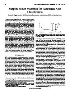
Performance Performance Comparison Comparison BP

FSVM

MM-NN

100

FSVM: 1 vs. all

98 96

(%)

MM-NN is better than BP and comparable to FSVMs.

94 92 90 88 86

Blood

Thyroid

H-50

Summary Summary • NNs are generated layer by layer by the CARVE algorithm and by maximizing margins. • Generalization ability is better than that of BP NN and comparable to that of SVMs.