Road Vehicle Classification using Support Vector Machines Zezhi Chen
Nick Pears, Michael Freeman and Jim Austin
Cybula Limited, York, UK
[email protected]
Department of Computer Science University of York, York, UK
[email protected],
[email protected]
Abstract— The Support Vector Machine (SVM) provides a robust, accurate and effective technique for pattern recognition and classification. Although the SVM is essentially a binary classifier, it can be adopted to handle multi-class classification tasks. The conventional way to extent the SVM to multi-class scenarios is to decompose an m-class problem into a series of twoclass problems, for which either the one-vs-one (OVO) or one-vsall (OVA) approaches are used. In this paper, a practical and systematic approach using a kernelised SVM is proposed and developed such that it can be implemented in embedded hardware within a road-side camera. The foreground segmentation of the vehicle is obtained using a Gaussian mixture model background subtraction algorithm. The feature vector describing the foreground (vehicle) silhouette encodes size, aspect ratio, width, solidity in order to classify vehicle type (car, van, HGV), In addition 3D colour histograms are used to generate a feature vector encoding vehicle color. The good recognition rates achieved in the our experiments indicate that our approach is well suited for pragmatic embedded vehicle classification applications. Keywords-support vector machine(SVM); vehicle classification; Gaussian mixture model;background subtraction
I.
INTRODUCTION
In this paper, we present a pragmatic road vehicle classification system, which automatically determines both vehicle type (car, van , HGV) and the vehicle color from the video stream provided by a road-side camera. An important aspect of our work has been to develop a system that is simple enough, in terms of feature vectors and classifiers, to be implemented on limited hardware resources embedded within the camera itself. This provides the opportunity to develop intelligent stand-alone surveillance systems for crime detection, security and road charging schemes. Central to our system are a set of kernelised support vector machine classifiers operating on feature vectors encoding the size, shape and color properties of the foreground blob corresponding to the segmented vehicle. The support vector algorithm is a nonlinear generalization of the generalized portrait algorithm developed in Russia in the sixties [1][2]. However, a similar approach using linear instead of quadratic programming was taken at the same time in the US, mainly by Mangasarian [3][4][5]. As such, it is firmly grounded in the framework of statistical learning theory, which has been developed over the last three decades by Vapnik himself [6][7][8]. In its present form, the support vector machine (SVM) was largely developed at AT&T Bell
Laboratories by Vapnik and co-workers. SVM have been recently proposed as a very effective method for general purpose classification and pattern recognition [8]. Intuitively, given a set of points which belong to either of two classes, a SVM finds the hyperplane leaving the largest possible fraction of points of the same class on the same side, while maximizing the distance of either class from the hyperplane. According to [7] [9], this hyperplane minimizes the risk of misclassifying examples of the test set. Prior related work includes that of Baek et al. [10], who presented a vehicle color classification based on the SVM. The implementation results showed 94.92 of success rate for 500 outdoor vehicle with 5 colors. Ambardekar et al. [11] used optical flow and knowledge of camera parameters to detect the pose of a vehicle in the 3D world. This information is used in a model-based vehicle detection and classification technique employed by their traffic surveillance application. Ma et al. [12] proposed an approach to vehicle classification under a mid-field surveillance framework. They discriminate feature based on edge points and modified SIFT descriptors. Eigenvehicle and PCA-SVM were proposed and implemented to classify vehicle into trucks, passenger cars, van and pick-ups in paper [13] The paper is organised as follows: In Section 2, we overview the basic theory of the two class SVM. Multi-class SVM classifiers are introduced in Section 3. Colour and shape classification algorithms are described in Sections 4 and 5 respectively Section 6 gives conclusions and further discussion. II.
TWO CLASS SVM: THEORETICAL OVERVIEW
In this section, we give a very brief review of the SVM and refer the reader to [8] [9] for further details. We assume that we are given a set S which has N training samples of points xi ∈ R m with i=1,2,…, N. Each point xi belong to either of two classes and thus is given a label yi ∈ {− 1,1} . The goal is to establish the equation of a hyperplane that divides S leaving all the points of the same class on the same side while maximizing the distance between the two classes and the hyperplane [12]. A hyperplane in the feature space can be described as the equation w, x + b = 0
(1)
where w ∈ R m and b is a scalar. When the training samples are linearly separable, SVM yields the optimal hyperplane that separates two classes with no training errors, and maximises the minimum distance from the training samples to the hyperplane. There is some redundancy in Eq. (1), and without loss of generality it is appropriate to consider a canonical hyperplane [7], where the parameters w, b are constrained by
min i w, xi + b = 1
(2)
This incisive constraint on the parameterisation is preferable to alternatives in simplifying the formulation of the problem. It states that the norm of the weight vector should be equal to the inverse of the distance of nearest point in the data set to the hyperplane. A separating hyperplane in the canonical form must satisfy the following constraints: yi [ w, xi + b] ≥ 1 , i = 1, 2, L , N
(3)
The optimal hyperplane is given by maximizing the margin ρ , subject to the constraints of Eq. (3). The margin is given by: ρ (w, b ) =
(
)
1 2 min xi , yi =1 w, xi + b + min xi , yi =−1 w, xi + b = w w
(4)
2
Since w is convex, minimizing it under linear constraints (3) can be achieved with Lagrange multipliers. If we denote by α = (α1 , α 2 , L , α N ) the N non negative Lagrange multipliers associates with constraints (3), the solution to the optimisation problem of Eq.(4) under the constraint Eq.(3) is given by the saddle point of the Lagrange function (lagrangian)
φ (w, b, α ) =
1 2 N w − ∑i =1 α i ( yi [ w, xi + b ] − 1) 2
(5)
Eq. (5) to be transform to its dual problem, which is easier to solve. The dual problem is given, 1 N N N max α w(α ) = max α ∑i =1 α i − ∑i =1 ∑ j =1 α i α j y i y j x i , x j (6) 2
Subject to,
α i ≥ 0 , i = 1,2, L , N ,
∑
N
i =1
α i yi = 0
This can be achieved by the use of standard quadratic programming method [15]. Once the vector * * * * α = α1 , α 2 , L , α N solution of the maximization problem (6) has been found, the optimal separating hyperplane is given by,
(
)
w* = ∑i =1 α i* yi xi N
b* = −
1 * w , xr + x s 2
(7) (8)
xr and xs are any support vector from each class satisfying, α r , α s > 0 and y r = −1 , y s = 1 . where
The hard classifier is then
(
f ( x ) = sign w* , x + b *
)
(9)
So far the discussion has been restricted to the case where the training data is linearly separable. However, in general this will not be the case. When the data is not linearly separable, there are two approaches to generalising the problem, which are dependent upon prior knowledge of the problem and an estimate of the noise on the data. In the case where it is expected (or possible even known) that a hyperplane can correctly separated the data, a methods of introducing an additional cost function associated with misclassification is appropriate. More generally, slack variable ξ = (ξ1 , ξ 2 , L , ξ N ) , with ξ i ≥ 0 was introduced in [8], such that
yi [ w, xi + b] ≥ 1 − ξ i , i = 1,2, L , N
(10)
to allow the possibility of examples that violate (3). The ξ i are a measure of the misclassification errors. The generalised optimal separating hyperplane is determined by the vector w that minimise the function
φ (w, ξ ) =
1 2 N w + C ∑i =1 ξ i 2
(11)
purpose of the first term is minimized to control the learning capacity as in the separable case; the second term is to control the number of misclassified points. The parameter C is chosen by the user, a larger C corresponding to assigning a higher penalty to errors. The only difference is that α i have upper bound C here. SVM training requires to fix C, the penalty term for misclassifications. So C must be chosen to reflect the knowledge of the noise on the data. For the applications where linear SVM does not produce satisfactory performance, nonlinear SVM is suggested. The basic idea is to map x by nonlinearly mapping φ (x ) to a much higher dimensional feature space, and by working with linear classification in that space in which the optimal hyperplane is found. The nonlinear mapping can be implicitly defined by introducing the so called kernel function K (xi , x j ) which computes the inner product of vectors φ ( xi ) and φ (x j ) . If we have K (xi , x j ) = φ (xi ) ⋅ φ (x j ) , then only K is needed in the
training algorithm and the mapping
φ
is never explicitly used.
From Mercer’s theory [16] [17], we know that given a symmetric positive kernel K ( x, y ) , exists a mapping φ such that K ( x, y ) = φ (x )φ ( y ) , as long as satisfies Mercer’s condition. Under the feature mapping, the solution of a SVM has the form:
(
f ( x ) = sign wˆ , φ ( x ) + bˆ
)
where
wˆ = ∑i =1 α i* yiφ ( xi ) N
1 bˆ = − wˆ , φ ( xr ) + φ ( xs ) 2
(13)
More convenient formula to determine the sign is f (x ) = sign
(
(∑
N
α i* yiφ ( xi ),φ (x ) + bˆ
i =1
= sign ∑i =1α y K ( xi , x ) + bˆ N
* i i
)
IV.
(12)
)
(14)
COLOUR CLASSIFICATION
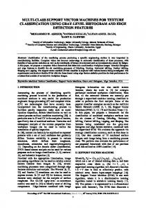
Four different colour (green, red, blue, yellow) objects images were selected from COIL (Columbia Object Image Library) database [14] to test our colour classification algorithm. The COIL images are colour images (24 bits for each of the RGB channels) of 128x128 pixels. The images consist of 7200images of 100 objects (72 views for each of the objects). The images were downloaded via anonymous ftp from the site www.cs.columbia.edu. As explained in detail in [27], the objects are positioned in the center of a turntable and observed from a fixed viewpoint. Figure 1 shows a selection of the object samples in the database.
where bˆ = − 1 N α * y [K (x , x ) + K (x , x )]. ∑i=1 i i i r i s 2
III.
THE MULTI-CLASS SVM CLASSIFIER
The solution of binary classification problems using SVMs is well developed. Multi-class problems (such as object recognition and image classification [18]) have typically been solved by combining independently produced binary classifiers. In the one-vs-all (OVA, or one-vs-rest) method, one constructs k classifiers, one for each class. The mth classifier constructs a hyperplane between class m and the k-1 other classes. If say the classes of interest in an image include car, HGV and van, classification would be effected by classifying car against non-car (i.e. HGV and van) or HGV against non-HGV (i.e. car and van). This method has been used widely in the support vector literature to solve multi-class pattern recognition problems [19][20][21]. Alternatively, onevs-one (OVO, or all-vs-all) approach involves constructing a machine for each pair of classes resulting in k (k − 1) 2 machines. For each distinct pairs m1 and m2 , we run the learning algorithm on a binary problem in which examples labelled y= m1 are considered positive, and those labelled y= m 2 are negative. All other examples are simply ignored. When applied to a test point, each classification gives one vote to the winning class and the point is labelled with the class having most votes. This approach can be further modified to give weighting to the voting process. Rifkin and Klautau [22] gave an extensive theoretical-based analysis, comparison about multiple classifications, such as OVA, OVO, RLSC (regularized least squares classification), COM (complete code) and ECOC (error correcting output coding). They indicated that OVA scheme is extremely powerful, producing results are often at least as accurate as other approaches. Anthony et al. [23] gave the similar conclusion that is the resulting classification accuracy of OVA is not significantly different from OVO approach. However, some researchers have different opinion. They reported that OVO scheme has a simple conceptual justification, and can be implemented to train faster and better performance than the OVA scheme although OVO are training O(k 2 ) classifiers rather than O(k ) for OVA scheme (the reason is the individual classifiers are much smaller, and given the time required to train on the point is generally superlinear), and the OVO scheme offers better performance that the OVA scheme [24][25][26].
Figure 1. Sample images in the COIL database.
Colour histogram technique is a vey simple and low-level method. Since we are dealing with discretely sampled data from colour images, we use discrete densities stored as m-bin histograms. In a discrete space, xi , i = 1, 2, · · · , n are the pixel locations of the model. A function b : R 2 → {1,2, L , m} associates to the pixel at location xi the index b( xi ) of the histogram bin corresponding to the value of that pixel. Hence a normalized histogram of the region of interest can be formed (using q as an example) q (u ) =
where
1 n ∑ δ [b( xi ) − u ], n i =1
u = 1,2,..., m
(15)
δ is the Kronecker delta function.
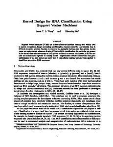
The input video in our system is in YCbCr colour space. Y is the luminance component and Cb and Cr are the bluedifference and red-difference chroma components. The YCbCr colour space was developed as part of ITU-R BT.601 during the development of a word-wide digital component video standard. If all possible colours in YCbCr space in a 24-bit image are quantised, there are 2563 bins. Such a histogram would be sparsely populated. Very fine quantization of the colour space is probably unjustified for images in which the illumination may be variable, and there is additional noise on the colour video. 16 bins histogram for each colour of YCbCr is reasonable, but it still needs huge memory for hardware implementation. Therefore, we use a much coarser quantization of the colour space, 8-bin colour histogram. Each COIL image is transformed into YCbCr space and a normalized vector (the sum of the vector =1) of 83=512 components is obtained. Figure 2 shows an example of
normalized 8-bin colour histogram SVM vector of the red object. If we increase the number of bins, the computation time will dramatically increase.
Figure 2. The 8-bin 3D colour histogram SVM vector of the red object.
We choose γ =1, there are only parameter C need to be determined while use the radial basis function (RBF) kernel, and two parameters C and d for polynomial kernel. It is not know beforehand which C is the best for our problem. In order to obtain a good C so that the classifier can accurately predict unknown data, a “grid-search” on C and d (for example C = 2−5 ,2−3 ,L,215 , d=1,2,3) on a half-training/halftesting methodology was used. The way is to separate training data into two parts, one is considered unknown in training the classifier, the other was used to predict accuracy that reflect the performance on classifying unknown data. The reason why we prefer the grid-search is that the method can avoid doing an exhaustive parameters search by approximations or heuristics, and it can be easily parallelized because each parameter is independent.
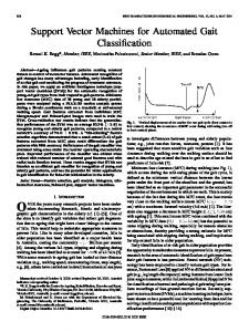
Figure 4 shows our own real data, where three different vehicle types and colors are illustrated (black car, white HGV and red van). The data was collected from real time video. The colour is not as good as in the COIL database, because they are from an outside scene. Some parts of the vehicle which specularly reflect the ambient light appear changed in color. Table 1 gives experiment results with the associated confusion matrix given in Table 2. The results were obtained using OVA with a polynomial kernel, and parameter settings C=1000 and d=2. From the confusion matrix, we know that, from 51 black vehicles, the system predicts 50 as black and only 1 as white. For 110 white vehicle, the system predict 103 as white and 7 as black. The classifier has 100% recognition rate for the red vehicle.
Figure 4. Three different vehicle types and colors (black car, white HGV and red van) TABLE I. Colour Black White Red
COLOUR CLASSIFICATION RESULTS USING REAL DATA Number of vehicle 101 220 64
TABLE II. Black White Red
V.
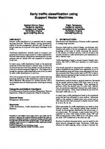
Figure 3. Images with Gaussian white noises mean 0 and variances are 0.05, 0.1, 0.2, 0.5, respectively (order from left to right).
For colour classification experiments, there are 216 blue object images, 288 red, green and yellow object images. Each of them randomly segregated into two sets. Each set include half samples was used separately as a training set and testing set. In order to test the robustness of the algorithm, we add Gaussian white noises with mean 0 and variances are 0.05, 0.1, 0.2, 0.5, respectively. The intensity of the image is normalized ranging from 0 to 1. Figure 3 shows some samples of noised image. Even images with noises variance=0.2, sensitivity and specificity of each colour are still 1.0. That means the method can get 100% correct results. For the image with variance=0.5, the mean of sensitivity=0.999, the mean of specificity=0.998.
Sensitivity
Specificity
0.882 0.916 0.987
0.891 0.832 0.987
CONFUSION MATRIX Black 50 7 0
White 1 103 0
Red 0 0 32
SHAPE CLASSIFICATION
Our system not only classifies different vehicle colors, but also different vehicle types, such as car, van and HGV. The foreground blob containing the vehicle is obtained using a background subtraction method based on a Gaussian mixture model [28]. We extract a simple silhouette shape vector, so that we can implement our system easily on embedded hardware. The feature vector components include size, aspect ratio, width and solidity of the vehicle foreground blob. The size and width is the value after normalization using the size of the license plate. We assume that the size of the license plate is 1 unit. The accuracy of both OVA and OVO is given in Table 3 and associated confusion matrices are given Table 4. From these tables, we know that OVO and OVA do not have significant differences in performance, but OVO performance is slight better than that of OVA on our data, especially for van classification. For our real time hardware system implementation, we chose OVA, to save computation complexity and running time.
TABLE III.
THE ACCURACY OF OVA AND OVO
[7]
Method
OVO Sensitivity Specificity
OVA Sensitivity Specificity
[8]
Car Van HGV
0.852 0.655 0.735
0.938 0.841 0.882
[9] [10]
TABLE IV.
Car Van HGV
Car OVA
91 9 3
THE CONFUSION MATRICES OF OVA AND OVO OVO
Van OVA
92 12 4
10 56 24
[11]
OVO
HGV OVA
OVO
9 67 21
0 27 34
0 13 36
[12]
[13]
VI.
CONCLUSIONS AND DISCUSSION
We have presented a method to perform automatic vehicle recognition and classification. The moving vehicle blob was segmented from static background using a Gaussian mixture model background subtraction algorithm. It is a two-step algorithm. The first step is colour recognition. In order to save memory space and computation complexity for real time hardware system implementation, the system uses a 8-bin colour (YCbCr space) histogram as SVM vector. The system obtained 100% correct recognition for common colors (green, red, blue, yellow) in the COIL database. The second step is type recognition. The type vector components are size, aspect ratio and solidity of the foreground (vehicle) blob. The data are from real road-side cameras, but the image quality is not as good as COIL’s, as they are all outside scenes. Some images are blurred, because of the camera vibration (strong wind). Moreover, the color of some vehicles appears to be changed due to very strong sunlight and specular surface reflection. Despite these challenging conditions, the average type sensitivity of OVO and OVA are 0.759, 0.687, respectively. The average type specificity of OVO and OVA are 0.887, 0.858, respectively. The average colour sensitivity and specificity of OVA are 0.956 and 0.971, respectively.
[14]
[15]
[16]
[17]
[18]
[19]
[20]
[21]
ACKNOWLEDGMENT This paper was supported by the UK Technology Strategy Board project, CLASSAC, and Cybula Ltd. The authors also thank Columbia Object Image Library for their COIL data. REFERENCES [1] [2] [3] [4] [5] [6]
V. Vapnik and A. Lerner, “Pattern recognition using generalized portrait method,” Automation and Remote Control, 24, pp. 774-780, 1963. V. Vapnik and A. Chervonenkis, “A note on one class of perceptrons,” Automation and Remote Control, 25, 1964. O.L. Mangasarian, “Linear and nonlinear separation of patterns by linear programming,” Operations Research, 13:pp. 444-452, 1965. O.L. Mangasarian, “Muti-surface method of pattern separation,” IEEE Transactions on Information Theory IT-14, pp. 801-807, 1968. O.L. Mangasarian, “Nonlinear Programming,” McGraw-Hill, New York, 1969. V.Vapnik, “Estimation of Dependences Based on Empirical Data,” Springer, Berlin. 1982.
[22] [23]
[24]
[25] [26]
[27]
[28]
V. Vapnik, “The Nature of Statistical Learning Theory,” Springer, New York. 1995. C. Cortes and V. Vapnik, “Support vector network,” Machine Learning, vol. 20, pp. 1-25, 1995. V. Vapnik, “An overview of statistical learning theory,” IEEE Transaction on neural networks, vol. 10, No. 5, pp. 988-999, 1999. N. Baek, S.-M. Park, K.-J. Kim, S.-B. Park, “Vehicle Color Classification Based on the Support Vector Machine Method”, ICIC 2007, CCIS 2, pp. 1133–1139, 2007. A. Ambardekar, M. Nicolescu, G. Bebis, “Efficient Vehicle Tracking and Classification for an Automated Traffic Surveillance System,” Signal and Image Processing, August 2008. Ma, W. E. L. Grimson, “Edge-based rich representation for vehicle classification”, International Conference on Computer Vision, 2006, pp. 1185-1192. C. Zhang, X. Chen, W.-B. Chen, “A PCA-based Vehicle Classification Framework”, International Conference on Data Engineering Workshops (ICDEW'06), 2006. M. Pontil and A. Verri, “Support vector machines for 3D object recognition,” IEEE Transaction on Pattern Analysis and Machine Intelligence, Vol. 20, No. 6, pp. 637-646, 1998. R.J. Vanderbei, “LOQO: An interior point code for quadratic programming,” Optimization Method and Software, vol.12, pp. 451-484, 1999. E. Osuna, R. Freund and F. Girosi, “Support Vector Machine: Training and Applications. Technical Report: AIM-1602, Massachusetts Institute of Technology, Cambridge, USA, 1997. F. Girosi, “An equivalence between sparse approximation and support vector machines,” Technical Report: AIM-1606. Massachusetts Institute of Technology, Cambridge, USA, 1997. O. Chapelle P. Haffner and V. Vapnik, “Support vector machines for histogram-based image classification,” IEEE Transaction on Neural newworks, Vol. 10, No. 5, pp. 1055-1064, 1999. V. Blanz, B. Scholkopf, H. Bulthoff, C. Burges, V. Vapnik and T. Vetter, “Comparison of view-based object recognition algorithms using realistic 3D models,” In Artificial Neural Networks – ICANN’96, pp. 251-256, Berlin, Springer Lecture notes in Computer Science, Vol. 1112, 1996. B. Scholkopf, C. Burges and V. Vapnik, “Extracting support data for a given task,” In U. M. Fayyad and R. Uthurusamy, editors, In the Proceedings of the First International Conference on Knowledge Discovering & data Mining, AAAI Press, Menlo Park, CA, pp. 252-257, 1995. F. Melgani, L. Bruzzone, “Classification of hyperspectral remote sensing images with support vector machines,” IEEE Transaction on Geoscience and Remote Sensing, 42, pp. 1778-1790, 2004. R. Rifkin and A. Klautau, “In defense of one-vs-all classification,” Journal of Machine Learning Research, 5, pp. 101-141, 2004. G. Anthony, H. Gregg and M. Tshilidzi, “Image classification using SVMs: one-against-one vs one-against-all,” In Proceedings of the 28th Asian Conference on Remote Sensing. 2007. Allwein E.L., Schapire R.E. and Singer Y. Reducing multiclass to binary: A unifying approach for margin classifiers. Journal of Machine Learning Research, vol.1, pp. 113-141, 2000. J. Furnkranz, “Round robin classification,” Journal of Machine Learning Research, vol. 2 pp. 721-747, 2002. C. Hsu and C. Lin, “A comparison of methods for multi-class support vector machines,” IEEE Transaction on Neural Networks, 13: 415-425, 2002. H. Murase and S.K. Nayar, “Visual learning and recognition of 3-D object from appearance,” International Jornal of Computer Vision, Vol. 14, pp. 5-24, 1995. Z. Zivkovic, F. Heijden, “Efficient adaptive density estimation per image pixel for the task of background subtraction,” Pattern Recognition Letters. 27(7), pp. 773-780, 2006.