Mar 3, 2016 - In the case of an electric/magnetic field or a perfect fluid, the source ...... Principles of Mechanics 4th edn (Toronto: University of Toronto Press).
Home
Search
Collections
Journals
About
Contact us
My IOPscience
Classifying Einstein's field equations with applications to cosmology and astrophysics
This content has been downloaded from IOPscience. Please scroll down to see the full text. 1995 Class. Quantum Grav. 12 2525 (http://iopscience.iop.org/0264-9381/12/10/012) View the table of contents for this issue, or go to the journal homepage for more
Download details: IP Address: 129.16.201.217 This content was downloaded on 03/03/2016 at 14:20
Please note that terms and conditions apply.
Class. Quantum Grav. 12 (1995) 2525–2548. Printed in the UK
Classifying Einstein’s field equations with applications to cosmology and astrophysics Claes Uggla†k, Michael Bradley‡ and Mattias Marklund§ † Department of Physics, Stockholm University, Box 6730, S-11385 Stockholm, Sweden and Department of Physics, Lule˚a University of Technology S-95187 Lule˚a, Sweden ‡ Department of Physics, Ume˚a University, S-90187 Ume˚a, Sweden § Department of Plasma Physics, Ume˚a University, S-90187 Ume˚a, Sweden Received 19 January 1995, in final form 24 July 1995 Abstract. The field equations for spacetimes with finite-dimensional Hamiltonian dynamics are discussed. Examples of models belonging to this class are the cosmological spatially homogeneous models, the astrophysically interesting static spherically symmetric models, static cylindrically symmetric models, and certain cosmological self-similar models. A number of different sources are considered. Although these models arise from quite different physical contexts, their field equations all share a common mathematical structure. This motivates a classification of Einstein’s field equations. Several classification schemes, based on properties under various variable transformations, are presented. It is shown how these schemes can be used to classify dynamical properties of the models and how one can thereby obtain qualitative information. It is also shown how one scheme can be used in order to find symmetries and exact solutions. PACS numbers: 0420, 9530S, 9880H
1. Introduction In this paper the properties of the field equations of two classes of spacetimes will be discussed. These two classes consist of models with homogeneous non-null hypersurfaces (hypersurface-homogeneous (HH) models) and models with timelike surfaces admitting a transitive self-similar group which have two commuting spacelike Killing vectors (timelikeself-similar models (TSS)). The sources considered here are perfect fluids, electric or magnetic fields, scalar fields or a combination of these. A cosmological constant can also be included. For all these models the Einstein field equations reduce to ordinary differential equations. Only models with a Hamiltonian formulation for the field equations will be considered. The purpose of this paper is to discuss and classify the different types of Hamiltonian problems which arise in HH and TSS dynamics, i.e. we are going to classify Einstein’s field equations for these models. Note that this classification has nothing (or at least very little) to do with a classification of the underlying spacetimes which give rise to the Hamiltonians. We are also going to show that this is a useful thing to do, by giving explicit applications. The outline of the paper is the following. In section 2 we present a number of Hamiltonians, written in a certain ‘standard form’. The Hamiltonians arising in HH and k Supported by the Swedish Natural Science Research Council. c 1995 IOP Publishing Ltd 0264-9381/95/102525+24$19.50
2525
2526
C Uggla et al
dynamics can be divided into two classes: SE Hamiltonians and non-SE Hamiltonians. are Hamiltonians that can be written in a form where the kinetic part is Lorentzian and the potential is a sum of exponentials (motivating the notation ‘SE’). The highly particular structure of SE-Hamiltonians motivates various classification schemes of the Hamiltonian which exploits this structure. Such classification schemes are discussed in section 3. In section 4 we discuss, in detail, the example of two-dimensional SE-Hamiltonians with a potential consisting of two positive exponential terms. As an application, we reformulate the field equations to a regularized dynamical system of differential equations and show that there is a close connection between the classification schemes and various qualitative properties of the dynamical system, e.g. the number of equilibrium points. The classification schemes presented in section 3 are not particularly useful for nonSE-Hamiltonians. To deal with problems which include non-SE-Hamiltonian cases, we introduce yet another classification scheme in section 5. This classification scheme is based on equivalence under general point transformations of the dependent variables of the Hamiltonian, in contrast to the ones introduced in section 3 which exploit the Poincar´e group associated with the Lorentzian kinetic part of the SE-Hamiltonians. To implement this scheme we first reformulate the field equations to a set of geodesic equations of the so-called Jacobi geometry which encodes the entire dynamical content of the Hamiltonian and thus also of the field equations. Note that the Jacobi geometry has nothing to do with the original spacetime geometry. We then classify the Jacobi geometry by applying a procedure developed by Cartan [1] and others [2–4] for classifying geometries. Many interesting Jacobi geometries are two-dimensional. This motivates a complete classification of two-dimensional geometries. This classification is given in the appendix. The present classification scheme can be used to find symmetries of the Hamiltonian. In particular, we give criteria for such symmetries in the two-dimensional case. In section 6 we apply the results from section 5 and the appendix in order to show, as an application, how one can find Hamiltonian symmetries for problems describing flat isotropic scalar field models, and how these symmetries give rise to exact solutions. TSS
SE-Hamiltonians
2. Line elements and Hamiltonians The models which we will consider have line elements which can be written as [5, 6] ( �N (λ)2 dλ2 + gab (λ)ωa ωb HH models 2 (2.1) ds = 2 2 2 2 2 2p1 2 2 2p2 2 2 TSS models, t N (λ) dλ − R3 (λ) dt + t R1 (λ) dx + t R2 (λ) dy where p1 and p2 are constants that satisfy certain conditions (these are given below for the perfect fluid case). The constant � takes the values −1 and 1 for the spatially homogeneous (SH) models and the static HH models, respectively. A particular choice of N corresponds to a choice of independent variable. The 1-forms ωa (a = 1, 2, 3) describe the different symmetry groups which act transitively on three-dimensional hypersurfaces. The HH models admit simply transitive or multiply transitive (MT) homogeneity groups. The models which admit a simply transitive three-dimensional homogeneity group are called Bianchi models, for which the 1-forms may be chosen to satisfy, dωa = − 12 C a bc ωb ∧ ωc , where C a bc are the components of the structure constant tensor of the Lie algebra of the homogeneity group. The Bianchi models are divided into two classes, class A and class B, according to the vanishing or non-vanishing of the trace C b ab . For the class A models one can choose C a bc = n(a) �abc , where the parameters n(a) characterizing the various symmetry types can be chosen to have the following values: Bianchi type I, n = (0, 0, 0); type II,
Classifying Einstein’s field equations
2527
n = (0, 0, 1); type VI0 , n = (1, −1, 0); type VII0 , n = (1, 1, 0); type VIII, n = (1, 1, −1); type IX, n = (1, 1, 1). Explicit coordinate representations of the 1-forms can be found in [7]. Class B models which admit a Hamiltonian formulation will be discussed below. Among the Bianchi models there is a special family which admits MT symmetry groups. There are also MT models which do not admit a simply transitive subgroup (i.e. they are not Bianchi models); the most prominent ones are the SH Kantowski–Sachs models and the static spherically symmetric models. The MT models will be discussed below. When it comes to giving explicit expressions for the line elements and deriving the Hamiltonians, it is convenient to divide the models into diagonal HH models, diagonal TSS models, and non-diagonal HH models. The non-diagonal models are, in general, quite complicated. For simplicity we will only consider the stationary cylindrically symmetric case. Below we collect a number of Hamiltonians which have been derived previously in [5, 6]. We refer to [5] for a detailed discussion of how to obtain the Hamiltonians. The Hamiltonians which we consider have the usual form L = T − U, H = T + U . However, the Hamiltonian must vanish as a consequence of one of the field equations. This leads to the Hamiltonian constraint H = 0. From the expression for H in terms of the velocities, one can read off the Lagrangian as well by a simple change of sign. When deriving the Hamiltonians one wants to express them as simply as possible. To achieve this goal, one chooses new variables which respects the symmetries of the kinetic part of the Hamiltonian (see [5]).
2.1. Diagonal hypersurface homogeneous models The possibility of choosing the timelike direction along different axes in the static case yields an abundance of models. To avoid being lost in details, the signature freedom will be restricted by requiring ω1 and ω2 to be spacelike. This leads to the line element � � ds 2 = � N (λ)2 dλ2 − R3 (λ)2 (ω3 )2 + R1 (λ)2 (ω1 )2 + R2 (λ)2 (ω2 )2 .
(2.2)
The most notable simply transitive models belonging to this class are the SH models and the static Bianchi type I cylindrically symmetric models. The diagonal class A models contain as a special case the diagonal locally rotationally symmetric (LRS) models, characterized by n(1) = n(2) and R1 = R2 . Another overlapping class of models is the diagonal MT models which are characterized by ω3 = dx 3 , R1 = R2 , and where ω1 ⊗ ω1 + ω2 ⊗ ω2 is a Riemannian 2-metric of constant curvature σ ∈ {1, 0, −1}. (These by themselves will be referred to here as the ‘MT case’.) Among the MT models those with σ = 0 coincide with the LRS Bianchi type I models while the case σ = −1 is an LRS Bianchi type III case contained in the class B models discussed below. The case σ = 1, where no three-dimensional simply transitive subgroup exists, corresponds to the SH Kantowski–Sachs (KS) case and the static spherically symmetric models. For simplicity we will only consider SH class B models. The SH diagonal class B models are characterized by structure constants of the form C 1 31 = a +q, C 2 32 = a −q, a 2 = −hq 2 , and an algebraic constraint among the three scale factors Ra [7, 10, 11]. The variables a Ra = eβ may be parametrized in a way which reflects the algebraic structure of possible constraints and which in addition makes the kinetic energy in the Hamiltonian ‘conformally
2528
C Uggla et al
flat’. The parametrizations are the following [12, 13]: √ 0 1 1√ 3 β + β 1 1 − 3 1 β− 0 β 1−2 β2 = β3 � 0 � 1 − c(q − 3a) β 1 − c(q + 3a) β× 1 2cq
class A,
MT
cases, (2.3)
type V and VIh ,
where c = (q 2 + 3a 2 )−1/2 . One can choose q = 0, a = 1 for type V and q = 1 for type VIh as canonical structure constant values. The class A limit of type VI0 arises when a → 0. The above representation is adapted to the LRS models for which β − = 0. The kinetic part of the gravitational Hamiltonian takes the form (2.4) T(G) = 1 xηAB β˙ A β˙ B = 1 x −1 ηAB pA pB , 2
2
where ηAB = ηAB in each case are the orthonormal components of the Minkowski metric, −η00 = η++ = η−−− = η×× = 1, and the indices A, B, . . . take values from the sets {0, +, −} and {0, ×} depending on the context. In the above expression we have introduced the function x [14] which is related to N by the relation 0
x = 12e3β /N .
(2.5)
A choice of x thus represents a choice of independent variable. The choice x = 1, which simplifies the kinetic part as far as possible, is denoted as the ‘Taub slicing gauge choice’ since Taub introduced this gauge choice in the SH context [15]. The potential energy has a contribution U(G) from the gravitational field and contributions from the various sources. We will consider some typical sources: a cosmological constant, an electric or magnetic field along the distinguished (third) spatial direction in the SH case and along the λ-direction in the static case [5], single or multiple non-interacting perfect fluids, and scalar fields. A scalar field φ contributes an additional term to the kinetic energy (2.6) T(S) = 12 x β˙† 2 = 12 x −1 p†2 , √ † where β = (1/ 12)φ. In the case of an electric/magnetic field or a perfect fluid, the source equations can be solved and used to express the potential in terms of metric variables as discussed elsewhere [5]. The 4-velocity uα of the perfect fluid source is orthogonal to the SH hypersurfaces in the SH case and aligned with the third (timelike) direction in the static case. For simplicity we will only consider the equation of state p = (γ − 1)ρ where p is the pressure, ρ the energy density, and γ a constant. The gravitational and source potentials for the various models are 0 12x −1 e4β V ∗ class A 0 + U(G) = 24�σ x −1 e4β −2β MT −1 −2 4(β 0 −cqβ × ) 24x c e SH class B, +
+
+
V ∗ := 12 e4β h− 2 + �n(3) e−2β h+ + 12 (n(3) )2 e−8β , √
√
−
U(3) = −24�x
−1 6β 0
e
3,
(2.7)
−
h± := n(1) e2 3β ± n(2) e−2 3β , ( 0 24κx −1 ρ(0) e3(2−γ )β U(fluid) = 0 + 24x −1 κp(0) e[−(6−5γ )β +2γβ ]/(γ −1) U = −24�x
� = −1, p = (γ − 1)ρ � = 1, p = (γ − 1)ρ , 1 < γ ,
−1 2 2(β 0 −2β + )
ee
,
U(S) = −24�x −1 e6β V(S) (β † ) , 0
Classifying Einstein’s field equations
2529
where U(3) is the potential arising from a cosmological constant 3; U(em) is the potential corresponding to an electric or magnetic field; U(S) is the potential arising from a scalar field potential V(S) ; and where ρ(0) , p(0) and e2 are integration constants of the source equations. 2.2. Timelike-self-similar models The only source to be considered in the context of diagonal TSS models is a perfect fluid with p = (γ − 1)ρ as equation of state with the constant parameter γ taking values in the interval 1 < γ < 2. The fluid velocity is assumed to be tangential to the self-similar group orbits. The constants p1 and p2 , appearing in the line element (2.1), are given by p1 + p2 = (2 − γ )/γ ,
p2 − p1 = m/γ ,
(2.8)
where m is an arbitrary non-negative parameter. It is useful to define a constant k by k = −m2 + (2 − γ )(7γ − 6). This constant can be positive or negative depending on the values of m and γ . The case k = 0 is forbidden by the Hamiltonian constraint H = 0 so only two cases arise, k > 0 or k < 0. In the case k > 0 the kinetic part of the Hamiltonian is positive-definite [6]. Here only the Lorentzian k < 0 case will be considered. For this case it is convenient to define the quantity q by k = −q 2 . The single constraint yields β 3 = [(p1 − 1)β 1 + (p2 − 1)β 2 ]/(p1 + p2 ). Introducing the variables β˜ 0 = q[β 1 + β 2 ]/[γ (p1 + p2 )] , β˜ + = [−2γp2 β 1 + 2γp1 β 2 ]/[γ (p1 + p2 )] , (2.9) leads to a Hamiltonian [6] � � ˜0 H = 12 x −(β˙˜ 0 )2 + (β˙˜ + )2 + 12 x −1 q 2 γ −2 e2(2−γ )β /q + U(source) = 0 ,
(2.10)
where N, occurring in (2.1), is given by N = x −1 eβ +β +β [6]. (Here it is convenient to use a new definition for x, differing by a factor of 12 from the HH case.) The fluid potential is given by [6] 1
2
3
˜ ˜ 0 +b˜+ β˜ +
U(source) = 2x −1 κp(0) eb0 β
where p(0)
, (2.11) ˜ ˜ is an integration constant and b0 = −q/[2(γ − 1)], b+ = −m/[2(γ − 1)].
2.3. Stationary cylindrically symmetric models As an example of a non-diagonal model we will consider the stationary cylindric vacuum model. Non-diagonal models with one non-diagonal degree of freedom have a constant momentum associated with an off-diagonal gravitational cyclic variable. This naturally leads to a reduced Hamiltonian for the diagonal degrees of freedom with an effective potential left behind in the kinetic part of the Hamiltonian. This is analogous to the centrifugal potential which appears in the central force problem. The stationary cylindrically symmetric models have a line element which can be written as [16] 1
2
3
ds 2 = N 2 dλ2 − e2β ( dt + C dφ)2 + e2β dφ 2 + e2β dz 2 ,
(2.12)
a
where β , N and C are functions of the independent variable λ which is interpreted here as a radial coordinate ordinarily denoted by the symbol ρ. Expressing the variables β a in terms of the β 0,± parametrization, the vacuum Hamiltonian assumes the explicit form √ − � H = 1 x ηAB β˙ A β˙ B + 1 e4 3β C˙ 2 = 0 . (2.13) 2
12
The momentum pC associated with the cyclic variable C is constant, leading to, C˙ = √ −1 −4 3β − pC , and the reduced Hamiltonian 12x e √ − (2.14) H = 12 xηAB β˙ A β˙ B + 6x −1 e−4 3β pC2 = 0 .
2530
C Uggla et al
2.4. The mathematical structure of finite-dimensional Hamiltonian problems in GR The above examples covers a considerable range of models describing quite different physical situations. For example, in the HH diagonal case one may consider any combination of sources by including the corresponding potential terms in the Hamiltonian, which together with the two possible signs of � leads to numerous spacetime models. For all cases one can reduce the Hamiltonian to one with a ‘conformally flat’ kinetic part: � � H = 12 xηAB β˙ A β˙ B + x −1 UT = x −1 12 ηAB pA pB + UT = 0 . (2.15) The Taub potential, UT , is the value of the total potential in the Taub slicing gauge x = 1. The list of models with a Hamiltonian of this form can be made much longer, for example, tilted perfect fluid models with one off-diagonal degree of freedom also belong to this class (for this, and a number of other examples, see [5]). In all the above cases, except for the models with general scalar field potentials, the Taub potential is a sum of exponentials X i A Ai ea A β . (2.16) UT = i
A Hamiltonian of this type will be referred to as an SE-Hamiltonian (for ‘sum of exponentials’). Problems of this type arise frequently because the gravitational potential and many source potentials are sums of exponentials when expressed in the Taub slicing gauge. Indeed, practically all the literature deals with problems associated with SE-Hamiltonians. However, this is because one chooses to consider only ‘simple’ sources. Generically, sources give rise to non-SE-Hamiltonians. Thus, for example, if one chooses practically any other equation of state than p = (γ − 1)ρ for a perfect fluid, this leads to a non-exponential perfect fluid potential (see [5]). Many have attempted to solve or analyse the field equations of HH and TSS models individually as though they were completely unrelated. However, the Hamiltonian approach reveals the close mathematical relationship which exists between them. Furthermore, the models one usually considers correspond to problems with highly special Hamiltonians. The particular structure exhibited by these models suggest particular classification schemes that show how the various problems are connected. 3. Classification based on Poincar´e and scale transformations The Minkowski metric ηAB , associated with the kinetic part of Hamiltonians of the form H = 12 xηAB α˙ A α˙ B + x −1 UT = 0 ,
(3.1)
plays a key role in determining the dynamical properties of the equations of motion. The variables α are related to the previous β variables by means of transformations leaving the kinetic part invariant while the indices A and B can take any convenient range of values 0, 1, 2, . . . . The invariance of the kinetic part of the Hamiltonian under Poincar´e transformations, also including reflections, and the scale transformation α A → kα A , x → k −2 x, suggests a classification scheme. Problems that can be transformed into each other by means of these transformations are said to be equivalent. Hence, for example, the SH vacuum type II model is equivalent to the static type I perfect fluid models with 1 < γ < 2 under this type of classification.
Classifying Einstein’s field equations
2531
3.1. Classification of SE-Hamiltonians P bi A α A In the SE case, UT = , the system of differential equations is characterized i Bi e i by the constants b A and Bi . Translations in α A result in scalings of the coefficients Bi , thus naturally defining an equivalence class of such coeffients. Lorentz transformations, reflections, and scale transformations yield an equivalence class of bi A coefficients. Thus we have an equivalence class of coefficients Bi , bi A which leads to systems of differential equations with the same mathematical properties. In the SE case it is also useful to consider a less restrictive classification scheme that does not lead to mathematical equivalence but instead leads to classes of problems that share some mathematical properties. An SE-Hamiltonian problem is determined by the coefficients bi A , Bi . Of particular importance is the rank of the matrix b, with coefficients bi A , and the signs of the coefficients Bi . For an n-dimensional problem a rank less than n implies the existence of cyclic coordinates. Of importance is also the causality of the exponents of individual terms, i.e. if ηAB bi A bi B is positive, null or negative. The causality of ‘relative terms’ ηAB (bi A − bj A )(bi B − bj B ) also plays an important dynamical role. Thus one can base a classification scheme on these properties. In the next section such a scheme will be implemented for the case of two positive exponential terms.
4. Application: the case of two positive exponential terms In this section we will deal with the case � � � 1 0 1 1 2 0 2 1� H = 12 x −(α˙ 0 )2 + (α˙ 1 )2 + x −1 D12 eb 0 α +b 1 α + D22 eb 0 α +b 1 α = 0 ,
(4.1)
where ((b1 0 , b1 1 ) 6= (b2 0 , b2 1 )). Note that if the rank of b is 2 one can set the coefficients D1 and D2 to 1 by means of a translation. If the rank is 1, corresponding to the existence of a cyclic coordinate, one can use a translation of the non-cyclic variable to set D1 = D2 . A boost, reflections, and scaling leads to the transformation α¯ 0 = � 0 0s −1 (α 0 − vα 1 ) ,
α¯ 1 = � 1 0s −1 (−vα 0 + α 1 ) ,
α 0 = 0s(� 0 α¯ 0 + v� 1 α¯ 1 ) ,
α 1 = 0s(v� 0 α¯ 0 + � 1 α¯ 1 ) ,
(4.2)
where v < 1 is the boost parameter, s is the scale parameter, � 0,1 = ±1 are the reflection parameters, and 0 = (1 − v 2 )−1/2 . The above transformation together with the definition, x¯ = s 2 x, leads to the Hamiltonian � � � ¯1 0 ¯1 1 ¯2 0 ¯2 1 � H = 12 x¯ −(α˙¯ 0 )2 + (α˙ 1 )2 + x¯ −1 D12 eb 0 α +b 1 α + D22 eb 0 α +b 1 α = 0 , (4.3) where b¯ 1 0 = � 0 s0(b1 0 + vb1 1 ) , b¯ 2 0 = � 0 s0(b2 0 + vb2 1 ) ,
b¯ 1 1 = � 1 s0(vb1 0 + b1 1 ) , b¯ 2 1 = � 1 s0(vb2 0 + b2 1 ) .
(4.4)
Note that it is possible to interchange the potential terms without loss of generality since one can set D1 = D2 by means of a translation. This corresponds to interchanging b1 A and b2 A . Thus we naturally have an equivalence class of problems with identical mathematical properties defined by problems that can be transformed into each other by means of the transformation in (4.2) and by interchanging b1 A and b2 A .
2532
C Uggla et al
4.1. Classification based on properties of the exponential terms A broader classification scheme than the above one can be implemented by using properties of the exponential terms. This type of classification can be introduced in a step by step procedure. The first classification level is based on properties of the individual terms. It turns out to be useful to distinguish if (bi 0 , bi 1 ) = (0, 0), (bi 0 )2 > (bi 1 )2 , or (bi 0 )2 ≤ (bi 1 )2 . We will denote these cases as (0), (T) and (NT), respectively. This then leads to eight classes given in table 1. If a term is of type (T), then one can make a boost with velocity v = −bi 1 /bi 0 ,
(4.5)
so that that exponential term only depends on α¯ 0 . Table 1. Classes based on the properties of individual exponential terms. Term/class
1
2
3
4
5
6
7
8
1 2
0
0
NT
T
NT
NT
T
T
NT
T
0
0
NT
T
NT
T
The next level of classification is based on ‘relative’ properties of both exponential terms. First we make a distinction between the cases determined by the rank of b. In the rank 2 case we divide the models into two categories determined by the causality of ηAB (b1 A − b2 A )(b1 B − b2 B ). If this quantity is timelike (i.e. (b1 0 − b2 0 )2 > (b1 1 − b2 2 )2 ) then one can find a transformation of the type given in (4.2) which leads to a Hamiltonian of the form � � 0� ¯1 1 ¯2 1 � H = 12 x¯ −(α˙¯ 0 )2 + (α˙ 1 )2 + x¯ −1 e2α D12 eb 1 α + D22 eb 1 α = 0 , (4.6) where the boost parameter v is given by v = −(b1 0 − b2 0 )/(b1 1 − b2 1 ) .
(4.7)
For such models there exists a monotonic function that restricts the dynamics considerably and which makes it possible to obtain a qualitative picture of the dynamics [18]. Thus it is natural to make the same classification as in the single-potential discussion in terms of timelike (T) or non-timelike (NT) characteristics. However, it is also useful to make a further distinction within the (T) case. There exists a particular solution if the function ¯1 1 ¯2 1 D12 eb 1 α + D22 eb 1 α , admits a minimum. The condition for this, in the original parameters, is (vb1 0 + b1 1 )(vb2 0 + b2 1 ) < 0 ,
(4.8)
where v is given by (4.7). The existence of a particular solution, corresponding to a minimum, turns out to be important when it comes to dynamical systems analysis. Thus from such a point of view it is natural to distinguish between the (T) case with a minimum (Tm) and the remaining cases ((T) without a minimum, (NT), and (0), corresponding to a matrix, b, with rank 1) denoted by (NTm). These two possibilities taken together with the cases based on individual terms leads to a total of 16 classes. As an application we are now going to recast the Hamiltonian equations into a so-called reduced and regularized form [19, 20] and show how closely connected the equilibrium point (singular point, critical point) analysis is with this type of classification.
Classifying Einstein’s field equations
2533
4.2. Classification and a dynamical systems approach The starting point for the reduction and regularization process will be the Hamiltonian in the Taub slicing gauge (x = 1) � � 1 0 1 1 2 0 2 1 (4.9) HT = 12 −(p0 )2 + (p1 )2 + D12 eb 0 α +b 1 α + D22 eb 0 α +b 1 α = 0 . Solving the Hamiltonian constraint for the second potential term � � 2 0 2 1 1 0 1 1 D22 eb 0 α +b 1 α = 12 (p0 )2 − (p1 )2 − D12 eb 0 α +b 1 α =: F ,
(4.10)
and substituting this expressions into the Hamiltonian equations leads to the unconstrained equations α´ 0 = −p0 , p´ 0 = −b1 0 D12 eb
α´ 1 = p1 , 1
Aα
A
− b2 0 F ,
p´ 1 = −b1 1 D12 eb
1
Aα
A
− b2 1 F ,
(4.11)
where ´ = d/dλT and where λT is the independent variable associated with the Taub gauge x = 1. Note that due to the Hamiltonian constraint the variable p0 cannot vanish and so must have a definite sign. The sign is defined by physics and will thus be determined by the particular situation one is interested in. Introducing the new variables V = p1 /(−p0 ) ,
X = D12 eb
2
0α
0
+b2 1 α 1
/p02 ,
(4.12)
dλT , leads to a two-dimensional and a new independent variable defined by dλ = coupled system of autonomous equations V˙ = (b1 1 + b1 0 )X + (b2 1 + b2 0 V )F¯ , � � X˙ = 2X −(b1 0 + b1 1 V ) + b1 0 X − b2 0 F¯ , (4.13) 1 p 2 0
2 0 2 1 F¯ := 1 − V 2 − X = 2D22 eb 0 α +b 1 α /p02 ,
where ˙ = d/dλ, and a set of decoupled equations α˙ 0 = −2, α˙ 1 = −2V . Note that X and V are bounded and satisfy the inequalities X > 0 and F¯ = 1 − V 2 − X > 0. Even though by definition the variable X and the quantity F¯ are positive, since each is associated with a positive exponential term in the UT potential, it is useful to allow the range of these quantities to be extended to include the value zero. The zero values of these quantities correspond to invariant submanifolds of the above reduced coupled system of differential equations. These submanifolds constitute the boundary of the phase space associated with the system of equations and are of importance in constructing a picture of the general dynamical structure. Therefore the boundaries X = 0, F¯ = 0 which correspond to setting D1 and D2 to 0 in the original Hamiltonian, will be included in order to form a system of differential equations for which the variables take values on a compactified phase space (figure 1). This reduced system of differential equations contains the essential dynamical information of the full problem. Once the solution of this system is known one can obtain α 0 and α 1 by quadratures while p0 and p1 can be obtained from the definitions of the new variables. Note, however, that the integration constants are related by the F¯ -equation in (4.13). Note also that the transformation in (4.2) taken together with an interchange of b1 A and b2 A yields an equivalence class of reduced equation systems, i.e. we can define twodimensional systems to be equivalent if they can be obtained from Hamiltonians with exponential coefficients related by (4.4) and by swapping 1 and 2 in bi A (i = 1, 2). We are now going to show how the classification scheme based on the causality of the exponential coefficients is related to the critical point analysis of the reduced equation system.
2534
C Uggla et al
Figure 1. Reduced phase space diagram.
4.2.1. Qualitative analysis of the reduced system. We are now going to present the equilibrium points, together with the corresponding eigenvalues and eigenvectors, of the two-dimensional reduced equation system: V˙ = (b1 1 + b1 0 )X + (b2 1 + b2 0 V )F¯ , � � X˙ = 2X −(b1 0 + b1 1 V ) + b1 0 X − b2 0 F¯ , F¯ := 1 − V 2 − X ,
(4.14)
where the invariant submanifolds X = 0 and F¯ = 1 − V 2 − X = 0 constitute the boundary of the reduced phase space (figure 1). Equilibrium point C0± : V = ±1 , λ± 1 λ± 2
X=0;
= −2(b
1
= −2(b
2
0
± 1b1 1 ) ,
v1± = (1, ∓1) ,
0
± 1b 1 ) ,
v2±
2
(4.15)
= (∓1, 0) .
These equilibrium points correspond to the invariant submanifolds which correspond to the case with no terms in the potential (D1 = D2 = 0) and they follow directly from the Hamiltonian constraint. X : Equilibrium point C0i
V = −b2 1 /b2 0 , X = 0, b2 0 6= 0 ; � 2 2 � λ1 = (b 0 ) − (b2 1 )2 /b2 0 , v1 = (1, 0) , � 2 2 � 2 2 2 2 λ2 = 2 (b 0 ) − (b 1 ) + b 0 b 1 − b1 0 b1 1 /b2 0 ,
(4.16)
� v2 = b2 0 b1 1 − b1 0 b2 1 , (b2 0 )2 − (b2 1 )2 + 2b2 0 b2 1 − 2b1 0 b1 1 . This equilibrium point is located on the invariant submanifold X = 0. Note that the value of V is equal to the boost parameter value given in (4.5), needed to transform the potential term so that it becomes explicitly timelike. The condition F¯ > 0 yields (b2 1 )2 < (b2 0 )2 while for F¯ = 0 the point coincides with one of the C0± points leading to a bifurcation. Thus we have an equilibrium point iff the D2 term is of type (T).
Classifying Einstein’s field equations
2535
X : Equilibrium point C0ii
V = V0 = constant , λ1 = 0 , λ2 = −2(b
X = 0,
b2 0 = b2 1 = 0 ;
v1 = (1, 0) , 1
0
+ b 1 V0 ) ,
(4.17) v2 = (b
1
1
1
+ b 0 V0 , λ2 ) , 1
where V0 2 < 1 and where we have a bifurcation for V0 2 = 1 since points with V0 = ±1 reduce to the C0± points. This case thus corresponds to the problem where the second potential term is of type (0). The 0 eigenvalue corresponds to the fact that we have a 1-parameter set of equilibrium points. ¯
F : Equilibrium point C0i
V = −b1 1 /b1 0 , X = 1 − (b1 1 /b1 0 )2 , b1 0 6= 0 ; � � λ1 = (b1 0 )2 − (b1 1 )2 /b1 0 , v1 = (b1 0 , 2b1 1 ) , � 1 2 � λ2 = 2 (b 0 ) − (b1 1 )2 + b2 0 b2 1 − b1 0 b1 1 /b1 0 , � � � �� �� v2 = b1 0 b1 1 b2 0 − b1 0 b2 1 , b1 0 − 2b2 0 (b1 0 )2 − (b2 0 )2 .
(4.18)
This equilibrium point is located on the invariant submanifold F¯ = 0. The value of V is equal to the boost parameter value given in (4.5), needed to transform the potential term so that it becomes timelike. The condition X > 0 yields (b1 1 )2 < (b1 0 )2 while for X = 0 the point coincides with one of the C0± points leading to a bifurcation. Thus we have a equilibrium point iff the D1 term is of type (T). X : Equilibrium point C0ii
V = V0 = constant , λ1 = 0 , λ2 = −2(b
X = 1 − V0 2 ,
b1 0 = b1 1 = 0 ;
v1 = (1, −2V0 ) , 2
0
+ b 1 V0 ) ,
(4.19)
v2 = (b
2
2
1
+ b 0 V0 , 2b 0 (1 − V0 )) , 2
2
2
where V0 < 1 and where we have a bifurcation for V0 2 = 1. This case thus corresponds to the problem where the second potential term is of type (0). 2
Equilibrium point Cc : V = −(b1 0 − b2 0 )/(b1 1 − b2 1 ) , X = X0 = [(b2 1 )2 − (b2 0 )2 + b1 0 b2 0 − b1 1 b2 1 ]/(b1 1 − b2 1 )2 , � � √ v± = (v1 , v2± ) , λ± = (c0 ± c1 )/ 2(b1 1 − b2 1 ) ,
b1 1 6= b2 1 ;
c0 := b1 1 b2 0 − b1 0 b2 1 , c1 := c0 2 + 8X0 ((b1 0 )2 − (b1 1 )2 + b2 0 b2 1 − b1 0 b1 1 )(b1 1 − b1 2 )2 , v1 = 2(b v2±
− b 1 )(b √ = c2 ± (b 1 − b 1 ) c1 , 1
0
+b 1
1
1
−b
2
0
2
1
1
−b
1
0
+b
2
0
− b 1 )(b 2
1
1
(4.20)
− b 1) , 2
2
c2 := −(b1 1 )2 b2 0 − 3b1 1 b1 0 b2 1 + 5b1 1 b2 1 b2 0 + 4(b1 0 )2 b2 0 + 3b1 0 (b2 1 )2 � � − 8b1 0 (b2 0 )2 + 4b2 0 (b2 0 )2 − (b2 1 )2 . Note that the value of V is equal to the boost parameter value, given in (4.7), needed to transform the potential to the form of (4.6). Furthermore, the condition that the potential admits a minimum in the α¯ 1 variable taken together with the condition that the boost parameter v satisfies v 2 < 1, i.e. that we have a (Tm) case, are equivalent with the conditions
2536
C Uggla et al
X > 0, F¯ > 0, which corresponds to the existence of an equilibrium point in the interior physical phase space. This equilibrium point thus correponds to the particular solution that is associated with the minimum of the potential. Note also that the above eigenvalues are complex if c1 < 0. From the above discussion we see that the above classification scheme, based on the properties of b, is directly related to the existence of equilibrium points. Moreover, the transition from one class to another corresponds to a bifurcation. Hence a quick glance at the properties of b immediately yields considerable dynamical information. Furthermore, the equilibrium point values of the variable V correspond to the velocities needed to transform the individual potential terms to ‘explicit (T) form’ and the full potential to ‘explicit (Tm)’ form.
4.2.2. Examples of problems with two positive exponential terms. There are a number of problems with two degrees of freedom and two positive exponential terms. However, the class can be enlarged with problems with additional degrees of freedom provided they admit cyclic coordinates which allow them to be reduced to such problems. As an example, consider the static Bianchi type I perfect fluid model. It is described by the Hamiltonian
Table 2. Examples of models with two positive exponential terms. In the table the following abbreviations have been used: I, II, V, VIh , VIII stand for the corresponding Bianchi models; Cyl for cylindrically symmetric; FIso and OIso for the flat and open isotropic models; Sp for the static spherically symmetric model; pf, em, vac, 2pf, stand respectively for perfect † (1) fluid, electric/magnetic field, vacuum, two non-interacting perfect fluids; V(S) = C1 2 eλ1 β , p † † (2) λ β λ β 2 2 2 2 1 2 V(S) = C1 e + C2 e , C3 = 6(4 + κv3 ), q = m − (2 − γ )(7γ − 6) where m is a non-negative parameter that satisfies m2 > (2 − γ )(7γ − 6). Model
�
Source
(α 0 , α 1 ) D12
D22
(b1 0 , b1 1 )
I I I I I I, Cyl I, LRS I, LRS I, LRS I, LRS FIso II II, LRS II, LRS II, LRS V, VIh V, VIh V, VIh OIso Sp Sp VIII, LRS
+1 −1 −1 −1 −1 1 −1 −1 1 −1 −1 −1 −1 −1 −1 −1 −1 −1 −1 1 1 −1 1
pf pf 3>0 em (1) V(S) vac 2pf 3 > 0, pf 3 < 0, pf 3 > 0, em (2) V(S) vac pf 3>0 em pf 3>0 em (1) V(S) pf 3 0 since they are of particular interest when it comes to inflationary models.
Classifying Einstein’s field equations
2543
6.1. Case I The first solution of (6.5) yields the Jacobi metric � � � � z −dt 2 + dz 2 . (6.6) dsJ2 = e2t sinh2k 1+k This metric gives rise to the Ricci scalar, � � z 2k −2t −2(1+k) e sinh . (6.7) R= (1 + k)2 1+k A calculation shows that g µν R,µ R,ν > 0. Thus R is a spacelike coordinate. This implies that it is possible to transform to a basis where R;0 = R;01 = R;10 = 0, which is just the basis used in the above general discussion of the timelike Killing vector case. If we start with the natural frame, ω˜ 0 = et+h(z) dt , ω˜ 1 = et+h(z) dz, and make a general Lorentz boost, one can see that the choice ξ = z/(1 + k) of the boost parameter yields the desired basis. In this frame, we have r 2 3/2 R;00 = (1 + k)R 2 ≡ g(R) . (6.8) R ≡ f (R) , R;1 = −(1 + k) k Inserting these expressions into (5.19) yields a(R) = R k/[2(1+k)] .
(6.9)
Thus it follows from (5.18) that dsJ2 = −R k/(1+k) dS 2 +
k R −3 dR 2 . 2(1 + k)2
A change of coordinates, √ R¯ ≡ 2kR −1/[2(1+k)] ,
(6.10)
(6.11)
transforms the metric to conformally flat form: � ¯ 2 �k � � R −dS 2 + dR¯ 2 . (6.12) dsJ 2 = 2k For all this to be useful, we need a way back to our ‘old’ coordinates t and z. We already ¯ z) (from (6.7) and (6.11)) so we now seek S = S(t, z). This relationship have R¯ = R(t, can be found by noticing that � � ∂S ∂S 0 ¯ ¯ dt + dz ω = a(R) dS = a(R) ∂t ∂z �� � � � � � � z z z t k cosh dt + sinh dz , (6.13) = e sinh 1+k 1+k 1+k from which it follows: � � z 1 t/(1+k) , (6.14) cosh S(t, z) = √ e 1+k d where d ≡ [2k(1 + k)2/k ]−k/(1+k) , and where the gauge feedom has been used to set the integration constant to zero. This leads to ¯ ¯ = 1 (1 + k) ln d(S 2 − R¯ 2 ) , ¯ = 1 (1 + k) ln S + R . t (S, R) z(S, R) (6.15) S − R¯ 2 2 The Killing vector K of the Jacobi metric in (6.6) is given by � � � � � � √ −t/(1+k) ∂ z ∂ z ∂ = (1 + k) de − sinh . cosh K= ∂S 1 + k ∂t 1 + k ∂z
(6.16)
2544
C Uggla et al
6.2. Case II This case is given by the second solution in (6.5), and is completely analogous to case I, apart from the fact that here R is a timelike coordinate, so we just state the results. The metric takes the form � ¯ 2 �k � � R −dR¯ 2 + dS 2 , (6.17) dsJ2 = 2k while the coordinate transformations are given by � � � � z z 1 ¯ z) = √1 et/(1+k) cosh , S(t, z) = √ et/(1+k) sinh , R(t, 1+k 1+k d d
(6.18)
where d and the inverse transformations are the same as in case I. The Killing vector takes the form � � � � � � √ ∂ z ∂ z + cosh . (6.19) K = (1 + k) de−t/(1+k) −sinh 1 + k ∂t 1 + k ∂z 6.3. Hamiltonians and solutions for cases I and II The Hamiltonians of cases I and II look very similar, the only difference being that R is spacelike for I and timelike for II. They can be written as � ¯ 2 �k � � ¯ −S˙2 + R¯˙2 ∓ x −1 p−1 (S, R) ¯ R , H = 12 xp(S, R) 2k
(6.20)
¯ ≡ (1 + k)2 (S 2 − R¯ 2 )−1 (here and below, all upper signs refers to case I and where p(S, R) p the lower to case II). The choice x = p−1 c2 ∓ 2(2k)−k R¯ 2k , where c is a constant of the motion, gives us the solutions explicitly in terms of τ . Solving the equations of motion, we obtain Z dτ ¯ )=τ, R(τ S(τ ) = , (6.21) √ 1 ∓ bτ 2k where b ≡ 2(2k)−k /c2 . These expressions also gives the τ dependenceR for t and z (using (6.15) and (6.18)). To obtain the synchronus time τs we use τs = N dτ , where N = 12x −1 et (see equation (2.11)). This relation gives us Z [±(−τ 2 + S 2 (τ ))](k−1)/2 dτ . (6.22) τs = 12d (1+k)/2 (1 + k)2 c−1 √ 1 ∓ bτ 2k Thus, we can obtain, by some algebra, the full solution to the original problem. Motivated by the inflationary scenario De Ritis et al have studied exact scalar field solutions corresponding to a (slight) generalization of the case k = 2 [25, 26]. Thus there is an overlap between the current models and the ones studied by De Ritis et al. However, all the present models and the models studied by De Ritis et al are special cases of the general Killing tensor cases discussed in [5, 24]. No explicit solution to the full Killing tensor case was given in [5, 24]. The present analysis constitutes the first step towards such a general explicit solution.
Classifying Einstein’s field equations
2545
6.4. Case III This case is the one given in (6.4) that gives a flat metric. The metric can be written as dsJ2 = −dT 2 + dZ 2 if we use one of the transformations � � 1 e(1+C)(z+t) e(−1+C)(z−t) − , (i) C 6= ±1 T (t, z) = 2 1+C −1 + C � � 1 e(1+C)(z+t) e(−1+C)(z−t) + , (6.23) Z(t, z) = 2 1+C −1 + C � � (ii) C = ±1 T (t, z) = 12 ∓z + t + 12 e±2(z±t) , � � Z(t, z) = 12 z ∓ t ± 12 e±2(z±t) . A simple calculation (using the transformations above) gives the Killing vectors ∂T , ∂Z and Z∂T + T ∂Z in the old coordinates. There are other more complicated cases than the present ‘homothetic’ case which can be attacked by the methods developed in section 5 and the appendix. The most prominent example is probably the one describing static spherically symmetric perfect fluid models with an arbitrary equation of state [5]. The conditions yielding Killing vector symmetries (and thus also exact solutions) then translates to conditions on the equation of state. 7. Concluding remarks In this paper we have developed various classification schemes for finite-dimensional problems in general relativity. However, the same schemes can be applied to a whole host of other closely related problems. For example, finite-dimensional problems in higher dimensional theories and non-minimally coupled scalar field theories give rise to Hamiltonians of the same type as discussed here [5]. Can one generalize the present classification schemes to problems with infinite degrees of freedom? Perhaps. The first approaches relies on the conformally Lorentzian structure of the kinetic part. This is a property inherited from the DeWitt metric (or its analogue for timelike slices). In the infinite-dimensional context it is important to note that the DeWitt metric is local. It seems reasonable to assume that it might also play a key role when it comes to determining the dynamical properties of infinite-dimensional problems (there exist several indications that this is the case). Thus classification schemes based on the conformal properties of the DeWitt metric might be useful. Cartan has discussed criteria for the equivalence of a given set of partial differential equations [27, 28]. This discussion is closely related to his approach to the equivalence problem for geometries, used here in the Jacobi context. Thus this seems to be a natural way to proceed when it comes to generalizing the Jacobi classification. Is it useful to attempt to implement classification schemes for infinite-dimensional models? The answer to this question relies on how many physically different models there exists that share a ‘sufficiently’ similar mathematical structure. There are indications that there are a number of models with two commuting Killing vectors that are closely related mathematically, so perhaps such schemes could be useful. We have shown how the equivalence problem approach can be used to find Killing vector symmetries. However, most exact solutions arise from Hamiltonian problems exhibiting the more general Killing tensor symmetries [5]. Unfortunately, there exists no algorithm for finding such symmetries. The Jacobi formulation strengthens the motivation for finding such an algorithm, since it could be applied to Jacobi geometries as well as to spacetime geometries.
2546
C Uggla et al
Appendix We list here the set R p+1 for the different classes of two-dimensional geometries with indefinite signature, (−, +), that exists. Furthermore, the corresponding 1-forms, ω0,1 , in the line element ds 2 = −(ω0 )2 + (ω1 )2 , are given. We use S and R as coordinates. Case I. Constant curvature This is the case where the curvature scalar, R, is a constant. Here no functionally independent quantities are found and hence R completely determines the geometry. No 1-forms are found with the present procedure. However, since the curvature is constant, they are easily found in the literature. Case II. One Killing vector This case has one Killing vector and was treated in detail in a previous section. We list the case when the Killing vector is timelike. Interchange indices, (0 → 1, 1 → 0), to obtain the spacelike case. All components in R p+1 are functions of R and the frame is fixed by requiring R;0 = 0: R = R,
R;0 = 0 ,
R;01 = R;10 = 0 ,
R;1 = f (R) ,
R;00 = g(R) ,
0
R;11 = f (R)f (R) ,
(A.1)
where prime means a derivative with respect to R. In this case one can solve for the following 1-forms: 1 g dR , ω10 = dξ − ω0 . f f The remaining 1-form can be chosen as ω1 =
−
ω0 = e
R
g f2
dR
(A.2)
dS .
(A.3)
The function f (R) may be chosen arbitrary and g(R) is determined by g2 (A.4) = ± 12 Rf , f where the upper (lower) sign in ± refers to the timelike (spacelike) Killing vector case. fg 0 − f 0 g −
Case III. No symmetries, second coordinate in the first derivative This case has no Killing vectors and the second coordinate S (in M) appears already in the first derivative. The case where R is spacelike is listed. The timelike case is obtained as above by interchanging indices. We fix the frame by requiring R;0 = 0. This leads to R = R,
R;0 = 0 ,
R;01 = R;10 = b(R, S) ,
R;1 = S ,
R;00 = a(R, S) ,
R;11 = c(R, S) ,
(A.5)
where a is given by a = c − Sc,S + Scb,S /b + S 2 b,R /b ,
(A.6)
and where a, b and c are related by −
ac 2b2 a2 − + − bb,S + ca,S + sa,R ∓ 12 RS = 0 , S S S
(A.7)
Classifying Einstein’s field equations
2547
where the upper (lower) sign in ∓ refers to R being spacelike (timelike). The 1-forms are given by c 1 1 a b dR , ω1 = dR , ω10 = dξ − ω0 − ω1 . (A.8) ω0 = dS − b bS S S S Case IV. No symmetries, next coordinate in the second derivative This case has no Killing vectors and the second coordinate S appears first in the second derivative. This is possible because the parameter determining the orientation of the frame is found in the first derivative. The frame is fixed as above. This leads to R;1 = f (R) , R;00 = S , R;01 = R;10 = 0 , R = R, R;0 = 0 , R;11 = ff,R ,
R;000 = a(S, R) , 2
S , f where a is given by R;010 = Sf,R +
R001 = ± 12 f R + Sf,R +
R;011 = R;110 = 0 ,
S2 , f
(A.9)
2 R;111 = f 2 f,RR + ff,R ,
a S2 ± 12 Rf a,S + f a,R + Sa,S f,R + a,S = 0 . (A.10) f f (To obtain the case when R is timelike, switch indices and take the lower signs.) The 1-forms are b 1 1 ω0 = dS − dR , ω1 = dR , a af f (A.11) S 0 S2 0 1 b := 2 f R + Sf,R + . ω1 = dξ − ω , f f − af,R − 3S
Case V. R null-like In this case R is null-like. The frame is fixed by requiring R;0 = R;1 = 1. We first show that there are no Killing vectors in this case. If one assumes that R is null-like and that there is one Killing vector, then R p+2 is given by R = R,
R;0 = R;1 = 1 ,
R;00 = R;01 = R;10 = R;11 = f (R) ,
R;000 = R;001 = R;010 = R;011 = R;110 = R;111 = 2f 2 + f,R .
(A.12)
i The Ricci identity R;001 − R;010 = R001 R;i , yields 12 R = 0, i.e. one obtains the flat case and thus a contradiction. Since there are no Killing vectors one can choose coordinates so that
R = R,
R;0 = R;1 = 1 , R;00 = R;01 = R;10 = R;11 = S , 3 S R;000 = R;010 = R;110 = f + S 2 + , (A.13) 2 R 3 S 1 R;001 = R;011 = R;111 = f + S 2 + + R , 2 R 2 where f = f (R) is an arbitrary function of R. The 1-forms are given by � � 2a 2 2 0 ω = 1+ dR − dS , ω1 = (dS − a dR) , ω10 = dξ − S(ω0 + ω1 ) , R R R (A.14) where a = f − 12 S 2 + RS .
2548
C Uggla et al
References [1] [2] [3] [4] [5] [6] [7]
[8] [9] [10] [11] [12] [13] [14] [15] [16] [17] [18] [19] [20] [21] [22] [23] [24] [25] [26] [27] [28]
Cartan E 1946 Lecons sur la Geometrie des Espaces de Riemann 2nd edn (Paris: Gauthier-Villars) Karlhede A 1980 Gen. Rel. Grav. 12 693 Karlhede A and Lindstr¨om U 1983 Gen. Rel. Grav. 15 597 Bradley M and Karlhede A 1990 Class. Quantum Grav. 7 449 Uggla C, Jantzen R T and Rosquist K 1995 Phys. Rev. D 51 5522 Uggla C 1992 Class. Quantum Grav. 9 2287 Jantzen R T 1987 Proc. Int. Sch. Phys. ‘E Fermi’ Course LXXXVI on ‘Gamov Cosmology’ ed R Ruffini and F Melchiorri (Amsterdam: North-Holland) p 61; 1984 Cosmology of the Early Universe ed R Ruffini and L Z Fang (Singapore: World Scientific) p 233 Taub A H and MacCallum M A H 1972 Commun. Math. Phys. 25 173 Misner C W, Thorne K S and Wheeler J A 1973 Gravitation (New York: Freeman) Jantzen R T 1987 Phys. Lett. 186B 290 Rosquist K, Uggla C and Jantzen R T 1990 Class. Quantum Grav. 7 611 Misner C W 1969 Phys. Rev. 186 1319 Uggla C and Rosquist K 1991 Class. Quantum Grav. 7 L279 Jantzen R T 1988 Phys. Rev. 37 3472 Taub A H 1951 Ann. Math. 53 472 Kramer D, Stephani H, MacCallum M and Herlt E 1980 Exact Solutions of Einstein’s Field equations (Cambridge: Cambridge University Press) Jantzen R T 1983 Ann. Phys., NY 145 378 Uggla C, Jantzen R T, Rosquist K and von Zur-M¨uhlen H 1991 Gen. Rel. Grav. 23 947 Rosquist K and Jantzen R 1988 Phys. Rep. 166 89 Uggla C 1989 Analysis of approximate and exact cosmological solutions in general relativity PhD Thesis Stockholm Lanczos C 1970 The Variational Principles of Mechanics 4th edn (Toronto: University of Toronto Press) Abraham R and Marsden J E 1978 Foundations of Mechanics 2nd edn (Reading, MA: Benjamin/Cummings) Uggla C, Rosquist K and Jantzen R T 1990 Phys. Rev. D 42 404 Rosquist K and Uggla C 1991 J. Math. Phys. 32 3412 De Ritis R, Marmo G, Platania G, Rubano C, Scudellaro P and Stornaiolo C 1990 Phys. Rev. D 42 1091 De Ritis R, Marmo G, Platania G, Rubano C, Scudellaro P and Stornaiolo C 1990 Phys. Lett. 149A 79 Cartan E 1945 Les Syst`emes Diff´erentials Ext´eriurs et Leurs Applications G´eom´etriques (Paris: Hermann) Harrison B K and Estabrook F 1971 J. Math. Phys. 12 653