Factorized Solution of Sylvester Equations with Applications in Control∗ Peter Benner†
Abstract Sylvester equations play a central role in many areas of applied mathematics and in particular in systems and control theory. Here we will show how low-rank solutions for stable Sylvester equations can be computed based on the matrix sign function method. We discuss applications in model reduction as well as in observer design. Numerical experiments demonstrate the efficiency of the proposed method.
Keywords. Sylvester equation, matrix sign function, model reduction, observer design.
1
Introduction
Consider the Sylvester equation AX + XB + C = 0,
(1)
where A ∈ Rn×n , B ∈ Rm×m , C ∈ Rn×m , and X ∈ Rn×m is the sought-after solution. Equation (1) has a unique solution if and only if α + β 6= 0 for all α ∈ σ (A) and β ∈ σ (B) [22], where σ (Z) denotes the spectrum of the matrix Z. In particular, this property holds for stable Sylvester equations, where both σ (A) and σ (B) lie in the open left half plane. The anti-stable case, where σ (A) and σ (B) are contained in the open right half plane, is trivially turned into a stable one by multiplying (1) by −1. Sylvester equations have numerous applications in control theory, signal processing, filtering, model reduction, image restoration, decoupling techniques for ordinary and partial differential equations, implementation of implicit numerical methods for ordinary differential equations, and block-diagonalization of matrices, see, e.g., [3, 13, 14, 9, 12, 18, 27] to name only a few references. Many of these applications lead to stable Sylvester equations. Standard solution methods for Sylvester equations of the form (1) are the BartelsStewart method [5] and the Hessenberg-Schur method [13, 17]. The methods are based 1
Supported by the DFG Research Center “Mathematics for key technologies” (FZT 86) in Berlin. Fakult¨at f¨ ur Mathematik, Technische Universit¨at Chemnitz, 09107 Chemnitz, Germany; e-mail:
[email protected]. 2
1
on transforming the coefficient matrices to Schur or Hessenberg form and then solving the corresponding linear system of equations directly by a backsubstitution process. Therefore, these methods are classified as direct methods. Several iterative schemes to solve Sylvester equations have also been proposed; for methods focusing on large sparse systems see, e.g., [9, 20, 28]. The focus in this paper is on a special class of iterative schemes to solve stable Sylvester equations related to computing the matrix sign function. The basic Newton iteration classically used in this context was first proposed for (1) in [25]; see also [6, 19]. It can basically be described by the recursive application of the rational function f (z) = z + z1 to a suitably chosen matrix. Many other polynomial and rational iteration functions can be employed, though. Here, we will focus on a new and special variant of the standard iteration which allows to compute the solution of the Sylvester equation in factorized form directly, given that the constant term C is factored as C = F G, where F ∈ Rn×p , G ∈ Rp×m . Equations of this type arise for instance in model reduction and observer design as discussed in Section 3. The new method is described in Section 2. Numerical experiments reporting the numerical accuracy and performance as compared to standard methods are given in Section 4. Some concluding remarks follow in Section 5.
2
Factorized Solution of Stable Sylvester Equations
The following basic property of the solutions of Sylvester equations is important in many of the above-mentioned applications and also lays the foundations for the numerical algorithms considered here. ¸ Namely, if X is a solution of (1), the similarity transformation · In X , can be used to block-diagonalize the block upper triangular matrix defined by 0 Im ¸ · A C , (2) H = 0 −B as follows:
·
¸ ¸· ¸−1 · In X A C In X = 0 Im 0 −B 0 Im ¸ ¸ · ¸· ¸· · A 0 In X A C In −X . = 0 −B 0 Im 0 −B 0 Im
(3)
Using the matrix sign function of H and the relation given in (3), Roberts derives in [25] the following expression for the solution of the Sylvester equation (1): ¸ · 1 0 X . (4) (sign (H) + In+m ) = 0 I 2 This relation forms the basis of the numerical algorithms considered since it states that we can solve (1) by computing the matrix sign function of H from (2). Therefore, we may apply the iterative schemes proposed for sign function computations in order to solve (1). In this section we review the most frequently used iterative scheme for computing the sign function and adapt this iteration to the solution of the Sylvester equation. 2
2.1
The Newton iteration
The well-known Newton iteration for computing the sign function of a square matrix Z, with no eigenvalues on the imaginary axis, is given by Z0 := Z,
Zk+1 :=
¢ 1¡ Zk + Zk−1 , 2
k = 0, 1, 2, . . . .
(5)
Roberts [25] already observed that this iteration, applied to H from (2), can be written in terms of separate iterations for A, B, and C: ¢ ¡ gA0 := A, Ak+1 := 21 Ak + A−1 , k ¢ ¡ B0 := B, Bk+1 := 12 Bk + Bk−1 , k = 0, 1, 2, . . . , (6) ¢ ¡ −1 , C0 := C, Ck+1 := 21 Ck + A−1 k Ck Bk
thus saving a considerable computational cost and work space. The iterations for A and B compute the matrix sign functions of A and B, respectively. Hence, because of the stability of A and B, A∞ := B∞ :=
lim Ak = sign (A) = −In ,
(7)
lim Bk = sign (B) = −Im ,
(8)
k→∞ k→∞
and if we define C∞ := limk→∞ Ck , then X = C∞ /2 is the solution of the Sylvester equation (1). The iterations for A and B can be implemented in the way suggested by Byers [8], i.e., Zk+1 := Zk −
¢ 1¡ Zk − Zk−1 , 2
with Z ∈ {A, B}. This iteration treats the update of Zk as a “correction” to the approximation Zk . This can sometimes improve the accuracy of the computed iterates in the final stages of the iteration, when the limiting accuracy is almost reached. In some ill-conditioned problems, the usual iteration may stagnate without satisfying the stopping criterion while the “defect correction” iteration will satisfy the criterion. Furthermore, the convergence of both iterations can be improved using an acceleration strategy. Here we use the determinantal scaling suggested in [8] that is given by Zk := ck Zk ,
1
ck = | det (Zk )|− p ,
where p is assumed to be the dimension of the square matrix Z and det (Zk ) denotes the determinant of Zk . Note that the determinant is obtained as a by-product during the inversion of the matrix at no additional cost. The determinantal scaling is easily adapted to be based on the determinants of Ak and Bk for the corresponding iterations. Hence this scaling differs from the one that would be used if the same strategy would be used for the iteration (5) applied to H from (2). 3
A simple stopping criterion for (6) is obtained from (7) and (8). This suggests to stop the iteration if the relative errors for the computed approximations to the sign functions of A and B are both small enough, i.e., if max {kAk + In k, kBk + Im k} ≤ tol,
(9)
where tol is the tolerance threshold. One √ might choose tol = cε for the machine precision ε and, for instance, c = n or c = 10 n. However, as the terminal √ accuracy can not be reached, in order to avoid stagnation it is better to choose tol = ε and to perform 1–2 additional iterations once this criterion is satisfied. Due to the quadratic convergence of the Newton iteration (5), this is usually enough to obtain the attainable accuracy. The computational cost of (6) is dominated by forming the inverses of Ak and Bk , respectively, and the solution of two linear systems for the sequence Ck . If we consider the factorizations of Ak and Bk to be available as a by-product of the inversion, this adds up to 2(n3 + nm(n + m) + m3 ) flops (floating-point arithmetic operations) as compared to 2(n + m)3 flops for a general Newton iteration step for an (n + m) × (n + m) matrix. Thus, e.g., if n = m, iteration (6) requires only half of the computational cost of the general iteration (5). We would obtain the same computational cost had we computed the inverse matrices by means of a Gauss-Jordan elimination procedure and the next matrix in the sequence Ck as two matrix products.
2.2
The factorized iteration
Here we only consider the Ck -iterates for the Sylvester equation (1) with factorized righthand side, i.e., C = F G, where F ∈ Rn×p , G ∈ Rp×m . The Ak - and Bk -iterations remain unaltered. We can re-write th Ck -iteration as follows: £ ¤ F0 := F, Fk+1 = Fk , A−1 F , k k G0 := G,
Gk+1 =
·
Gk Gk Bk−1
¸
.
Even though this iteration is much cheaper during the initial steps if p ≪ n, m, this advantage is lost in later iterations since the number of columns in Fk+1 and the number of rows in Gk+1 is doubled in each iteration step. This can be avoided by applying a similar technique as used in [7] for factorized solution of Lyapunov equations. Let Fk ∈ Rn×pk and Gk ∈ Rpk ×n . We first compute a rank-revealing QR factorization [11] of Gk+1 as defined above, i.e., · ¸ ¸ · Gk R1 , = U RP, R = Gk Bk−1 0 where U is orthogonal, P is a permutation matrix, and R is upper triangular with R1 ∈ Rr×m of full row-rank. Then we compute a rank-revealing QR factorization of Fk+1 U , i.e., ¸ · £ ¤ T1 −1 , Fk , Ak Fk U = V T Q, T = 0 4
where V is orthogonal, Q is a permutation matrix, and T is upper triangular with T1 ∈ Rt×2pj of full row-rank. Partitioning V = [ V1 , V2 ] with V1 ∈ Rn×t , and computing [ T11 , T12 ] := T1 Q,
T11 ∈ Rt×r ,
we then obtain as new iterates Fk+1 := V1 T11 ,
Gk+1 := R1 P.
Then with Ck+1 from (6) we have Ck+1 = Fk+1 Gk+1 . Setting
1 Z := √ lim Gk , 2 k→∞
1 Y := √ lim Fk , 2 k→∞
we get the solution X of (1) in factored from, X = Y Z. If X has low numerical rank, the factors Y and Z will have the corresponding number of columns and rows, respectively, and the storage and computation time needed for the factorized solution will be much lower than for the original iteration (6).
3
Applications
In this section we discuss two applications of the new algorithm to solve Sylvester equations with factorized right-hand side. Both applications considered here trdult from systems and control theory; applications of Sylvester equations with factorized right-hand side in image restoration can be found in [9].
3.1
Observer design
Given the continuous linear time-invariant (LTI) system x(t) ˙ = Ax(t) + Bu(t), y(t) = Cx(t),
t > 0, t ≥ 0,
x(0) = x0 ,
(10)
with A ∈ Rn×n , B ∈ Rn×m , and C ∈ Rp×n , a state observer is a function z : [0, ∞) → Rn such that for some nonsingular matrix Z ∈ Rn×n and e(t) := z(t) − Zx(t), we have lim e(t) = 0.
t→∞
The classical idea of Luenberger [23] to construct a state observer is to find another dynamical system z(t) ˙ = Hz(t) + F y(t) + Gu(t) (11) 5
with solution z(t). If (A, C) is observable and (H, F ) is controllable, then a unique full-rank solution of theSylvester observer equation HX − XA + F C = 0 exists and with G := XB, the solution z(t) of (11) is a state observer for any initial values x0 , z(0), and any input function u(t). If H and F are given, this equation has the discussed structure of low-rank right-hand side as usually, the number p of outputs of the system is much smaller than the dimension n of the state-space.
3.2
Model reduction using the cross-Gramian
If we consider again the LTI system (10), then the task in model reduction is to find another LTI system ˆx(t) + Bu(t), ˆ xˆ˙ (t) = Aˆ t>0 xˆ(0) = xˆ0 , (12) yˆ(t) = Cˆ xˆ(t), t ≥ 0,
ˆ ∈ Rr×m , Cˆ ∈ Rp×r , so that the state-space dimension r of the system with Aˆ ∈ Rr×r , B (12) is much less than n and the output error y(t) − yˆ(t), obtained by applying the same input function u(t) to both systems, is small. One of the classical approaches to model reduction is balanced truncation, see, e.g., [4, 24, 29] and the references therein. This requires the solution of the two Lyapunov equations AWc + Wc AT + BB T = 0,
AT Wo + Wo A + C T C = 0.
(13)
Balanced truncation model reduction methods are then based on invariant or singular subspaces of the matrix product Wc Wo or its square root. In some situations, the product Wc Wo is the square root of the solution of the Sylvester equation AX + XA + BC = 0.
(14)
The solution X of (14) is called the cross-Gramian of the system (10). Of course, for (14) being well-defined, the system must be square, i.e., p = m. Then we have X 2 = Wc Wo if • the system is symmetric, which is trivially the case if A = AT and C = B T (in that case, both equations in (13) equal (14)) [15]; • the system is a single-input/single-output (SISO) system, i.e., p = m = 1 [16]. In both cases, instead of solving (13) it is more efficient to use (14). The new algorithm presented in the previous section is ideally suited for this purpose, particularly in the SISO case, as p = m = 1 is the case yielding the highest efficiency. Moreover, the Bk -iterates in (6) need not be computed as they equal the Ak ’s. This further reduces the computational cost of this approach significantly. Also note that the cross-Gramian carries information of the LTI system and its internally balanced realization if it is not the product of the controllability and observability Gramian and can still be used for model reduction; see [16, 2]. 6
4
Numerical Results
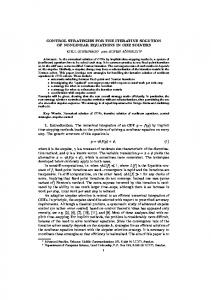
All the experiments presented in this section were performed on an Intel Pentium M processor at 1.4 GHz with 512 MBytes of RAM using Matlab Version 6.5.1 (R13) and the Matlab Control Toolbox Version 5.2.1. Matlab uses ieee double-precision floating-point arithmetic with machine precision (ε ≈ 2.2204 × 10⁻¹⁶ ). Example 4.1 In this example we evaluate the accuracy and computational performance of the factorized Sylvester solver and the Bartels-Stewart method as implemented in the Matlab Control Toolbox function lyap. We construct nonsymmetric stable matrices A, B ∈ Rn×n with eigenvalues λj ∈ R equally distributed between − n1 and −1 as follows: ¡ ¢ ¡ ¢ A = U T diag(λ1 , . . . , λn ) + e1 eTn U, B = V T diag(λ1 , . . . , λn ) + e1 eTn V
where U, V ∈ Rn×n are the orthogonal factors of the QR decomposition of random n × nmatrices. The matrices F ∈ Rn×1 and G ∈ R1×n have normally distributed random entries. Figure 1 shows the residuals and execution times obtained by the two methods. Here, the accuracy is comparable while the execution time of the new method is clearly superior. CPU Times
Residuals
−11
180
10
sign function Bartels−Stewart
sign function Bartels−Stewart
160
120
−12
10
100
sec.
|| A X + X A + BC ||
F
140
80
−13
60
10
40
20
−14
10
0
100
200
300
400
500
600
700
800
900
0
1000
0
100
200
300
400
500
600
700
800
900
1000
n
n
Figure 1: Example 4.1, residuals (left) and performance (measured by CPU time, right) of the factorized Sylvester solver and the Bartels-Stewart method for solving a Sylvester equation with factorized right-hand side.
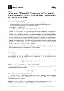
Example 4.2 Here we test the factorized sign function iteration for the cross-Gramian of a SISO system resulting from the semi-discretization of a control problem for a 1D heat equation. This is a test example frequently encountered in the literature [1, 10, 21, 26] and 7
an appropriate test case here The numerical rank of the Gramians of the system is low. Execution times and residuals for the new algorithm are compared to the Matlab solver lyap for several system orders n. Again the obtained results are very promising. CPU Times
Residuals
−10
35
10
sign function Bartels−Stewart
sign function Bartels−Stewart
30
−11
10
|| A X + X A + BC ||
F
25
sec.
20 −12
10
15
10 −13
10
5
−14
10
0
100
200
300
400
500
0
600
0
100
200
300
400
500
600
700
n
n
Figure 2: Example 4.2, residuals (left) and performance (measured by CPU time, right) of the factorized Sylvester solver and the Bartels-Stewart method for computing the crossGramian.
5
Conclusions
We have proposed a new method for solving stable Sylvester equations right-hand side given in factored form as they arise in model reduction problems as well as in observer design. The obtained numerical accuracy as well as the execution time of the new method appear to be favorable when compared to standard solvers. It remains an open problem to give a theoretical foundation to justify the good accuracy, in particular when using the factorized form of the solution.
References [1] J. Abels and P. Benner. CAREX – a collection of benchmark examples for continuous-time algebraic Riccati equations (version 2.0). SLICOT Working Note 1999-14, November 1999. Available from http://www.win.tue.nl/niconet/NIC2/reports.html. [2] R.W. Aldhaheri. Model order reduction via real Schur-form decomposition. Internat. J. Control, 53(3):709–716, 1991. 8
[3] F.A. Aliev and V.B. Larin. Optimization of Linear Control Systems: Analytical Methods and Computational Algorithms, volume 8 of Stability and Control: Theory, Methods and Applications. Gordon and Breach, 1998. [4] A.C. Antoulas. Lectures on the Approximation of Large-Scale Dynamical Systems. SIAM Publications, Philadelphia, PA, to appear. [5] R.H. Bartels and G.W. Stewart. Solution of the matrix equation AX + XB = C: Algorithm 432. Comm. ACM, 15:820–826, 1972. [6] A. N. Beavers and E. D. Denman. A new solution method for the Lyapunov matrix equations. SIAM J. Appl. Math., 29:416–421, 1975. [7] P. Benner and E.S. Quintana-Ort´ı. Solving stable generalized Lyapunov equations with the matrix sign function. Numer. Algorithms, 20(1):75–100, 1999. [8] R. Byers. Solving the algebraic Riccati equation with the matrix sign function. Linear Algebra Appl., 85:267–279, 1987. [9] D. Calvetti and L. Reichel. Application of ADI iterative methods to the restoration of noisy images. SIAM J. Matrix Anal. Appl., 17:165–186, 1996. [10] Y. Chahlaoui and P. Van Dooren. A collection of benchmark examples for model reduction of linear time invariant dynamical systems. SLICOT Working Note 2002–2, February 2002. Available from http://www.win.tue.nl/niconet/NIC2/reports.html. [11] T. Chan. Rank revealing QR factorizations. Linear Algebra Appl., 88/89:67–82, 1987. [12] L. Dieci, M.R. Osborne, and R.D. Russell. A Riccati transformation method for solving linear bvps. I: Theoretical aspects. SIAM J. Numer. Anal., 25(5):1055–1073, 1988. [13] W.H. Enright. Improving the efficiency of matrix operations in the numerical solution of stiff ordinary differential equations. ACM Trans. Math. Softw., 4:127–136, 1978. [14] M.A. Epton. Methods for the solution of AXD − BXC = E and its application in the numerical solution of implicit ordinary differential equations. BIT, 20:341–345, 1980. [15] K.V. Fernando and H. Nicholson. On a fundamental property of the cross-Gramian matrix. IEEE Trans. Circuits Syst., CAS-31(5):504–505, 1984. [16] K.V. Fernando and H. Nicholson. On the structure of balanced and other principal representations of linear systems. IEEE Trans. Automat. Control, AC-28(2):228–231, 1984. [17] G. H. Golub, S. Nash, and C. F. Van Loan. A Hessenberg–Schur method for the problem AX + XB = C. IEEE Trans. Automat. Control, AC-24:909–913, 1979. 9
[18] G.H. Golub and C.F. Van Loan. Matrix Computations. Johns Hopkins University Press, Baltimore, third edition, 1996. [19] W.D. Hoskins, D.S. Meek, and D.J. Walton. The numerical solution of the matrix equation XA + AY = F . BIT, 17:184–190, 1977. [20] D.Y. Hu and L. Reichel. Application of ADI iterative methods to the restoration of noisy images. Linear Algebra Appl., 172:283–313, 1992. [21] D. Kressner, V. Mehrmann, and T. Penzl. CTDSX - a collection of benchmark examples for state-space realizations of time-invariant continuous-time systems. SLICOT Working Note 1998-9, November 1998. Available from http://www.win.tue.nl/niconet/NIC2/reports.html. [22] P. Lancaster and M. Tismenetsky. The Theory of Matrices. Academic Press, Orlando, 2nd edition, 1985. [23] D.G. Luenberger. Observing the state of a linear system. IEEE Trans. Mil. Electron., MIL-8:74–80, 1964. [24] G. Obinata and B.D.O. Anderson. Model Reduction for Control System Design. Communications and Control Engineering Series. Springer-Verlag, London, UK, 2001. [25] J.D. Roberts. Linear model reduction and solution of the algebraic Riccati equation by use of the sign function. Internat. J. Control, 32:677–687, 1980. (Reprint of Technical Report No. TR-13, CUED/B-Control, Cambridge University, Engineering Department, 1971). [26] I.G. Rosen and C. Wang. A multi–level technique for the approximate solution of operator Lyapunov and algebraic Riccati equations. SIAM J. Numer. Anal., 32(2):514–541, 1995. [27] V. Sima. Algorithms for Linear-Quadratic Optimization, volume 200 of Pure and Applied Mathematics. Marcel Dekker, Inc., New York, NY, 1996. [28] E.L. Wachspress. Iterative solution of the Lyapunov matrix equation. Appl. Math. Letters, 107:87–90, 1988. [29] K. Zhou, J.C. Doyle, and K. Glover. Robust and Optimal Control. Prentice-Hall, Upper Saddle River, NJ, 1996.
10