Clearance Based Path Optimization for Motion Planning - CiteSeerX

Clearance Based Path Optimization for Motion Planning Roland Geraerts

Mark H. Overmars

Institute of Information and Computing Sciences Utrecht University, the Netherlands Email: {roland, markov}@cs.uu.nl Abstract— Many motion planning techniques, like the probabilistic roadmap method (PRM), generate low quality paths. In this paper, we will study a number of different quality criteria on paths in particular length and clearance. We will describe a number of techniques to improve the quality of paths. These are based on a new approach to increase the path clearance. Experiments showed that the heuristics were able to generate paths of a much higher quality than previous approaches.

I. I NTRODUCTION Motion planning can be defined as finding a path for an object from a start to a goal configuration without colliding with obstacles in the environment. It has been used in many fields such as mobile robots [1], [2], [3], [4], [5], manipulation planning [6], [7], [8], [9], CAD systems [10], virtual environments [11], protein folding [12] and humanoid robot planning [13]. A commonly used technique for planning paths is the Probabilistic Roadmap Planner (PRM), which was developed at different sites [14], [15], [16]. Due to the probabilistic nature, PRM planners generate low quality paths, i.e. paths that represent many unnecessary motions or do not obey user defined criteria [17], [18]. Also other planning techniques can result in ugly and long paths. In this study, we consider a number of different quality criteria, such as short length and clearance. We investigate how path clearance can be used by heuristics to improve paths such that they meet these criteria. A. Probabilistic Roadmap Method The probabilistic roadmap method consists of two phases: a construction and a query phase. In the construction phase, a roadmap (graph) is built, approximating the motions that can be made in the environment. First, a random configuration is created. Then, it is connected to some useful neighbors. A neighbor is useful if its distance to the new configuration is less than a predetermined constant. Configurations and connections are added to the graph until the roadmap is dense enough. In the query phase, the start and goal configurations are connected to the graph. The path is obtained by a Dijkstra’s shortest path query. See e.g. [19] for a more extensive elaboration of the PRM method. Generally, the paths created with PRM have low quality, which can be explained as follows. First, for efficiency reasons, a roadmap that does not contain cycles (the graph is a tree) can lead to paths containing long detours. Second, the path

consists of straight-line motions between two pairs of nodes of the graph, leading to first order discontinuities at the nodes. Third, because of the random nature of the algorithm, the path contains unnecessary and jerky motions. In this study, we will focus on the optimization of paths which have been generated by a PRM, but the techniques apply to other paths as well. B. Optimization criteria A path should satisfy certain criteria. In general, most applications require a short path, because redundant motions will take longer to execute. For safety reasons, the path should also keep some minimum amount of clearance to obstacles. For example, in a nuclear power plant it is desirable to minimize the risk of heat or radioactive contamination [20]. Notice that these criteria (short path versus clearance) seem to contradict each other: a short path will pull the robot to obstacles while clearance pushes it away. Minimizing the second order gradient of the motions avoids large accelerations and jerky motions such as sharp turns, which increases the controllability. It is also desirable to minimize the number of maneuvers, because this simplifies the action for the driver or controller. Furthermore, it avoids singularities for manipulators [20]. C. Related work Two different kinds of approaches have been proposed to obtain improved paths. First, a path that satisfies some criteria can be chosen from a collection of paths, which we refer to as preprocessing. Second, a path can be optimized in a postprocessing phase. In [21], additional edges are added to the graph in the query phase of the PRM, leading to cycles in the roadmap. In [17], an augmented version of Dijkstra’s shortest path algorithm is used to extract the path (from a graph that contains cycles) satisfying criteria such as length and largest minimum clearance. Unfortunately, there is no guarantee that the extracted path will be optimal after post processing, because the paths are generated randomly. In this paper, we will not consider preprocessing techniques but assume a path in the correct homotopic class has been found. Almost all heuristics that can be found post process the path to reduce its length. The Shortcut heuristic is used most because it seems to work well in practice and is simple to

implement: two configurations c and c0 are chosen on the path. If the straight-line motion between c and c0 is collisionfree, that motion replaces the original part. The configurations can be chosen randomly [22], [10], [23], [24], [25], [26], or deterministically [6], [9], [27]. Also, variants on this heuristic have been proposed [6], [9], [27], [23]. Another class of heuristics creates extra samples around the path [8], [9], [12], [26]. We will show that the Shortcut heuristic can be improved considerably. Also we will show how to (simultaneously) satisfy a clearance criterion.

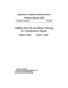
(a) Simple corridor

(b) Corridor

(c) Hole

(d) Wrench

D. Paper outline The paper is organized as follows: in section II, we describe our experimental setup. This includes a description of the paths we will use in our experiments. In section III, we study a simple approach that removes all redundant nodes, resulting in much shorter paths. Clearance is studied in section IV: an algorithm is proposed that increases the clearance of a path. We will show that clearance can be used to decrease the path length for two techniques we propose in section V. In section VI, we combine length and clearance. Finally, we draw some conclusions in section VII. II. E XPERIMENTAL SETUP All techniques that will be described below were integrated in a single motion planning system, called SAMPLE (System for Advanced Motion PLanning Experiments), implemented in Visual C++ under Windows XP. We used the collision detection package Solid [28]. The experiments were run on a 2.66 GHz Pentium 4 processor with 1 GB internal memory. In this study, we restricted ourselves to free-flying objects in a three-dimensional workspace, although we give 2D examples to explain some heuristics. We considered four scenes. In each scene we created a path with the PRM method in such way that an optimization step can not change its homotopic class. In the rest of the paper we show how our different techniques optimize these paths, see Fig. 1. The scenes and their paths have the following properties: Simple corridor This is a simple scene that contains an ugly path traversed by a small cylinder. Many motions are redundant. We expect that they can be removed easily. Corridor This scene forces an elbow shaped object to rotate. The path was created with Gaussian sampling [29], which resulted in little clearance to the corridors. Rotations can only be removed by considering large portions of the path. Hole The moving object consists of four legs and must rotate in a complicated way to get through the hole. Only where the path goes through the hole, the clearance is small. Wrench This environment features a large moving obstacle in a small workspace. The path has some clearance and is relatively short. The moving object is rather constrained at the start and goal. To discuss length and clearance we need a distance measure. We used d = dr + dt where dt denotes the translational distance of the origin of the object and dr denotes the distance traveled by the point of the object furthest from its origin while

Fig. 1.

The four test scenes and corresponding paths

performing the rotation. We calculated dr as follows. Let r1 and r2 be two quaternions and θr = arccos(r1 · r2 ), then dr = radius ∗ min(θr , 2π − θr ). The radii for the Simple corridor, Corridor, Hole and Wrench scene are 1.5, 3.5, 5.5 and 20 respectively. The diagonals of the (bounding boxes of the) scenes are 50, 60, 70, and 275 respectively. In the remainder of the paper, we express path length as a percentage relatively to the ’optimal’ path length because this makes the comparison easier between different optimization techniques. The closer a number approaches zero, the closer to optimal it is. The optimal path lengths were obtained by taking the paths having the minimum length over all experiments conducted and are stated in Table I. Even though we cannot guarantee that these are indeed the optimal paths, we are convinced that they are very close to optimal. (See the full version of this paper for pictures of the optimal paths [30].)

Simple corridor Corridor Hole Wrench

Shortest path length dr dt d 0.3 102.2 102.5 6.2 175.9 182.1 2.2 36.3 38.5 31.9 143.8 175.7

TABLE I T HE SHORTEST LENGTHS OF THE

PATHS

We used Solid for calculating the amount of clearance of the moving object to the obstacles. When we report on clearance, we show the minimum, average and bad clearance. The average clearance gives an indication of the amount of free space in

which the path can be moved without colliding with the obstacles and is calculated as follows. Let π be a path that has been divided to n samples (denoted as πi ) such that the distance between each two sequential samples equals a predetermined constant step size s. (We used the 1/150th fraction of the diagonal size ofP a scene). Then the average clearance equals to n−1 1/Length(π) ∗ i=0 Clearance(πi ). The bad clearance is calculated as follows. Let clmin be the minimum amount of clearance the moving object Pn−1should have to move safely. The bad clearance equals to i=0 clbad (πi ). If Clearance(πi ) < clmin , then clbad (πi ) = clmin −Clearance(πi ), else clbad (πi ) = 0. We set clmin to 0.5. In Table II, we summarize the relative path length (rotational, translational and total) and absolute clearance (minimum, average and bad) of the paths visualized in Fig. 1. As can be seen, the paths are far from being optimal.

Simple corridor Corridor Hole Wrench

Relative path length ∆dr ∆dt ∆d 85500% 151% 400% 4248% 115% 256% 2173% 63% 184% 754% 105% 223%

Path clearance min avg bad 0.16 1.98 3.65 0.00 0.44 269.60 0.36 1.58 0.94 1.23 4.19 0.00

TABLE II T HE RELATIVE LENGTH AND

CLEARANCE STATISTICS OF THE PATHS

III. PATH PRUNING A very simple technique that decreases the path length considerably is to remove all redundant nodes. A node πi of path π is redundant if the straight-line path πi−1 πi+1 is collision-free. See Algorithm III.1 for more details. Algorithm III.1 RemoveRedundantNodes(path π) Require: sequence of n nodes that describe path π 1: for all πi , 0 ≤ i < NumberOfNodes(π)−2 do 2: for all πj , i + 2 ≤ j < NumberOfNodes(π) do 3: if πi πj is collision-free then 4: π ← π\πi+1 5: return π Table III shows the statistics for the paths whose redundant nodes have been removed. The running times of this technique were between 6 and 150 ms. It clearly shows that this simple and fast technique decreases the path length considerably. For example, for the Simple corridor scene, the path is only 27% worse than the optimal path. Note though that, although the translational distance has been improved considerably, the rotational distance is still far from optimal. We will use these paths as input for the heuristics in the rest of this paper. IV. C LEARANCE For many applications, the moving object must maintain a minimum amount of clearance to the obstacles. This criterion

Simple corridor Corridor Hole Wrench

Relative path length ∆dr ∆dt ∆d 6267% 8% 27% 1226% 24% 65% 1655% 19% 112% 570% 65% 157%

TABLE III S TATISTICS FOR ’R EMOVE REDUNDANT NODES ’ HEURISTIC

can be taken into account in each of the two phases of the PRM algorithm. In the construction phase, we could create a roadmap that only contains paths having a minimal amount of clearance clmin . Consider the following approach: one could increase the size of the robot by clmin and use the enlarged robot for collision checking. This has two disadvantages. First, due to the reduction of free space, the narrow passages will be more narrow, making it more difficult or even impossible to find a solution. Second, the roadmap may not be valid for queries that require a clearance larger than clmin . In [31], samples are retracted to the medial axis (MA) of the free (work) space to increase their density in small volume corridors. Such a sample will have 2-equidistant nearest points to the obstacles in the scene, resulting in a locally maximum clearance. We propose a similar approach, but as a post processing step, to retract a complete path to the medial axis. We start with a path whose redundant nodes have been removed. Then, we retract the path to the medial axis. This can yield redundant sub branches, e.g. pieces of the path are traversed twice (see Fig. 2). Those sub branches are removed subsequently. This approach is stated in Algorithm IV.1. Algorithm IV.1 IncreaseClearance(path π) Require: sequence of n nodes that describe path π 1: π 0 ← RetractPath(π) 2: π 00 ← RemoveBranches(π 0) 3: return π 00 In Algorithm IV.2, we retract a free sample to the medial axis of the free space. In line 1, we calculate the closest pair (CPr , CPo ) between the moving object c and the obstacles O. −−−−−→ Then we move in direction CPo CPr until the closest point on the obstacles CPo changes. The step size we use is the distance between the closest pair (CPr , CPo0 ). In lines 7 to 13, we use binary search (with precision δ) to find the sample cmid that has 2-equidistant nearest points to the obstacles. We use Algorithm IV.2 as a step in Algorithm IV.3 to retract a path to the medial axis. In line 1 of Algorithm IV.3, path π is divided to n samples such that the distance between each two sequential samples is at most a predetermined constant step size s. We will retract each sample to the medial axis, except for the start and goal sample. If the distance between two sequential samples of the retracted path π 0 exceeds s, we generate extra samples by applying the algorithm on sub

Algorithm IV.2 RetractEquidistancePoints(sample c) Require: free sample c, obstacles O, precision δ 1: (CPr , CPo ) ← ClosestPair(c, O) 2: CPo0 ← CPo 3: while CPo0 = CPo do 4: c0 ← c 5: c ← c + CPr − CPo0 6: (CPr , CPo0 ) ← ClosestPair(c, O) 7: while Distance(c, c0 ) > δ do 8: cmid ← 21 (c + c0 ) 9: (CPr , CPo ) ← ClosestPair(cmid , O) 10: if CPo0 = CPo then c ← cmid else c0 ← cmid 11: return cmid path {c0i−1 , c0i } until the distance between any two sequential samples is less than s. Algorithm IV.3 RetractPath(path π) Require: sequence of m nodes that describe path π 1: divide π in n samples such that ∀i, d(πi−1 , πi ) ≤ s 2: π 0 ← ∅ 3: for all ci ∈ π, 1 ≤ i < n − 1 do 4: c0j ← RetractEquidistancePoints(ci) 5: if Distance(c0j−1 , c0j ) > s then 6: π 0 ← π 0 ∪ RetractPath(path {c0j−1 , c0j }) 0 7: π ← π 0 ∪ c0i 8: return π 0 The path will now follow the medial axis. As we can see in Fig. 2b, the moving object sometimes traverses the same point twice. This detour is caused by the injective mapping of samples and can be found by looking for reversals in a sub branch of the medial axis. Those redundant motions can be reduced by first removing all redundant nodes, but cannot be avoided completely. Algorithm IV.4 removes those redundant branches in linear time. For each triple {πi−1 , πi , πi+1 }, we remove πi if the distance between πi−1 and πi+1 is less than s. Fig. 2c shows the resulting path which now follows the medial axis without traversing a sub branch twice.

(a) Query path

(b) Retracted path

(c) Removed branches

Fig. 2. The path (a) is retracted to the medial axis and (b) branches are removed (c).

Experiments In the following experiment, we retract the paths of our four example scenes to the medial axis by applying Algorithm IV.1

Algorithm IV.4 RemoveBranches(path π) Require: sequence of n samples along π with step size s 1: i ← 2 2: while i < n do 3: if Distance(πi−1 , πi+1 ) < s then 4: π ← π\πi 5: if i > 1 then i ← i − 1 else i ← i + 1 6: return π on them. The running times for this technique were 0.4, 1.8, 0.6 and 49.4 seconds. The large running time of the Wrench scene can be explained as follows: first, the step size s along the path was small resulting in many calls of Algorithm IV.2. Second, the geometry of this scene and its moving object is more complicated than the other environments. Table IV shows that for all paths the minimum and average clearance was improved (compared to the original paths mentioned in Table II). Furthermore, it shows that nearly all bad clearance was removed, though there is a little amount of bad clearance left in the corridor scene.

Simple corridor Corridor Hole Wrench

Path min 0.66 0.25 0.79 2.11

clearance avg bad 3.32 0.00 1.19 7.86 2.24 0.00 6.96 0.00

TABLE IV S TATISTICS FOR THE M EDIAL A XIS HEURISTIC

We conclude that the technique is successfully able to improve the clearance of a path. In the following section, we show that increasing the amount of clearance can be helpful when optimizing the path length. V. PATH LENGTH We showed in section III that the path lengths were dramatically decreased by pruning the path. They can be decreased further by creating shortcuts. However, redundant motions (like unnecessary rotations) are not removed by those two heuristics. They can only be removed by considering large portions of the path. But if we consider such a large portion, some other degrees of freedom are necessary to navigate around obstacles. Hence, applying the local planner to such a long portion is not going to succeed. The standard optimization technique (Shortcut) replaces pieces of the path by a straight-line segment in the configuration space. In this way, all degrees of freedom (DOFs) are optimized simultaneously. Some of them might be necessary while others are not. The translational DOFs are in particular necessary to guide the object around an obstacle while the rotational DOFs might be less relevant. Consequently, applying the local planner on such part of the path will fail. Calling the local planner to optimize shorter pieces of the path will not remove the rotation either because the two positions on

the path will have rather different orientation. Therefore, the rotation is required, see Fig. 3.

than the length of the Remove redundant nodes heuristic. Note though that there are still many redundant rotational motions.

Simple corridor Corridor Hole Wrench

Relative path length ∆dr ∆dt ∆d 4767% 2% 16% 665% 1% 24% 691% 2% 41% 197% 23% 55% TABLE V

R ELATIVE LENGTHS FOR THE S HORTCUT HEURISTIC (a) Query path

(b) Shortcut

(c) Partial shortcut

Fig. 3. Translation is required to navigate around the obstacle but rotation can only be optimized by considering large portions of the path

We implemented a new technique, called Partial Shortcut, which takes only one degree of freedom (or a group of DOFs) into account in each optimization step, see Algorithm V.1. Let π[0..1] indicate the (continuous) path between c and c0 and let πi [n] denote the value of the ith DOF at position 0 ≤ n ≤ 1. We replace π by a new path π 0 . In this new path all DOFs behave in the same way as in the original path except for f . Algorithm V.1 PartialShortcut(path π) 1: loop 2: c, c0 ← two random configurations on the path 3: π[0..1] → the path between c and c0 4: f ← a random degree of freedom 5: for all n ∈ [0, 1] do 6: for all i 6= f do 7: πi0 [n] ← πi [n] 8: πf0 [n] ← (1 − n)πf [0] + nπf [1] 9: if π 0 is collision free then 10: π ← π0 The disadvantage of the method is that it is relatively slow compared to Shortcut because we often need to check long parts for collision. This can be improved in a number of ways: optimize combinations of DOFs, first check whether a certain replacement improves the path enough before doing the actual tests, and use coherence in the collision checks. We implemented the first improvement and are currently investigating the other two. Experiments We first conducted experiments with the Shortcut heuristic. We must decide how much time this heuristic can spend. The more time it is allowed to run, the shorter the path will be. Because we focus on the maximum quality of the path, we give it more time than is available in real-time applications. Experiments showed that within 5 seconds, the path converged to a (local) optimum. Table V shows that the lengths of the paths decreased dramatically compared to the paths in Table II and III: the path lengths are about two times closer to the optimal length

In the following experiment, we retract the path to the medial axis before we create shortcuts. The rational is that this will give the moving object additional space to move, making it easier to remove redundant motions. Table VI shows the results. Against our expectations, the method did not perform much better. The reason is that situations like in Fig. 3 are not resolved because pushing away does not give enough room.

Simple corridor Corridor Hole Wrench

Relative path length ∆dr ∆dt ∆d 4233% 2% 14% 637% 2% 24% 595% 2% 36% 197% 24% 55%

TABLE VI R ELATIVE LENGTHS FOR THE C LEARANCE +S HORTCUT HEURISTIC

We expect that the Partial shortcut heuristic is able to remove many of those redundant (rotational) motions. Experiments showed that this technique converged within 50 seconds for all scenes. In line 4 of Algorithm V.1, we must choose a particular degree of freedom. For a free-flying robot, there are two kinds of DOFs: translational and rotational ones. We considered rotation as a group, because rotational DOFs are dependent on each other. For translation, one of the three DOFs was chosen randomly. To find out which DOFs we should choose in each iteration step, we split the optimization time in two halves. In each halve, we considered either rotation, translation or a random combination of them. If translation was considered in the first halve of the time, we expected that the robot would ’touch’ the obstacles, which could narrow the range of the rotational freedom. Table VII shows that splitting the optimization time in two halves was worse than choosing them randomly, e.g. the combinations random–random, translation–random and rotation–random performed best. This can be explained by the notion that rotation and translation are dependent on each other. If translation is optimized first, the moving object will ’touch’ the obstacles, e.g. there is no space left for rotation to be optimized. On the other hand, if rotation is optimized first, the resulting translational length after optimizing the path may be longer than the translational part of the optimal path. In the following experiments, we chose the DOFs randomly.

Simple corridor Corridor Hole Wrench

Relative path length – division of optimization time rnd–rnd tra–rot rot–tra tra–rnd rot–rnd 0.5% 2.4% 1.5% 0.8% 0.6% 11.3% 19.3% 20.4% 17.8% 12.2% 22.9% 17.4% 37.9% 15.1% 22.3% 25.9% 30.5% 45.2% 28.6% 28.5%

TABLE VII R ELATIVE LENGTHS FOR THE PARTIAL SHORTCUT HEURISTIC

We applied the Partial shortcut heuristic on the paths. The results are shown in Table VIII. The heuristic was much better able to remove the redundant (rotational) motions than the previous heuristics. Furthermore, the translational lengths of the paths were close to optimal. Notice that the translational path length of the Corridor scene was shorter than the translational path length of the optimal path.

Simple corridor Corridor Hole Wrench

Relative path length ∆dr ∆dt ∆d 200% 0% 1% 392% -2% 11% 377% 1% 23% 142% 0% 26%

Then, we increase the size of the robot by clmin . Finally, we run the Partial shortcut heuristic on the path which only allows changes that are collision-free. Experiments Table X shows the results for the Minimal clearance heuristic. We set clmin to 0.5. We want to remark that we do not know the optimal values for these paths. Compared to the original paths, the lengths are reasonably short and compared to the Clearance+Partial shortcut heuristic, the lengths are (of course) a bit longer. Compared to Table IV, the clearance decreased a little bit.

Simple corridor Corridor Hole Wrench

Relative path length ∆dr ∆dt ∆d 233.3% 3.6% 4.3% 769.4% 9.4% 35.3% 309.1% 5.8% 23.1% 105.3% 0.8% 19.8%

Path min 0.53 0.25 0.60 0.63

clearance avg bad 2.13 0.01 0.84 8.91 1.78 0.00 1.77 0.00

TABLE X S TATISTICS FOR THE M INIMAL C LEARANCE HEURISTIC

TABLE VIII

VII. C ONCLUSION

R ELATIVE LENGTHS FOR THE PARTIAL SHORTCUT HEURISTIC

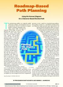
In this paper we investigated techniques to improve path length and clearance. We showed that the path length was decreased considerably if the redundant nodes were removed. The length was further decreased by creating shortcuts. We proposed a new technique (Partial shortcut) that was able to remove considerably more redundant motions. The path length was reduced even further when clearance was added to the path before applying partial shortcuts. We added clearance to a path by retracting it to the medial axis of the work space. This technique was able to optimize paths close to the optimal ones. In Fig. 4, we summarize the results of the experiments we conducted concerning path length. For each path, the absolute values are plotted. We combined the length and clearance criteria and showed that a reasonable short path can be obtained while keeping some minimum amount of clearance. We believe that these new techniques will enhance the quality of motion planners. In future work, we will investigate other robotic systems such as robotic arms. Furthermore, we want to study the trade off between the speed of the techniques and path quality. We will also investigate how additional preprocessing can be used to save time in the post processing phase.

If the path is first retracted to the medial axis, e.g. the path has more clearance, we expect that the technique will produce even shorter paths, because then the moving object will not touch the obstacles which results in more freedom to move. Table IX shows that indeed the total lengths are shorter when the clearance is increased in advance. Only the length of the Simple corridor scene was a little bit deteriorated, which is probably caused by the fact that the path was already close to the optimal path. The table also shows that it is harder to remove rotational motions than translational ones. We will study this further in future work.

Simple corridor Corridor Hole Wrench

Relative path length ∆dr ∆dt ∆d 233% 1% 2% 129% 1% 5% 323% 1% 14% 89% 0% 16%

TABLE IX R ELATIVE LENGTHS FOR THE C LEARANCE +PARTIAL SHORTCUT HEURISTIC

ACKNOWLEDGMENT VI. C LEARANCE

VERSUS SHORT PATHS

In motion planning applications, it is desirable to combine the clearance and short path criteria. While some minimum amount of clearance (clmin ) to obstacles is wanted, the paths should not be too long. We can meet both criteria by finding the shortest path while preserving clmin . First, we retract the path to the medial axis.

The authors would like to thank Dennis Nieuwenhuisen for developing the Callisto collision and visualization toolkit. This research was supported by the Dutch Organization for Scientific Research (N.W.O.). This research was also supported by the IST Programme of the EU as a Shared-cost RTD (FET Open) Project under Contract No IST-2001-39250 (MOVIE - Motion Planning in Virtual Environments).

Path length

600 translation rotation

400 200 0 Initial path Redundant nodes

Shortcut

MA + Shortcut

Partial shortcut

MA+Partial shortcut

Optimal

(a) Simple corridor 750 Path length

translation

500

rotation

250 0 Initial path Redundant nodes

Shortcut

MA + Shortcut

Partial shortcut

MA+Partial shortcut

Optimal

(b) Corridor 120 Path length

translation rotation

80 40 0 Initial path

Redundant nodes

Shortcut

MA + Shortcut

Partial shortcut

MA+Partial shortcut

Optimal

(c) Hole 600 Path length

translation rotation

400 200 0 Initial path

Redundant nodes

Shortcut

MA + Shortcut

Partial shortcut

MA+Partial shortcut

Optimal

(d) Wrench Fig. 4. Comparison of the heuristics. For each heuristic, the (absolute) translational and rotational length is plotted.

R EFERENCES [1] T. Berglund, U. Erikson, H. Jonsson, K. Mrozek, and I. S¨oderkvist, “Automatic generation of smooth paths bounded by polygonal chains,” in Int. Conf. on Computational Intelligence for Modeling Control and Automation, 2001. [2] F. Lamireaux, D. Bonnafous, and C. V. Geem, “Path optimization for nonholonomic systems: Application to reactive obstacle avoidance and path planning,” in Workshop Control Problems in Robotics and Automation, 2002, pp. 1–18. [3] F. Lamiraux and J.-P. Laumond, “Smooth motion planning for car-like vehicles,” IEEE Transactions on Robotics and Automation, vol. 17, no. 4, pp. 188–208, 2001. [4] M. Yamamoto, M. Iwamura, and A. Mohri, “Quasi-time-optimal motion planning of mobile platforms in the presence of obstacles,” in IEEE Int. Conf. on Robotics and Automation, 1999, pp. 2958–2963. [5] G. Song and N. Amato, “Randomized motion planning for car-like robots with C-PRM,” in IEEE Int. Conf. on Intelligent Robots and Systems, 2001. [6] B. Baginski, “Efficient motion planning in high dimensional spaces: The parallelized Z3 -method,” in Int. Workshop on Robotics in the AlpeAdria-Danube Region, 1997, pp. 247–252.

[7] B. Baginski, “Motion planning for manipulators with many degrees of freedom - the BB-method,” Ph.D. dissertation, Technische Universit¨at M¨unchen, 1998. [8] R. Bohlin, “Motion planning for industrial robots,” Ph.D. dissertation, G¨oteborg University, 1999. [9] D. Hsu, J.-C. Latombe, and S. Sorkin, “Placing a robot manipulator amid obstacles for optimized execution,” in IEEE Int. Symposium on Assembly and Task, 1999, pp. 280–285. [10] C. Geem, T. Sim´eon, J.-P. Laumond, J.-L. Bouchet, and J.-F. Rit, “Mobility analysis for feasibility studies in cad models of industrial environments,” in IEEE Int. Conf. on Robotics and Automation, 1999, pp. 1770–1775. [11] D. Nieuwenhuisen and M. Overmars, “Motion planning for camera movements,” Utrecht University, Tech. Rep. 2003-004, 2003. [12] G. Song and N. Amato, “Using motion planning to study protein folding pathways,” Journal of Computational Biology, vol. 9. [13] J. Kuffner, K. Nishiwaki, S. Kagami, M. Inaba, and H. Inoue, “Motion planning for humanoid robots under obstacle and dynamic balance constraints,” in IEEE Int. Conf. on Robotics and Automation, 2001, pp. 692–698. [14] N. Amato and Y. Wu, “A randomized roadmap method for path and manipulation planning,” in IEEE Int. Conf. on Robotics and Automation, 1996, pp. 113–120. [15] L. Kavraki, “Random networks in configuration space for fast path planning,” Ph.D. dissertation, Stanford University, 1995. [16] M. H. Overmars, “A random approach to motion planning,” Utrecht University, Tech. Rep. RUU-CS-92-32, 1992. [17] J. Kim, R. Pearce, and N. Amato, “Extracting optimal paths from roadmaps for motion planning,” in IEEE Int. Conf. on Robotics and Automation, 2003, pp. 2424–2429. [18] G. Song, S. Miller, and N. Amato, “Customizing PRM roadmaps at query time,” in IEEE Int. Conf. on Robotics and Automation, 2001, pp. 1500–1505. [19] R. Geraerts and M. Overmars, “A comparative study of probabilistic roadmap planners,” in Workshop on the Algorithmic Foundations of Robotics, 2002, pp. 43–57. [20] V. Boor, A. Kamphuis, C. Geem, E. Schmitzberger, and J. Bouchet, “Formalisation of path quality,” Delivery MOLOG project, 2000. [21] D. Nieuwenhuisen and M. H. Overmars, “Useful cycles in probabilistic roadmap graphs,” unpublished, 2003. [22] P. Chen and Y. Hwang, “SANDROS: A dynamic graph search algorithm for motion planning,” IEEE Transactions on Robotics and Automation, vol. 14, no. 3, pp. 390–403, 1998. [23] L. Kavraki and J.-C. Latombe, “Probabilistic roadmaps for robot path planning,” in Practical Motion Planning in Robotics: Current Approaches and Future Directions, K. Gupta and A. del Pobil, Eds. John Wiley, 1998, pp. 33–53. ˜ [24] P. Svestka, “Robot motion planning using probabilistic road maps,” Ph.D. dissertation, Utrecht University, 1997. [25] G. S´anchez and J.-C. Latombe, “On delaying collision checking in PRM planning - application to multi-robot coordination,” The international Journal of Robotics Research, vol. 21, no. 1, pp. 5–26, 2002. ˜ [26] S. Sekhavat, P. Svestka, J.-P. Laumond, and M. Overmars, “Multilevel path planning for nonholonomic robots using semiholonomic subsystems,” International Journal of Robotics Research, vol. 17, pp. 840–857, 1998. [27] P. Isto, “Constructing probabilistic roadmaps with powerful local planning and path optimization,” in IEEE/RSJ Int. Conf. on Intelligent Robots and Systems, 2002, pp. 2323–2328. [28] G. van den Bergen, Collision Detection in Interactive 3D Environments. Morgan Kaufmann, 2003. [29] V. Boor, M. Overmars, and A. van der Stappen, “The gaussian sampling strategy for probabilistic roadmap planners,” in IEEE Int. Conf. on Robotics and Automation, 1999, pp. 1018–1023. [30] R. Geraerts and M. Overmars, “Clearance based path optimization for motion planning,” Utrecht University, Tech. Rep. 2003-039, 2003. [31] S. Wilmarth, N. Amato, and P. Stiller, “MAPRM: A probabilistic roadmap planner with sampling on the medial axis of the free space,” in IEEE Int. Conf. on Robotics and Automation, 1999, pp. 1024–1031.