Sang (Peter) Chin,. 1,2. , and Trac D. Tran. 1. 1. The Johns Hopkins University, Baltimore, MD, USA. 2. Draper Laboratory, Cambridge, MA, USA. ABSTRACT.
STRUCTURED SPARSE REPRESENTATION WITH LOW-RANK INTERFERENCE Minh Dao 1 , Yuanming Suo 1 , Sang (Peter) Chin, 1,2 , and Trac D. Tran 1 1 The Johns Hopkins University, Baltimore, MD, USA. 2 Draper Laboratory, Cambridge, MA, USA. ABSTRACT This paper proposes a novel framework that is capable of extracting the low-rank interference while simultaneously promoting sparsity-based representation of multiple correlated signals. The proposed model provides an efficient approach for the representation of multiple measurements where the underlying signals exhibit a structured sparsity representation over some proper dictionaries but the set of testing samples are corrupted by the interference from external sources. Under the assumption that the interference component forms a low-rank structure, the proposed algorithms minimize the nuclear norm of the interference to exclude it from the representation of multivariate sparse representation. An efficient algorithm based on alternating direction method of multipliers is proposed for the general framework. Extensive experimental results are conducted on two practical applications: chemical plume detection and classification in hyperspectral sequences and robust speech recognition in noisy environments to verify the effectiveness of the proposed methods. Index Terms— Sparse representation, low-rank, hyperspectral, speech recognition, classification.
sparse representation (JSR) [3, 4, 5] and collaborative hierarchical sparse representation (CHRP) [6] are among the most common structured sparsity models for multiple measurements. Joint sparse representation which assumes the fact that multiple measurements belonging to the same class can be simultaneously represented by a few common training samples in the dictionaries has been successfully applied in many applications, such as hyperspectral target detection [3, 7], acoustic signal classification [8], or visual data classification [9]. Collaborative hierarchical sparse representation, on the other hand, enforce structure within sparse supports by encouraging them to share common groups instead of rows. Furthermore, it enforces only a few members be active inside each group at a time, resulting a two-level sparsity model: group-sparse and sparse within group. This approach has been an active research topic within the context of numerous practical applications, such as face recognition [10], source identification or music separation [6]. Multiple measurement sparse representation allows us to capture the hidden simplified structure present in the data jungle, and thus minimizes the harmful effects of noise in practical settings. However, these models mostly work well when the noise is smaller than a certain threshold. In practice, it frequently happens that we are not able to observe the signals of interest directly; instead we observe their corrupted versions which are the interpositions of the target signals with interferences. These interferences can be signals from external sources, underlying background that is inherently present in the data, or any pattern noise that maintain stationary during signal transmission. Conventional sparse representation frameworks cannot effectively deal with these hard-to-analyze physical interferences. These interferences, however, normally preserve correlation across multiple measurements which can be well presented by a low-rank structure. Therefore, we propose a novel framework that can efficiently take into consideration both low-rank approximation and structured sparse representation in the same cost function. The low-rank component is expected to capture the interference presenting in the multiple-observation set while the multivariate sparse representation forces coefficient vectors associated with these observations to perform certain structural sparsity patterns.
1. INTRODUCTION For the past several years, sparse signal decomposition and representation have proven to be extremely powerful tools in solving many signal processing, computer vision or pattern recognition problems. These applications mainly rely on the observation that given signals are normally well described by lowdimensional subspaces of some proper bases or dictionaries [1, 2]. A sparse representation not only provides better signal compression for bandwidth/storage efficiency but also leads to faster processing algorithms as well as more effective signal discrimination for classification and recognition purposes. In practice, many applications involve simultaneous representation of multiple correlated signals, in which the particularly interested case is where data sensing is performed simultaneously from multiple co-located sources/sensors, yet within the same spatio-temporal neighborhood, recording the same physical events. This commonplace scenario allows to take advantage of complementary features in correlated signal sources to improve the resulting structured sparse representation. In this multiple-channel setting, not only the sparsity property of each measurement is utilized, but the structural information across the multiple sparse coefficient vectors is also exploited. Joint
2. PROBLEM FORMULATION 2.1. Sparse Signal Representation. Sparse representation (SR) has been rigorously studied over the past few years as a revolutionary signal processing paradigm. According to sparse representation theory, an unknown signal a ∈ RN in the linear representation of columns of a dictionary
This work is partially supported by National Science Foundation under Grant CCF-1117545 and CCF-1422995, Army Research Office under Grant 60219-MA, and Office of Naval Research under Grant N00014-12-1-0765.
���������������������������������,(((
���
$VLORPDU�����
matrix D ∈ RM ×N can be faithfully recovered from the measurements y ∈ RM of the form y = Da , where M � N if a is compressible or sparse i.e. it contains significantly fewer nonzero measurements than the ambient dimension of the signal. The reconstruction of a can be solved by the following sparsity-driven l1 -based linear programming problem [1, 2]: a �1 M in �a
s.t. y = Da (1) �N a�1 = i=1 |ai |with ai ’s bewhere the l1 -norm, defined as �a ing the entries of a , is a convex relaxation of l0 -norm which promotes sparsity in a . In the case of multiple measurements, rather than recovering each single sparse vector a k (k = 1 , 2 , ..., K) independently, the inter-correlation between observations in the sparse representation procedure can be further reinforced by concatenating the set of measurements Y = [yy 1 , y 2 , ..., y K ] ∈ RM ×K and a1 , a 2 , ..., a K ] ∈ RN ×K and representing sparse vectors A = [a in the combined maner Y = DA . This matrix representation not only can simultaneously recover the set of sparse coeffiak }1≤k≤K but also brings another layer of rocient vectors {a bustness by exploiting the prior-known structure of sparse supports among all testing samples. a
Fig. 1: Different structured sparse representations with low-rank interference: (a) element-wise sparsity (SR-LRI), (b) joint-sparsity (JSRLRI), and (c) collaborative hierarchical sparsity (CHSR-LRI).
A) is the strucconvex-relaxed surrogate of the rank [11], FS (A tured sparsity-promoting penalty of A , and λL is a trade-off positive weighting parameter to balance the two terms. Our proposed model can also be viewed as the problem of decomposing a matrix Y into two factors: the sparse representation DA and the low-rank component L . The first factor is assumed to have some prior knowledge given in advance and is effectively described via the signal dictionary D . Furthermore, this signal representation may reveal sparsity structures among multiple sparse coefficient vectors present as columns of A . The second factor, while also staying in some low-dimensional subspaces, does not have any guidance of signal information. Put it differently, model (2) solves for the decomposition of a supervised sparse representation and an un-supervised lowdimensional subspace. A) in (2) captures sparsity propThe general regularizer FS (A erty among the support sets of the coefficient matrix A . In this paper, we consider three circumstances of FS enforcing on A : element-wise sparse , row-sparse, and hierarchical groupA) penalizes as an l1 sparse regularizations. In the first case, FS (A matrix-norm which purely promotes the sparsity in A. This normally happens when every measurement vector is a separated sparse representation but all of the measurements are effected by similar noises or external source signals. Consequently, we enforce an overall sparsity in A , but do not explore any structure among non-zero coefficients. The Sparse Representation with Low-rank Interference (SR-LRI - demonstrated in Figure 1(a)) is proposed as follow: A�1 + λL �L L�∗ s.t. Y = DA + L . M in �A (3)
2.2. Structured Sparse Representation with Low-rank Interference Multi-measurement sparsity structure models normally perform well when the set of measurements are well-represented over the base dictionary. In many situations, however, the observed measurements capture not only the signals of interest but also the undesired interferences that can be environmental noise, obstructed signal from external sources, or intrinsic background information that always present in the signal. These interferences can be very large and effect everywhere, i.e. every column in the measurement matrix is superimposed with some considerable interference. In some extreme cases, the interference may even dominate the main signals, making the whole observation to be severely corrupted. Any conventional sparse representation method therefore cannot be applied. Instead, an alternative model that has the capability of efficiently subtracting the interference from the sparsity regularization should be employed. Under the assumption that the interference in every measurement shares similar structural property hence the whole interference matrix behaves as a low-rank structure, we propose a robust model that effectively separates the low-rank interference from the sparse representation. Mathematically, let Y be the measurement matrix. We consider the circumstance that we are not able to observe the sparse representation DS in Y directly; instead we observe its corrupted version Y = L + DS . The matrix L captures interference with the prior knowledge that L is low-rank. To separate L and DS , we propose a general model that simultaneously fits the low-rank approximation and structure sparse regularizer at the same time: A) + λL �L L �∗ M in FS (A A,L
s.t. Y = DA + L ,
A,L
It is noted that at first sight (3) look similar to robust principal component analysis (RPCA) [11] that decomposes a matrix into a low-rank and a sparse matrix. However, (3) is a more general model when we enjoy the additional benefit of D . Furthermore, in [12], a similar model to (3) is learned to decompose a lowrank matrix from a compressed sparse matrix and is applied to detect anomalies in traffic flows. A) is an l12 matrix-norm (defined as The second case of FS (A the summation of l2 -norms of rows of A ) that promotes a rowsparse (so-termed joint sparse) property in the coefficient matrix A . Joint sparse representation has shown its efficiency in the case measurement samples are recorded within the same spatialtemporal neighborhood, tracing similar objects or events. This
(2)
L�∗ , defined � where the nuclear matrix norm �L as the sum of . L), is a L �∗ = all singular values of the matrix L: �L i σi (L
���
Inputs: Matrices Y and D , and weighting parameter λL . Initializations: A 0 = 0 , L 0 = 0 , j = 0. While not converged do Aj , L , Z j ) 1. Solve for L j+1 : L j+1 = argminL L(A A, L j+1 , Z j ) 2. Solve for A j+1 : A j+1 = argminA L(A Y − DA j+1 −L Lj+1 ) 3. Update the multiplier: Z j+1 = Z j +μ(Y 4. j = j + 1. end while �,L � ) = (A Aj , L j ). Outputs: (A
commonplace scenario, while revealing common sparse supports representing the set of measurements, also ensures that interference noise patterns are very similar, hence justifying the low-rank property on the interference matrix. Therefore, we propose a Joint Sparse Representation with Low-rank Interference (JSR-LRI) framework that can efficiently takes into consideration both low-rank and row-sparse approximations in the same cost function as depicted in Figure 1(b): A�12 + λL �L L �∗ M in �A A,L
s.t. Y = DA + L
(4)
A) perThe last case that we consider in this paper is when FS (A forms as a hierarchical group-sparse function. Our model robustifies the collaborative hierarchical Lasso (CHi-Lasso) model [6] with two levels of group sparsity and within-group sparsity. CHi-Lasso has shown its advantages in solving many application domains like face recognition, source identification and source separation [6, 13]. However, how should we deal with the case when all of the measurements are effected by some external noises , i.e., in the presence of large but low-rank noise. Take the speaker identification problem as an example: all time frames of the voice signals may contain common noises in the recording process (e.g., airplane or auto cabin). These noises may be large enough to severely defect the identification process. However, they normally have pattern, resulting a low-rank noise component in the representation. A collaborative hierarchical sparse representation with low-rank interference (CHSRLRI) framework (Fig 1(c)) is therefore beneficial in this case: � A�1 +λG Agi �F +λL �L L�∗ s.t. Y =D DA +L L, (5) M in �A �A A,L
Algorithm 1: ADMM for MS-GJSR+L. The second subproblem to update A can be re-written as: � �2 μ� Zj � � Y −L Lj+1 − )� A) + �DA − (Y A j+1 = argmin FS (A . (8) 2 μ � A A
F
A − Aj , T j � + +2 �A
gi ∈G
3. ALGORITHM In this section we discuss efficient algorithms solving for the general problem (2) using the alternating direction method of multipliers (ADMM) approach [14]. The augmented Lagrangian function of (2) is defined as: A) + λL �L L�∗ + �Y Y − DA − L , Z � FS (A + μ2
Y − DA �Y
2 − L �F
F
1 θ
A �A
2 − A j �F
,
(9)
DA j − where θ is a positive proximal parameter and T j = D T (D Y − L j+1 − μ1 Z j )) is the gradient at A j of the expansion. (Y The first component in the right-hand side of (9) is constant with A . Consequently, by replacing (9) into the subproblem (8), and manipulating the last two terms of (9) into one component, the optimization to update A can be simplified to μ A) + T j )�2F . (10) A − (A Aj − θT A j+1 = argmin FS (A �A 2θ A The explicit solution of (10) can then be solved via the proximal operators associated with the composite norms preserved in FS which can be component-wise sparsity, row-sparsity or group-sparsity as extensively studied in [6, 16, 13]. Furthermore, Algorithm 1 is guaranteed to provide the global optimum of the convex program (2) as stated in the following proposition. Proposition 1: If the proximal parameter θ satisfies the condiD T D ) < θ1 , where σmax (·) is the largest eigention: σmax (D Aj , L j } generated by algorithm 1 for value of a matrix, then {A any value of the penalty coefficient μ converges to the optimal �,L � } of (2) as j → ∞. solution {A
where the first two penalizations surrogate the sparsity coefficient matrix A to behave as a hierarchical group-sparse structure while the nuclear norm is adopted in the third term to characterize the low-rank interference L . The structural property of this decomposition is visualized in Figure 1(c).
A, L , Z ) = L(A
F
A) is one of the three structural sparsity promoting When FS (A functions as discussed in section 2.2, the subproblem in (8) becomes a convex utility function. Unfortunately, the presence of D makes its closed-form solution be not easily determined. Therefore, we do not solve for an exact solution of (8) but approximate the second term by its Taylor expansion at Aj up to the second derivative order: � �2 � �2 � � � � DA −(Y Y −L Lj+1 − Zμj )� ≈ �D DA j −(Y Y −L Lj+1 − Zμj )� �D
(6)
,
where Z is the multiplier for the smoothness constraint, and μ is a positive penalty parameter. The algorithm then minimizes A, L , Z ) with respect to one variable at a time by keeping L(A others fixed and then updating the variables sequentially and is formally presented in Algorithm 1. The first optimization subproblem which updates variable L can be re-casted as: � �2 μ� Zj � � , L �∗ + � Y L j+1 = argmin λL �L − (7) ) L − (Y − D A j 2� μ �F L
4. EXPERIMENTAL RESULTS 4.1. Hyperspectral Chemical Plume Classification The first experiment that we use to verify our proposed methods is a chemical gas plume classification problem for hyperspectral imaging. Hyperspectral remote sensors collect information from hundreds of continuous and narrow spectral bands. Each hyperspectral pixel is a vector of various bands which can discriminate the presenting materials based on its spectral characteristic. In this experiment, we are interested in the detection and classification problems of chemical plumes in the atmosphere via hyperspectral video data sequences. The dataset
which can be effectively solved via the well-known singular value thresholding (SVT) operator [15].
���
Sequences Pixel-wise sparsity Joint sparse recovery The proposed method
’AA12’ 45.4 90.9 100.0
’R134a6’ 73.1 89.2 97.1
’SF6 27’ 24.0 37.5 68.0
Table 1: Overall recognition rates from three hyperspectral video test sequences ’AA12’, ’R134a6’, and ’SF6 27’.
The performance of the proposed method is compared with two sparsity models: pixel-wise sparse representation and l12 -norm joint sparse representation. In the setups of these two frameworks, a background dictionary is constructed by randomly selecting a number of pixels in the current processing frame. This dictionary is concatenated with the chemical dictionary to generate the combined training dictionary. The pixelwise sparsity model then represents each observed sample in a sparse linear combination domain of the chemical-background dictionary, while joint sparse model enforces neighboring pixels to share the same sparsity patterns of the representation. The overall recognition rates defined as ratios of the total number of correctly classified frames to the total number of frames that chemical is actually present, expressed as a percentage, are reported in Table 1. The improvements offered by the proposed technique validate the robustness of the proposed joint sparse representation with low-rank interference algorithm.
Fig. 2: Low-rank and joint sparse representation construction.
(a)
(b)
(c)
(d)
Fig. 3: Chemical detection from a frame of ”SF6 27” sequence: (a) AMSD with fore-known chemical types (groundtruth); (b) Pixel-wise sparse representation; (c) Joint sparse representation; and (d) The proposed method
analyzed in this paper consists of three hyperspectral sequences recording the release of chemical plumes captured at different scenarios. Spectral signatures of 400 different chemical samples are also given to create the chemical dictionary D C . The hyperspectral sparsity model relies on the fact that the spectral signature of each pixel approximately lies in a lowdimensional subspace spanned by the training samples of the same class with that pixel in the dictionary. The information of each target pixel in a hyperspectral image is the combination of both background and chemical signatures. Therefore, an observed sample pixel lies in a low-dimensional subspace domain of the union of both background and target training samples. However, because of the widespread property of gaseous chemical in the atmosphere, there is no obvious solution to define the character of the training background. The background component can be considered as the interference in the representation of a target pixel over the chemical dictionary. With the observation that hyperspectral images are smooth as neighboring pixels usually consist of similar materials and thus their spectral characteristics are highly correlated, we collect neighboring spatial pixels and also the pixels in the same areas in the previous and future frames into columns of a matrix Y as Fig. 2. The chemical representations A of these pixels should have common sparse supports with respect to the chemical dictionary D C , whereas the background content L should have very similar structure hence stay as a lowrank matrix. Given matrix Y and the chemical dictionary D C , the coefficient matrix A and background component L are obtained by solving the simultaneous joint sparse representation with low-rank background interference problem using JSR-LRI model (4). When the joint coefficient matrix A is obtained in all blocks, they can be combined to determine the chemical indices presenting in the whole frame. The adaptive matched subspace detector (AMSD) method [17] employing the generalized likelihood ratio between the projections to subspaces of two hypothesis denoting the gas plume absent and present is then applied to detect the area the chemicals appear (Fig 3).
4.2. Noise Robust Speech Recognition The second experiment that we conduct is the speech recognition under various noisy conditions. In speech recognition, one normally has to face the case when the recorded signals contain not only the speech signals of interest but also the various interference audio signals which can be environmental noises (such as music noises, or noises from street), background noises (such as car engine, factory machine, or wind noises) or interference vocal noise from surrounding people. These noises are normally unpredictable and sometimes may even dominate the main speech signals to be recognized. A noise robust speech recognition model that can be totally adaptive with noisy sources as well as efficiently works even with heavy noises is therefore essential. Conventional speech recognition methods based upon hidden Markov models (HMM) or Gaussian mixture models (GMM) [18] have been broadly proven to be powerful in speech recognition when the levels of corrupted noises are insubstantial. However, the performance of these methods normally degrades considerably when the noisy environments are more complex and/or speech is corrupted by noisy sources not seen in priori. Recently, an exemplar-based sparse representation framework for speech recognition was developed in [19] which models each input noisy speech as a sparse linear combination of speech and noise dictionary atoms. The method is shown to perform better than HMM-based conventional recognizers at low signal-to-noise ratios (SNRs). However, the model requires to have prior knowledge of the training noises which is not always the case in reality. In this section, we propose a novel joint low-rank and sparsity framework for speech recognition that is totally adaptive with noisy conditions. The proposed methods only require the
���
Test set B 100
90
90
80
80
Classification rate (%)
Classification rate (%)
Test set A 100
70 60 50 40 30 20 clean
MDT GMM SR with training noise Proposed SR−LRI Proposed CHSR−LRI 20
15
10
SNR (dB)
70 60 50 40 30
5
0
20 clean
−5
MDT GMM SR with training noise Proposed SR−LRI Proposed CHSR−LRI 20
15
10
SNR (dB)
5
0
−5
Fig. 4: Comparison of digit speech recognition results - test set A.
Fig. 5: Comparison of digit speech recognition results - test set B.
knowledge of the dictionary of speech exemplars which are labeled speech segments extracted from the training data [19]. A batch-processing of multiple noisy speech segments in the melfrequency cepstral [20] domain within a small time windows are performed to sparsely represent the speech component as linear combinations of atoms in speech training dictionary while the noisy parts in all segments are separated and suppressed via modeling them as a low-rank component in a joint optimization framework. The noise low-rank assumption is verified with the observation that noisy components in a short period of time normally stay stationary or have a high degree of correlation. We validate the proposed models for a digit recognition problem on the AURORA-2 database [21] which contains connected digit utterances of people speaking ’0 − 9’ or ’oh’ corrupted by various noises at different SNRs. The AURORA-2 corpus data contains two test sets A and B in which test set A comprises noisy subsets of four different noise types: subway, car, babble, and exhibition hall at six SNR values: 20, 15, 10, 5, 0, and -5 dB and test set B contains four different noise types: restaurant, street, airport, and train station selected at the same SNR levels. Furthermore, each training material of AURORA-2 consists of a clean and a multi-condition training set by mixing the clean utterances with noise at various SNRs: 20, 15, 10, and 5 dB. Our two proposed methods, SR-LRI and CHSR-LRI are processed through both test sets to subtract the low-rank noise and determine the coefficient matrix A and a class label for each utterance is then assigned using minimal error residual classifiers. The results are then compared with other popular speech recognizers such as missing data technique (MDT) [22], and GMMbased model [18], as well as the exemplar-based sparse representation framework in [19] to verify the effectiveness of the proposed methods. It is noted that in our proposed models, only clean utterances are extracted to construct the training speech dictionaries while the competing sparsity-based representation method requires the information of both training speech and noise dictionaries. The classification rates defined as ratios of the total number of correctly recognized utterances to the total number of testing utterances in percentages are plotted in Fig. 4 and Fig. 5, corresponding to two testing data sets A and B, respectively. The experimental results with particular datasets show that all methods constantly achieve high classification performance when the noise levels are weak. However at substantially low SNRs, our proposed models outperform the other conventional speech recognizers and the sparsity model developed in [19]. The proposed algorithms prove to be completely adaptive with different noise cases and very effective given that noise levels are very high and noise conditions are quite complex .
5. REFERENCES [1] E. J. Cand`es, J.Romberg, and T. Tao, “Robust uncertainty principles: exact signal reconstruction from highly incomplete frequency information,” IEEE Trans. on Information Theory, vol. 52, pp. 5406–25, 2006. [2] D. L. Donoho, “Compressed sensing,” IEEE Trans. on Information Theory, vol. 52, pp. 1289–1306, 2006. [3] Y. Chen, N. M. Nasrabadi, and T. D. Tran, “Sparse representation for target detection in hyperspectral imagery,” IEEE Journal of Selected Topics in Signal Processing, vol. 5, no. 3, pp. 629–640, 2011. [4] G. Obozinski, M. J. Wainwright, and M. I. Jordan, “Support union recovery in high-dimensional multivariate regression,” Annals of Statistics, vol. 39, no. 1, pp. 1–47, 2011. [5] H. Zhang, N. M. Nasrabadi, Y. Zhang, and T. S. Huang, “Joint dynamic sparse representation for multi-view face recognition,” Pattern Recognition, vol. 45, no. 4, pp. 1290–1298, 2012. [6] P. Sprechmann, I. Ram´ırez, G. Sapiro, and Y. C. Eldar, “C-hilasso: A collaborative hierarchical sparse modeling framework,” IEEE Trans. on Signal Processing, vol. 59, no. 9, pp. 4183–4198, 2011. [7] M. Dao, D. Nguyen, T. Tran, and S. Chin, “Chemical plume detection in hyperspectral imagery via joint sparse representation,” in IEEE Military Communications Conference (MILCOM), 2012, pp. 1–5. [8] H. Zhang, N. M. Nasrabadi, T. S. Huang, and Y. Zhang, “Transient acoustic signal classification using joint sparse representation,” IEEE Int. Conf. on Acoustics, Speech and Signal Processing, 2011. [9] G. Obozinski, B. Taskar, and M. I. Jordan, “Joint covariate selection and joint subspace selection for multiple classification problems,” Journal of Statistics and Computing, vol. 20, no. 2, pp. 231–252, 2010. [10] Y. Suo, M. Dao, T. Tran, U. Srinivas, and V. Monga, “Hierarchical sparse modeling using spike and slab priors,” in IEEE Int. Conf. on Acoustics, Speech and Signal Processing, 2013. [11] E. J. Cand`es, X. Li, Y. Ma, and J. Wright, “Robust principal component analysis?” Journal of ACM, vol. 58, no. 3, pp. 1–37, 2011. [12] M. Mardani, G. Mateos, and G. B. Giannakis, “Recovery of low-rank plus compressed sparse matrices with application to unveiling traffic anomalies,” IEEE Trans. on Information Theory, vol. 59, no. 8, pp. 5186–5205, 2013. [13] R. Jenatton, J. Mairal, F. R. Bach, and G. R. Obozinski, “Proximal methods for sparse hierarchical dictionary learning,” in International Conference on Machine Learning (ICML), 2010, pp. 487–494. [14] S. Boyd, N. Parikh, E. Chu, B. Peleato, and J. Eckstein, “Distributed optimization and statistical learning via the alternating direction method of multipliers,” R in Machine Learning, vol. 3, no. 1, pp. 1–122, 2011. Foundations and Trends� [15] J. Cai, E. J. Cand`es, and Z. Shen, “A singular value thresholding algorithm for matrix completion,” SIAM Journal on Optimization, vol. 20, no. 4, pp. 1956– 1982, 2010. [16] M. Dao, N. H. Nguyen, N. M. Nasrabadi, and T. D. Tran, “Collaborative multi-sensor classification via sparsity-based representation,” arXiv preprint arXiv:1410.7876, 2014. [17] D. Manolakis, C. Siracusa, and G. Shaw, “Adaptive matched subspace detectors for hyperspectral imaging applications,” in IEEE Int. Conf. on Acoustics, Speech and Signal Processing, 2001. [18] H. Bourlard, H. Hermansky, and N. Morgan, “Towards increasing speech recognition error rates,” Speech communication, vol. 18, pp. 205–231, 1996. [19] J. F. Gemmeke, T. Virtanen, and A. Hurmalainen, “Exemplar-based sparse representations for noise robust automatic speech recognition,” IEEE Trans. on Audio, Speech, and Language Processing, vol. 19, pp. 2067–2080, 2011. [20] B. Logan, “Mel frequency cepstral coefficients for music modeling,” in ISMIR, 2000. [21] H. Hirsch and D. Pearce, “The aurora experimental framework for the performance evaluation of speech recognition systems under noisy conditions,” in Automatic Speech Recognition: Challenges for the new Millennium, 2000. [22] B. Raj and R. M. Stern, “Missing-feature approaches in speech recognition,” IEEE Signal Processing Magazine, vol. 22, pp. 101–116, 2005.
���